CHAPTER 235 Imaging for Peripheral Nerve Disorders
The discovery of a series of magnetic resonance (MR) pulse sequence strategies for tissue-specific imaging of nerves in 1991 and 1992 has opened a new diagnostic world in which a wide variety of pathologies involving nerves can now be visualized directly.1–5 These techniques are grouped under the term MR neurography to emphasize the fact that it represents tissue-specific imaging of peripheral nerves in which the image signal arises from the nerve tissue itself and specialized imaging strategies are required.
Before these developments in 1992, it had generally been assumed that peripheral nerves simply could not be imaged reliably.6 The strategy of using diffusion-based MRI sequences to help produce linear neural images was first discussed by Filler and colleagues in 19917 and emerged as a workable technique through discoveries by Filler, Howe, and Richards (in London and Seattle) during late 1991 and early 1992,2,4,5 both for peripheral nerve and for CNS neural tractography (diffusion tensor imaging).
The resulting neurograms then served as a model for discovering additional nondiffusion tractographic methods for peripheral nerves. By 1993, there were several major publications in these fields.8–10 In the subsequent 14 years, more than 150 academic publications have reported on various aspects of this new imaging modality for peripheral nerves, including several large-scale formal outcome assessment trials.11–13 Nonetheless, most textbooks of radiology or neuroradiology do not devote any pages at all to nerve imaging.14
In a number of settings, MR neurography has proved to be more efficacious than electrodiagnostic studies for identifying nerve compression that will improve with surgical treatment. This is true both in diagnoses that are typically evaluated by electrodiagnostic studies, such as carpal tunnel syndrome,12,13 and in diagnoses in which such studies have proved difficult to rely on, such as thoracic outlet syndrome (TOS), piriformis syndrome, and related sciatic nerve entrapment and pudendal nerve entrapment syndromes.11,15–17
Utility for MR neurography has now been established for the evaluation of entrapment syndromes,11,18–21 nerve injury/evaluation of repair,22 and nerve tumor assessment,23–25 as well as in the setting of neuritis and a variety of neuropathies.26 It has also proved effective for evaluating nerve disorders affecting young pediatric patients, such as obstetric brachial plexus palsy.27
Technical Aspects
The two major types of neurographic techniques that have been described are diffusion neurography and T2-based neurography. Diffusion neurography was the first reported.1,2,5 This method has extremely high selectivity for nerves and should be very sensitive to a variety of types of pathology. However, the technical demands necessary to perform diffusion neurography have delayed its clinical application until quite recently.28–30 In addition, diffusion images tend to degrade in detail at locations of severe pathology.
Diffusion-Based Tractographic Techniques
In a peripheral nerve, anisotropic water makes up just a small fraction of the total water in the nerve, and therefore the effect is seen only when both fat and isotropic water signals are suppressed—one of the discoveries made by Filler, Howe, and colleagues in 1992.1 When they found a means of selectively suppressing the signal of isotropic water, the result was a pure nerve image in which all other tissues disappeared and only the image of the nerve was left.
For both peripheral nervous and CNS tissue, Filler and colleagues4,9 also pointed out that it was possible to check each voxel (three-dimensional pixel) in an image volume by using three, six, or more gradient directions to determine both the magnitude and the direction in three-dimensional space of the anisotropy and then use this information to depict actual curving neural tracts rather than simply displaying two-dimensional differences in contrast in cross sections.
T2-Based Neurography
Once the diffusion method was understood, it was possible to show that structures with long decay times (imaged at a relatively long echo time) in fat-suppressed spin echo images were, in fact, nerves. Previously, nerves had been misinterpreted as exhibiting short decay times on T2-weighted imaging31 because they are a mixture of different tissues, including protein-laden axoplasmic water, myelin, fatty interfascicular epineurium, and connective tissue. Older methods allowed the image signal from these various component tissues to mix. In a variety of different imaging techniques, the result of mixing the image signals was a featureless gray image of the nerve, which left it difficult to distinguish clearly in an image and caused confusion about the fundamental imaging characteristics of nerves.
The Physiologic Basis of T2 Neurography
Several pieces of evidence suggest that the low-protein endoneurial fluid is what is seen most prominently in T2 neurography images. Endoneurial fluid is a low-protein liquid that lies within the privileged space of the endoneurium, confined by the perineurial blood-nerve barrier, and bathes the axons.32,33 It has a bulk proximal-to-distal flow along the nerve34 that may be disrupted by nerve compression and edema.
Although endoneurial fluid is responsible for only a fraction of the protons that can be imaged in a nerve, it is one of the most distinctive types of tissue water in nerves from the point of view of MRI. By applying a chemical shift–selective (CHESS) pulse, it is possible to not only suppress fat around nerves but also suppress much of the fat signal from within nerves. A similar effect can be produced with inversion recovery–type sequences that achieve fat suppression. Then, by selection of an appropriate echo time (around 90 msec), a T2 weighting can be achieved that results in suppression of muscle signal, thereby leaving most of the signal from endoneurial fluid intact. Any one of several methods can also be used to suppress bright fluid signals from flowing blood. For all MR neurography studies, echo times should be greater than 40 msec (usually 70 to 100 msec) to ensure that no magic angle effects could occur.35
Phased-Array Coils
Signal-to-noise performance can be greatly enhanced with the use of a specialized class of radiofrequency antennas as the receiver coil for collecting the image data called “phased-array coils.”36 The basic idea behind phased array is to use more than one antenna to collect the weak signal. Two phased-array receiver coils can be placed at two different positions within the imager. Each will collect data that contain both signal and noise, but a considerable part of the noise derives from physical aspects of the scanner, so the noise spectrum looks slightly different in different locations of the scanner. The actual data signal from the tissue, however, is effectively the same anywhere in the scanner. By comparing the information from the two antennas it is possible to discard data when it differs between the two antennas because it is likely to be noise but to keep data when it is identical in the two antennas. This strategy results in greatly enhanced signal-to-noise performance.
Image Plane Orientation
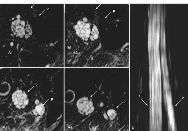
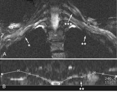
Areas of nerve irritation can be confirmed by comparing the appearance of serial nerve cross sections in the nerve-perpendicular views with those seen in the nerve-parallel views. In nerve-perpendicular images, the fascicle pattern can generally be observed, and this adds further confidence to a finding of focal nerve hyperintensity noticed in the nerve-parallel views. It will demonstrate expansion of the fascicle compartment at the expense of the interfascicular compartment at areas of focal hyperintensity (Fig. 235-1). The nerve-parallel images provide a linear overview.
Nerve Image Reconstruction, Three-Dimensional Reconstruction, and Partial Volume Averaging
In the brachial plexus, multiplanar reformatting is usually sufficient to generate a series of images that can reliably confirm the existence of a focal change in nerve image intensity. This is aided by positioning the patient in the scanner in a manner that tends to straighten the plexus. When a change in fascicle pattern shows increased intensity in the nerve-perpendicular views that matches a change seen in nerve-parallel views (Fig. 235-1), there can be a very high level of confidence about the clinical reality of nerve edema at the location that appears abnormal in the image.
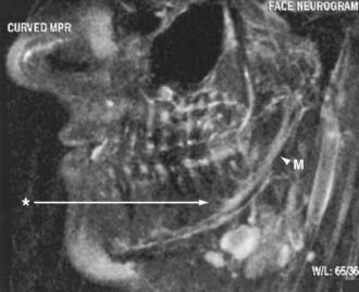
Yet another category of three-dimensional postprocessing is the use of curved reformatting. This step is often capable of producing an image of an extended length of nerve or nerve plexus. The process of curved reformatting can generate a trace of the course of the nerve (Fig. 235-2). This nerve trace is also very useful for interpreting the image because it documents any unusual deviations in the course of a nerve or plexus. However, this method does add some subjectivity to the image analysis process and should not be read without comparison to more objective comparison images such as the original image planes or multiplanar reconstructions.
Conspicuity and Maximum Intensity Projection Images
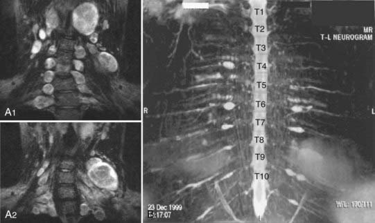
Maximum intensity projections (MIPs) essentially stack up the image slices and have the effect of reassembling the nerves (Fig. 235-3). These MIP images can help in appreciation of the overall course of the nerve and variations in course, caliber, and intensity because they may vary along the length of a nerve.
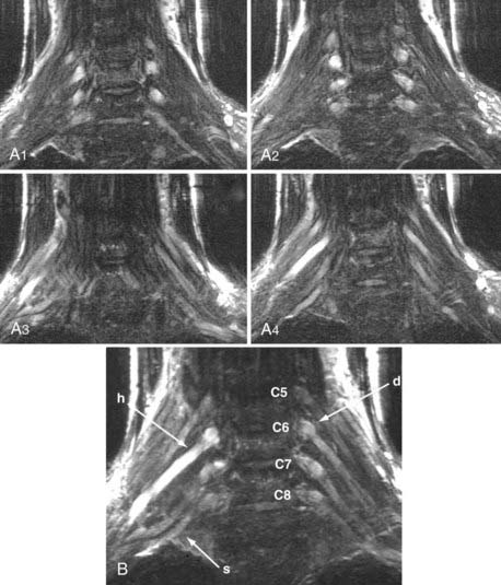
The greatest amount of additional diagnostic information in these analyses occurs in brachial plexus cases.37 Because of the significant incremental amount of clinical information provided by three-dimensional analysis and the susceptibility of most studies to this, these are essential aspects of the diagnostic interpretation process in this group.
Classes of Image Findings
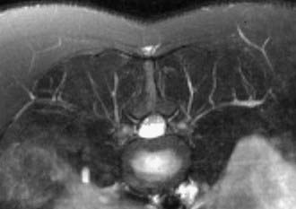
Image findings in MR neurography studies include the presence of regions of nerve hyperintensity or nerve swelling, which result from edema at the fascicular level (see Figs. 235-1 and 235-3). Distortions in the normal course of the nerve, abnormal contours, and alterations in nerve caliber are also readily seen—any of which can be classed by the degree or severity of the abnormality. These findings can indicate entrapment or adhesions, as well as posttraumatic effects.
In patients with hereditary neuropathies, disordered distribution of interfascicular lipid can be detected. The various classes of nerve image findings are most reliable for the larger named nerves greater than 3 mm in diameter, although there is no technical limit on the size of a nerve that can be imaged (Fig. 235-4).
Imaging in the Setting of Nerve Entrapment and Pain
Image Findings in Brachial Plexus Studies
Thoracic Outlet Syndromes
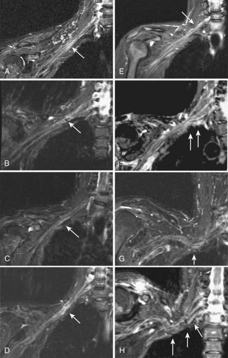
MR neurography has shown promising capability for discriminating among several different types of TOS lesions and in many cases can depict well-delineated and readily treatable specific pathologies.38,39 Such pathologies include distortions of the course of the proximal elements at the scalene triangle (Fig. 235-5A to D), fibrous band entrapments affecting the C8 and T1 spinal nerves and the lower trunk of the brachial plexus (Fig. 235-5F), gross distortions of the midplexus region (Fig. 235-5G and H), irritation at the level of the first rib (Fig. 235-6), and distal plexus irritation.
Brachial Plexus Neuritis
In addition to surgically treatable entrapment, MR neurography is also helpful in identifying patients with complaints attributable to nerve inflammation.40 Such patients often have painless hand atrophy with no associated sensory abnormality. This has sometimes been termed Gilliatt-Sumner hand syndrome. Brachial plexus elements appear bright and swollen but demonstrate no distinct evidence of impingement.
Lumbar Foraminal Pathology
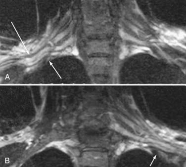
The normal course of the lumbar spinal nerves is a smooth straight line (Fig. 235-7A). In patients with nondiagnostic MRI and myelographic findings, MR neurography can demonstrate distortions of the course of the exiting nerve in the distal foramen (Fig. 235-8A; also see Fig. 235-7B).
Even when myelography is capable of demonstrating that a nerve root is cut off, an MR neurogram can provide considerable additional information. The full length of the foraminal impingement requiring treatment can easily be appreciated on a neurographic image. In addition, the ability of MR neurography to demonstrate hyperintensity in the lumbar root adjacent to the impingement helps confirm the clinical significance of the impingement (Fig. 235-8A). MR neurography is also particularly helpful for imaging foraminal spinal disease in the presence of scoliosis because the three-dimensional aspects of the imaging tend to resolve some of the ambiguities arising from the spatial complexity that may otherwise make diagnosis very challenging.
Magnetic Resonance Neurography in the Pelvis
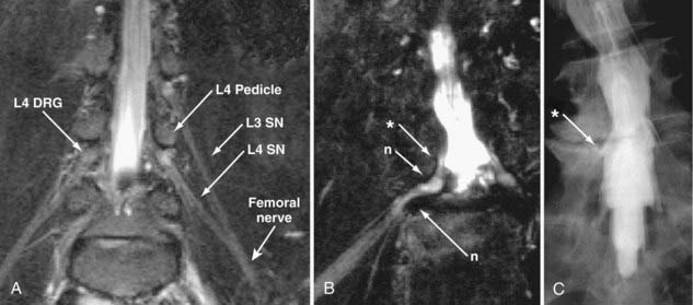
The use of MR neurography has had a significant impact on diagnosis in the pelvis.11,15,16,41,42 Although sciatic pathologies have been an important part of the advance, the ability of MR neurography to track other nerve elements in the pelvis such as the ilioinguinal nerve, pudendal nerve, and lateral femoral cutaneous nerve has gone a long way to resolving what had been a troublesome black box. Imaging of the complete course of the L4 spinal nerve as it progresses into the femoral nerve has made it possible to search for abnormalities along the intra-abdominal and intrapelvic course that previously were almost impossible to diagnose.
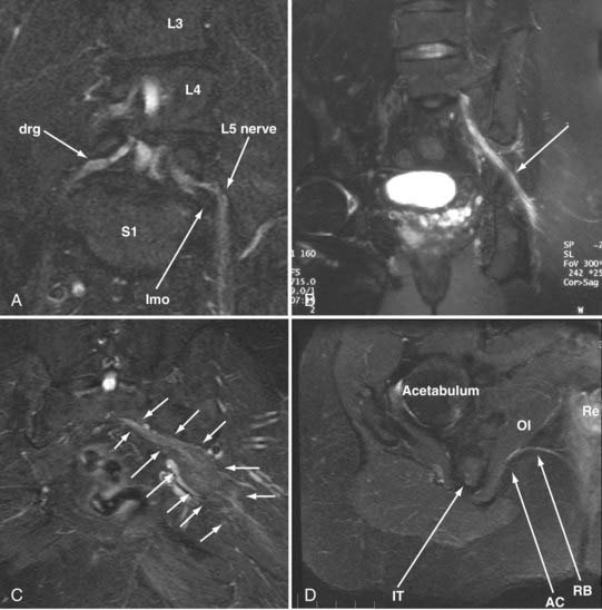
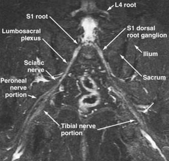
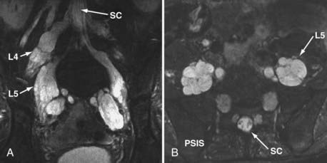
A single imaging study can demonstrate the full course of the L5 and S1 spinal nerves and their descendants in the lumbosacral plexus and proximal sciatic nerve (Fig. 235-9). It is very reliable for demonstrating the presence of a split nerve/split muscle configuration in the setting of a possible piriformis syndrome. Focal sciatic impingements at the ischial margin (see Fig. 235-8C), at the tendon of the obturator internus, at the distal ischial tunnel on the lateral aspect of the ischial tuberosity, and at various locations in the thigh are readily distinguished.
Reliable identification of anatomic variants of the sciatic nerve now plays a critical role in improving the safety of surgery for the release of pelvic sciatic nerve entrapment. Isolated section of a single piriformis segment in patients with a split nerve passing through a split muscle can cause severe nerve compromise from some types of piriformis surgery if this condition is not detected in advance (Fig. 235-9).
Identification of the presence or absence of pudendal nerve irritation in the Alcock canal along the medial aspect of the obturator internus muscle or at the rectal branch of the pudendal nerve proximal to its entrance to the Alcock canal (see Fig. 235-8D) has also been quite useful clinically.16
Distal Entrapments
Identification of distal entrapment of cranial nerves, including the inferior alveolar nerve in the jaw (Fig. 235-10) and the glossopharyngeal nerve as it descends in the upper part of the neck, is also very effective with neurographic imaging.
Nerve Adhesions
An interesting aspect of image-based diagnosis of focal neuropathies is that it has been capable of further elucidating the role of adhesive entrapment and in some cases distinguishing it from compressive entrapment. MR neurography has been particularly helpful in demonstrating the degree to which nerves move across some joints. In Figure 229-5, two images of the median nerve at the carpal tunnel reveal very different positions of the nerve within the tunnel. However, both images are from the same individual and were obtained at the same location in the wrist—they differ only in that one is in a position of flexion and one in extension of the wrist. Imaging of a series of patients with clinically and electrodiagnostically confirmed EMG revealed that although most had compressive lesions, some demonstrated only nerve adhesion with loss of normal mobility of the nerve on flexion and extension of the wrist.
Clinically, this demonstration is of potentially greater importance because in many cases it is possible to demonstrate with imaging that a nerve is not gliding normally across a joint. Restriction of movement of a nerve can cause repeated trauma to the nerve, as well as symptoms of pain exacerbated by extremes of motion or by assuming particular postures or limb positions. When this finding has been documented preoperatively, it becomes possible to plan on taking special measures to reduce the risk for recurrent scar formation postoperatively.43
Reflex Sympathetic Dystrophy
There is no typical image signature associated with complex regional pain syndromes or reflex sympathic dystrophy (RSD). However, it is often the case that idiopathic distortions of the course or contour of a nerve can be identified in patients with RSD. In some patients, the typical history of trauma associated with delayed onset of RSD symptoms may indicate a surgically treatable cause of the pain syndrome (see Fig. 235-8B).
Nerve Trauma
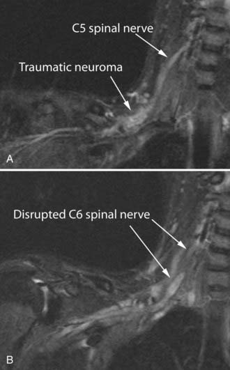
Management of severe nerve trauma has traditionally been complicated by the difficulty of distinguishing between situations in which a nerve will recover with the passage of time and those in which a nerve graft or other sort of surgical treatment would be appropriate. The problem arises because recovery after axonotmesis may require several months but there are few reliable means of distinguishing this situation from neurotmesis, in which no recovery can be expected without surgical intervention. MR neurography can be fairly efficient in establishing the existence of significant nerve injury,44 as well as in demonstrating continuity in a nerve (Fig. 235-12). At present, there still exists a limitation in that hemorrhage immediately after trauma may obscure some details of the nerve image in the first few days after an injury. In the future it is likely that enhancements in MR neurographic pulse sequences will help resolve this problem.
There is still no completely reliable means of confirming true nerve root avulsion by imaging.45 An MR neurographic study includes an effective MR myelogram (Fig. 235-12A) and can therefore demonstrate any meningoceles that may be associated with nerve root avulsions. The procedure is less invasive than CT myelography and provides information of similar quality.
Obstetric Brachial Plexus Injury
A particularly complex situation arises in the management of obstetric brachial plexus injuries. Imaging of infants is difficult, and the need for sedation entails significant additional risks. However, it has proved possible to identify growing terminal neuromas in some locations and to demonstrate continuity of nerves at other sites. As computer techniques for “postprocessing” of images have progressed, it has become possible to generate fairly detailed image representations of complex brachial plexus injuries in children younger than 4 months.27
Follow-up of Nerve-Grafting Procedures
After nerve grafting or after primary early repair of a nerve laceration, several months must elapse before it becomes clear whether the graft has been successful. MR neurography has proved helpful for evaluation of a nerve suture repair site when recovery did not ensue.22 In this case, demonstration of a neuroma at the repair site led to a plan to re-explore and revise the suture repair.
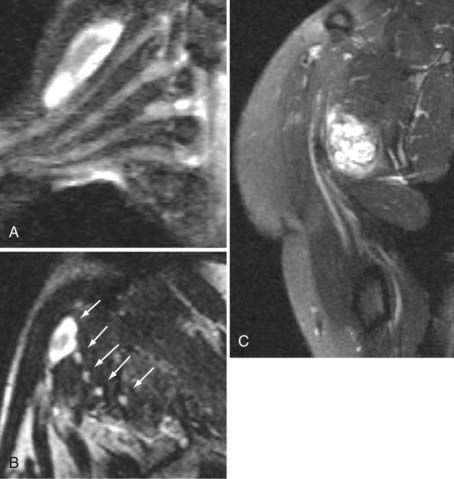
Nerve Tumors
MR neurography permits a directed examination for nerve tumors that has greater sensitivity than other MR methods because of its reliability in showing that a given mass is actually inside a nerve or in direct continuity with it. In any body region the nerves can readily be evaluated for tumors, the symptoms of which are often mistaken for sciatica because of routine spinal pathology. In some cases, the level of detail also allows distinguishing among types of tumors, such as the reported capability of distinguishing perineurioma from schwannoma,46 as well as for identifying very small tumors that just slightly expand the caliber of a nerve.
In addition to the potential for diagnosing a nerve tumor, MR neurography can be extremely helpful in surgical planning for the treatment of these lesions.47 In the setting of a brachial plexus lesion it is possible to definitively distinguish which elements of the plexus are involved in the lesion (Fig. 235-13). It is also often possible to identify the relationship of the main nerve trunk to the mass of the tumor and thus plan the safest possible surgical approach.
Imaging may play a role in the initial diagnosis of neurofibromatosis and is also helpful in tracking and analysis of advanced stages of the disease (Fig. 235-14). Other types of tumor-associated neuropathy can frequently be evaluated quite productively by neurography as well.48
Magnetic Resonance Findings in Systemic Neuropathies
An entirely different image effect is seen in chronic inflammatory demyelinating polyradiculoneuropathy. Affected patients have gross dilation of the fascicles themselves (Fig. 235-15). This alteration reflects an apparent increase in low-protein water inside the fascicles. It is somewhat similar to the pattern seen in wallerian degeneration. Although some onion bulb formations are seen in sural nerve biopsy specimens from these patients, there are perivascular mononuclear cells and notable edema in the endoneurial fluid compartment.49
Diagnosis of Pathologies Affecting Muscle
A variety of types of muscle pathology can be assessed by imaging.50–52 MRI can contribute to diagnosis by providing precise information about the location and distribution of involved muscle tissues, as well as by providing qualitative information about several types of abnormalities. Abnormal muscle may demonstrate hypertrophy, atrophy, excess fluid—findings causing brightness on T2 imaging—or fatty replacement causing brightness on T1 imaging. The pattern of muscle involvement in these abnormalities, as well as the distribution of these findings within individual muscles and muscle groups, can provide valuable diagnostic information.
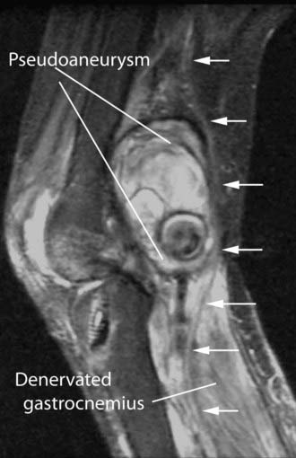
Imaging of Denervated Muscle
In a variety of situations, MRI can be a useful adjunct to electrodiagnostic studies for the evaluation of muscle denervation. Denervated muscle becomes hyperintense when imaged with a standard T2-based MR neurography protocol. When this phenomenon is present, it greatly simplifies the task of identifying individual muscles involved in a selective focal or distal injury (Fig. 235-16).
The development of signal alterations in muscle after denervation was first reported by Shabas and associates53 and by Polak and colleagues.54 It is now known that abnormal muscle appearance may be detected as early as 4 days after an axonotmetic or neurotmetic injury. The signal abnormalities become progressively more intense as months pass and reach a maximum about 4 months from the date of injury. In the 1- to 2-year range, the quality of the abnormality changes but it will continue to persist unless the nerve regrows or is restored through grafting.
The initial change is increased intensity on T2-weighted imaging. This has been observed by using an “inversion recovery” pulse sequence called STIR (short tau inversion recovery), as well as other T2-weighted, fat-suppressed sequences used for neurography. Animal work has shown how the appearance of increased signal occurs.55 There is no increase in water content of the muscle; however, the use of radiolabeled tracer compounds allowed the authors to establish that extracellular fluid volume was expanded at the expense of intracellular fluid. This shift was apparently associated with atrophy of the muscle cells.
A larger detailed human study by Fleckenstein and coworkers established that the onset of imaging changes is variable from patient to patient and that there is variability in the effect even among muscles in the distribution of a single damaged nerve.51 In the 1- to 2-year range, the quality of the abnormality changes as the muscles undergo substitution with fat. This additional change may correlate with the development of nonreceptivity to regrowing nerve fibers, which is known to take place at a similar interval after denervation; however, this concept has not yet been firmly established. Fleckenstein and associates also point out that muscle edema from trauma, as well as several other confounding sources of image abnormalities, must be kept in mind when considering this type of data.
Additional information about the clinical utility of muscle imaging was presented in a report on imaging of 32 patients by West and coauthors.56 They documented a similar range of alterations in image appearance in a case study format. These authors advocated the use of MRI to assess muscle denervation in patients who do not tolerate electrodiagnostic tests well, such as small children, in patients needing serial testing, and in patients in whom a complete view of the detailed pattern of innervation is required for surgical planning.
Myopathic and Neuropathic Effects on Muscle Image Patterns
In a number of myopathies and neuropathies, two aspects of muscle degeneration can be appreciated on imaging. There may be an increase in the T2 relaxation time of resting muscle because of effective edema in the muscle fibers.57–59 In addition, characteristic patterns of fatty replacement or degenerative change have been described for several conditions. These changes can readily be appreciated on fat-suppressed T1-weighted images.60–62 Changes in the T2 or T1 image parameters of muscle and the distribution of these changes have been reported for amyotrophic lateral sclerosis as well.63 Painful myopathies in diabetics can be evaluated with MRI to learn whether muscle infarction is playing a role as opposed to a more strictly neuropathic source of the pain.64
Aagaard BD, Maravilla KR, Kliot M. Magnetic resonance neurography: magnetic resonance imaging of peripheral nerves. Neuroimaging Clin N Am. 2001;11:viii.
Dailey AT, Tsuruda JS, Filler AG, et al. Magnetic resonance neurography of peripheral nerve degeneration and regeneration. Lancet. 1997;350:1221.
Filler; Filler AG. MR Neurography and diffusion tensor imaging: origins, history & clinical impact of the first 50,000 cases with an assessment of efficacy and utility in a prospective 5,000 patient study group. Neurosurgery. (in press).
Filler AG. Piriformis and related entrapment syndromes: diagnosis and management. Neurosurg Clin N Am. 2008;19:609.
Filler AG. Diagnosis and management of pudendal nerve entrapment syndromes: impact of MR neurography and open MR-guided injections. Neurosurg Q. 2008;18:1.
Filler AG. MR Neurography and brachial plexus neurolysis in the management of thoracic outlet syndromes. In: Yao JST, Pearce WH, editors. Advances in Vascular Surgery. Chicago: Precept Press; 2002:499.
Filler AG, Bell BA. Axonal transport, imaging, and the diagnosis of nerve compression. Br J Neurosurg. 1992;6:293.
Filler AG, Haynes J, Jordan SE, et al. Sciatica of nondisc origin and piriformis syndrome: diagnosis by magnetic resonance neurography and interventional magnetic resonance imaging with outcome study of resulting treatment. J Neurosurg Spine. 2005;2:99.
Filler AG, Howe FA, Hayes CE, et al. Magnetic resonance neurography. Lancet. 1993;341:659.
Filler AG, Kliot M, Howe FA, et al. Application of magnetic resonance neurography in the evaluation of patients with peripheral nerve pathology. J Neurosurg. 1996;85:299.
Filler AG, Maravilla KR, Tsuruda JS. MR neurography and muscle MR imaging for image diagnosis of disorders affecting the peripheral nerves and musculature. Neurol Clin. 2004;22:643.
Grant GA, Britz GW, Goodkin R, et al. The utility of magnetic resonance imaging in evaluating peripheral nerve disorders. Muscle Nerve. 2002;25:314.
Grant GA, Goodkin R, Maravilla KR, et al. MR neurography: diagnostic utility in the surgical treatment of peripheral nerve disorders. Neuroimaging Clin N Am. 2004;14:115.
Howe FA, Filler AG, Bell BA, et al. Magnetic resonance neurography. Magn Reson Med. 1992;28:328.
Jarvik JG, Comstock BA, Heagerty PJ, et al. Magnetic resonance imaging compared with electrodiagnostic studies in patients with suspected carpal tunnel syndrome: predicting symptoms, function, and surgical benefit at 1 year. J Neurosurg. 2008;108:541.
Jarvik JG, Yuen E, Haynor DR, et al. MR nerve imaging in a prospective cohort of patients with suspected carpal tunnel syndrome. Neurology. 2002;58:1597.
Khalil C, Hancart C, Le Thuc V, et al. Diffusion tensor imaging and tractography of the median nerve in carpal tunnel syndrome: preliminary results. Eur Radiol. 2008;18:2283.
Kuntz C, Blake L, Britz G, et al. Magnetic resonance neurography of peripheral nerve lesions in the lower extremity. Neurosurgery. 1996;39:750.
Lewis AM, Layzer R, Engstrom JW, et al. Magnetic resonance neurography in extraspinal sciatica. Arch Neurol. 2006;63:1469.
Myers RR, Rydevik BL, Heckman HM, et al. Proximodistal gradient in endoneurial fluid pressure. Exp Neurol. 1988;102:368.
Raphael DT, McIntee D, Tsuruda JS, et al. Frontal slab composite magnetic resonance neurography of the brachial plexus: implications for infraclavicular block approaches. Anesthesiology. 2005;103:1218.
Singh T, Kliot M. Imaging of peripheral nerve tumors. Neurosurg Focus. 2007;22(6):E6.
Smith AB, Gupta N, Strober J, et al. Magnetic resonance neurography in children with birth-related brachial plexus injury. Pediatr Radiol. 2008;38:159.
West GA, Haynor DR, Goodkin R, et al. Magnetic resonance imaging signal changes in denervated muscles after peripheral nerve injury. Neurosurgery. 1994;35:1077.
Yoshikawa T, Hayashi N, Yamamoto S, et al. Brachial plexus injury: clinical manifestations, conventional imaging findings, and the latest imaging techniques. Radiographics. 2006;26(suppl 1):S133.
1 Howe FA, Filler AG, Bell BA, et al. Magnetic resonance neurography. Magn Reson Med. 1992;28:328.
2 Howe FA, Filler AG, Bell BA, et al. Magnetic resonance neurography: optimizing imaging techniques for peripheral nerve identification. Paper presented at the 11th Annual Meeting of the Society for Magnetic Resonance in Medicine. Berlin; 1991:1701.
3 Filler AG, Bell BA. Axonal transport, imaging, and the diagnosis of nerve compression. Br J Neurosurg. 1992;6:293.
4 Filler AG, Tsuruda JS, Richards TL, et al. Images, Apparatus, Algorithms and Methods. GB 9216383: UK Patent Office, 1992.
5 Richards TL, Heide AC, Tsuruda JS, et al. Vector analysis of diffusion images in experimental allergic encephalomyelitis. Paper presented at a meeting of the Society for Magnetic Resonance in Medicine. Berlin; 1992:412.
6 Kline DG, Hudson AR, Zager E. Selection and preoperative work-up for peripheral nerve surgery. Clin Neurosurg. 1992;39:8.
7 Filler AG, Winn HR, Howe FA, et al. Axonal transport of superparamagnetic metal oxide particles: potential for magnetic resonance assessments of axoplasmic flow in clinical neuroscience. Paper presented at the 10th Annual Meeting of the Society for Magnetic Resonance in Medicine. San Francisco; 1991:985.
8 Filler AG, Howe FA, Hayes CE, et al. Magnetic resonance neurography. Lancet. 1993;341:659.
9 Filler AG, Tsuruda JS, Richards TL, et al. Image Neurography and Diffusion Anisotropy Imaging. US 5,560,360: Unites States Patent Office, 1993.
10 Heide AC, Richards TL, Alvord EC, et al. Diffusion imaging of experimental allergic encephalomyelitis. Magn Reson Med. 1993;29:478.
11 Filler AG, Haynes J, Jordan SE, et al. Sciatica of nondisc origin and piriformis syndrome: diagnosis by magnetic resonance neurography and interventional magnetic resonance imaging with outcome study of resulting treatment. J Neurosurg Spine. 2005;2:99.
12 Jarvik JG, Yuen E, Haynor DR, et al. MR nerve imaging in a prospective cohort of patients with suspected carpal tunnel syndrome. Neurology. 2002;58:1597.
13 Jarvik JG, Comstock BA, Heagerty PJ, et al. Magnetic resonance imaging compared with electrodiagnostic studies in patients with suspected carpal tunnel syndrome: predicting symptoms, function, and surgical benefit at 1 year. J Neurosurg. 2008;108:541.
14 Atlas SW. Magnetic Resonance Imaging of the Brain and Spine, 3rd ed. Philadelphia: Lippincott Williams & Wilkins; 2002.
15 Filler AG. Piriformis and related entrapment syndromes: diagnosis and management. Neurosurg Clin N Am. 2008;19:609.
16 Filler AG. Diagnosis and management of pudendal nerve entrapment syndromes: impact of MR neurography and open MR-guided injections. Neurosurg Q. 2008;18:1.
17 Filler AG. MR neurography and diffusion tensor imaging: origins, history & clinical Impact of the first 50,000 cases with an assessment of efficacy and utility in a prospective 5,000 patient study group. Neurosurgery. (in press).
18 Aagaard BD, Maravilla KR, Kliot M. MR neurography. MR imaging of peripheral nerves. Magn Reson Imaging Clin N Am. 1998;6:179.
19 Aagaard BD, Maravilla KR, Kliot M. Magnetic resonance neurography: magnetic resonance imaging of peripheral nerves. Neuroimaging Clin N Am. 2001;11:viii.
20 Kuntz Ct, Blake L, Britz G, et al. Magnetic resonance neurography of peripheral nerve lesions in the lower extremity. Neurosurgery. 1996;39:750.
21 Filler AG, Kliot M, Howe FA, et al. Application of magnetic resonance neurography in the evaluation of patients with peripheral nerve pathology. J Neurosurg. 1996;85:299.
22 Dailey AT, Tsuruda JS, Filler AG, et al. Magnetic resonance neurography of peripheral nerve degeneration and regeneration. Lancet. 1997;350:1221.
23 Bowen BC, Pattany PM, Saraf-Lavi E, et al. The brachial plexus: normal anatomy, pathology, and MR imaging. Neuroimaging Clin N Am. 2004;14:59.
24 Grant GA, Britz GW, Goodkin R, et al. The utility of magnetic resonance imaging in evaluating peripheral nerve disorders. Muscle Nerve. 2002;25:314.
25 Grant GA, Goodkin R, Maravilla KR, et al. MR neurography: diagnostic utility in the surgical treatment of peripheral nerve disorders. Neuroimaging Clin N Am. 2004;14:115.
26 Filler AG, Maravilla KR, Tsuruda JS. MR neurography and muscle MR imaging for image diagnosis of disorders affecting the peripheral nerves and musculature. Neurol Clin. 2004;22:643.
27 Smith AB, Gupta N, Strober J, et al. Magnetic resonance neurography in children with birth-related brachial plexus injury. Pediatr Radiol. 2008;38:159.
28 Khalil C, Hancart C, Le Thuc V, et al. Diffusion tensor imaging and tractography of the median nerve in carpal tunnel syndrome: preliminary results. Eur Radiol. 2008;18:2283.
29 Tsuchiya K, Imai M, Tateishi H, et al. Neurography of the spinal nerve roots by diffusion tensor scanning applying motion-probing gradients in six directions. Magn Reson Med Sci. 2007;6:1.
30 Viallon M, Vargas MI, Jlassi H, et al. High-resolution and functional magnetic resonance imaging of the brachial plexus using an isotropic 3D T2 STIR (short term inversion recovery) SPACE sequence and diffusion tensor imaging. Eur Radiol. 2008;18:1018.
31 Moseley ME, Kucharczyk J, Asgari HS, et al. Anisotropy in diffusion-weighted MRI. Magn Reson Med. 1991;19:321.
32 Mizisin AP, Kalichman MW, Myers RR, et al. Role of the blood-nerve barrier in experimental nerve edema. Toxicol Pathol. 1990;18:170.
33 Poduslo JF, Low PA, Nickander KK, et al. Mammalian endoneurial fluid: collection and protein analysis from normal and crushed nerves. Brain Res. 1985;332:91.
34 Myers RR, Rydevik BL, Heckman HM, et al. Proximodistal gradient in endoneurial fluid pressure. Exp Neurol. 1988;102:368.
35 Chappell KE, Robson MD, Stonebridge-Foster A, et al. Magic angle effects in MR neurography. AJNR Am J Neuroradiol. 2004;25:431.
36 Hayes CE, Tsuruda JS, Mathis CM, et al. Brachial plexus: MR imaging with a dedicated phased array of surface coils. Radiology. 1997;203:286.
37 Raphael DT, McIntee D, Tsuruda JS, et al. Frontal slab composite magnetic resonance neurography of the brachial plexus: implications for infraclavicular block approaches. Anesthesiology. 2005;103:1218.
38 Filler AG. MR Neurography and brachial plexus neurolysis in the management of thoracic outlet syndromes. In: Yao JST, Pearce WH, editors. Advances in Vascular Surgery. Chicago: Precept Press; 2002:499.
39 Filler AG, Johnson JP, Machleder H, et al. Neurographic findings in diagnosis of thoracic outlet syndrome [abstract]. In: Proceedings of the Congress of Neurological Surgeons Annual Meeting, New Orleans, LA. Neurosurgery. 1997;41:724.
40 Zhou L, Yousem DM, Chaudhry V. Role of magnetic resonance neurography in brachial plexus lesions. Muscle Nerve. 2004;30:305.
41 Moore KR, Tsuruda JS, Dailey AT. The value of MR neurography for evaluating extraspinal neuropathic leg pain: a pictorial essay. AJNR Am J Neuroradiol. 2001;22:786.
42 Lewis AM, Layzer R, Engstrom JW, et al. Magnetic resonance neurography in extraspinal sciatica. Arch Neurol. 2006;63:1469.
43 McCall TD, Grant GA, Britz GW, et al. Treatment of recurrent peripheral nerve entrapment problems: role of scar formation and its possible treatment. Neurosurg Clin N Am. 2001;12:329.
44 Cornwall R, Radomisli TE. Nerve injury in traumatic dislocation of the hip. Clin Orthop Relat Res. 2000;377:84.
45 Yoshikawa T, Hayashi N, Yamamoto S, et al. Brachial plexus injury: clinical manifestations, conventional imaging findings, and the latest imaging techniques. Radiographics. 2006;26(suppl 1):S133.
46 Heilbrun ME, Tsuruda JS, Townsend JJ, et al. Intraneural perineurioma of the common peroneal nerve. Case report and review of the literature. J Neurosurg. 2001;94:811.
47 Singh T, Kliot M. Imaging of peripheral nerve tumors. Neurosurg Focus. 2007;22(6):E6.
48 Moore KR, Blumenthal DT, Smith AG, et al. Neurolymphomatosis of the lumbar plexus: high-resolution MR neurography findings. Neurology. 2001;57:740.
49 Dyck PJ, Prineas J, Pollard J. Chronic inflammatory demyelinating polyradiculopathy. In: Dyck PJ, Thomas P, editors. Peripheral Neuropathy. Philadelphia: WB Saunders; 1993:1498.
50 Bosboom EM, Bouten CV, Oomens CW, et al. Quantifying pressure sore–related muscle damage using high-resolution MRI. J Appl Physiol. 2003;95:2235.
51 Fleckenstein JL, Watumull D, Conner KE, et al. Denervated human skeletal muscle: MR imaging evaluation. Radiology. 1993;187:213.
52 Ozsarlak O, Schepens E, Parizel PM, et al. Hereditary neuromuscular diseases. Eur J Radiol. 2001;40:184.
53 Shabas D, Gerard G, Rossi D. Magnetic resonance imaging examination of denervated muscle. Comput Radiol. 1987;11:9.
54 Polak JF, Jolesz FA, Adams DF. Magnetic resonance imaging of skeletal muscle. Prolongation of T1 and T2 subsequent to denervation. Invest Radiol. 1988;23:365.
55 Polak JF, Jolesz FA, Adams DF. NMR of skeletal muscle. Differences in relaxation parameters related to extracellular/intracellular fluid spaces. Invest Radiol. 1988;23:107.
56 West GA, Haynor DR, Goodkin R, et al. Magnetic resonance imaging signal changes in denervated muscles after peripheral nerve injury. Neurosurgery. 1994;35:1077.
57 Meola G, Sansone V, Rotondo G, et al. Computerized tomography and magnetic resonance muscle imaging in Miyoshi’s myopathy. Muscle Nerve. 1996;19:1476.
58 Reimers CD, Schedel H, Fleckenstein JL, et al. Magnetic resonance imaging of skeletal muscles in idiopathic inflammatory myopathies of adults. J Neurol. 1994;241:306.
59 Jonas D, Conrad B, Von Einsiedel HG, et al. Correlation between quantitative EMG and muscle MRI in patients with axonal neuropathy. Muscle Nerve. 2000;23:1265.
60 Mercuri E, Cini C, Counsell S, et al. Muscle MRI findings in a three-generation family affected by Bethlem myopathy. Eur J Paediatr Neurol. 2002;6:309.
61 Mercuri E, Pichiecchio A, Counsell S, et al. A short protocol for muscle MRI in children with muscular dystrophies. Eur J Paediatr Neurol. 2002;6:305.
62 Ikeda K, Kinoshita M, Iwasaki Y, et al. Unusual fatty infiltration of the soleus muscle in a patient with congenital nemaline myopathy: fat-suppression muscle MRI. Intern Med. 2002;41:237.
63 Bryan WW, Reisch JS, McDonald G, et al. Magnetic resonance imaging of muscle in amyotrophic lateral sclerosis. Neurology. 1998;51:110.
64 Van Slyke MA, Ostrov BE. MRI evaluation of diabetic muscle infarction. Magn Reson Imaging. 1995;13:325.