Introduction

For generations, investigators have pursued the heritable contribution to cancer. Seminal studies in families with several members affected with breast cancer, colorectal cancer, melanoma, or a constellation of cancers (e.g., Li-Fraumeni syndrome) provided evidence for rare mutations with strong effects.¹ Family-based and twin studies indicate an excess familial cancer aggregation for nearly all types of cancers, although the estimates vary greatly across cancer types. These observations suggested that it would be possible to map cancer genes and thus estimate the genetic contribution to each molecular type of cancer, even in unrelated populations. Until the past decade, progress has been slow. However, the pace at which new genetic regions harboring cancer susceptibility alleles have been discovered has accelerated substantially as a result of three converging factors: first, a high-quality draft sequence of the human genome was produced^2,3; second, its subsequent annotation has resulted in the appreciation of a wide spectrum of variation across the genome⁴; and third, the development of technical platforms that enable interrogation of genetic variation across the genome has changed both the economics and speed with which genetic studies can be performed. The scope of studies has thus changed dramatically, expanding from family-based studies to larger population-based studies of unrelated individuals. These studies have been fueled by the precipitous drop in price for interrogating single nucleotide polymorphisms (SNPs), the most common type of variant in the genome, or massive parallel sequence analysis of entire or partial genomes. To keep pace with the new streams of large data sets, investigators have forged new collaborations and developed computational tools for analyzing larger data sets in search of new cancer susceptibility alleles.

Cancer susceptibility alleles have been discovered with the use of a variety of approaches, yielding a range of inherited genetic variants, from rare mutations with strong effects (e.g., highly penetrant) to common genetic polymorphisms, each of which confers a small risk for cancer.¹ Susceptibility alleles can increase a person’s risk of developing cancer either within families or across populations. It is notable that not all susceptibility alleles have equal estimated effects. Consequently, the observed spectrum of established susceptibility alleles reflects an inverse relationship between the effect size and the frequency of the genetic variation (Fig. 22-1).^5,6 Highly penetrant mutations are rare and have a strong predictive value for developing one or more cancers. These highly penetrant mutations are generally discovered in family studies using linkage analysis and, more recently, next-generation sequencing analysis in and across pedigrees in which several family members are affected with the same or a constellation of cancers. More frequent susceptibility alleles have smaller effect sizes and are discovered using association studies in which the genomes of a set of affected cases are compared with that of unaffected control subjects.⁷

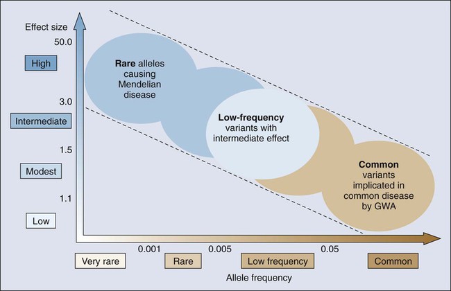
Genetic mapping of cancer susceptibility genes can identify regions of the genome harboring genes that play a role in cancer susceptibility but also nongenic regions that can regulate genes and pathways of interacting genes. Although the direct public health impact associated with conclusively establishing a specific cancer susceptibility allele may not be immediately apparent, its contribution to understanding tumor development and metastasis is invaluable, expanding possible pathways and putative targets for intervention downstream.⁸ Moreover, the possible clinical value of known susceptibility alleles will continue to increase as more comprehensive maps of susceptibility alleles emerge for specific cancers. Thus far, there are more distinct susceptibility alleles per cancer than there are susceptibility alleles that contribute to the risk for multiple cancers. To define the genetic architecture (Fig. 22-1), namely, the constellation of susceptibility alleles that contributes to a specific cancer, further efforts are required to define comprehensive sets of variants, which in turn should emerge as vital tools in both public health and individual (known as precision medicine) assessments of cancer risk.⁹

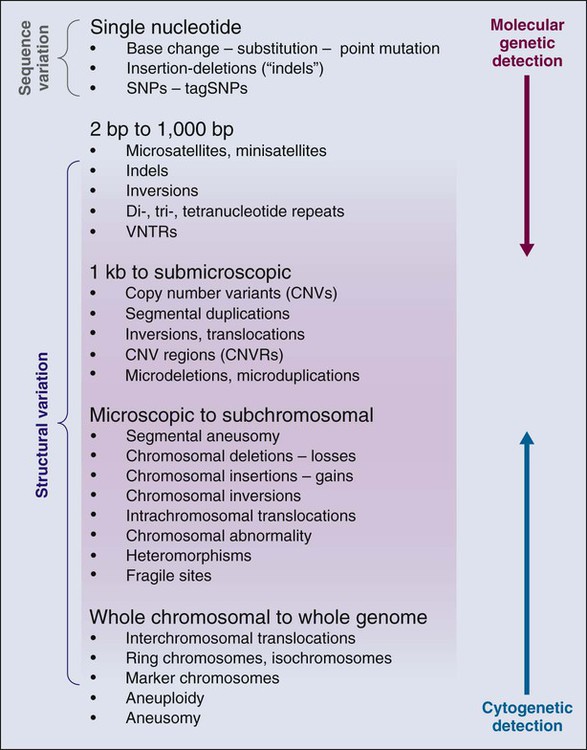
The annotation of genetic variation in the genome has provided important clues to elucidation of the genetic history of distinct populations, possible interactions between environmental or pathogen challenges, and the heterogeneous distribution of human cancers. The differences in the spectrum of allele frequencies and the types of genetic variation, from SNPs to large copy number variants, have become indispensable tools for geneticists to map diseases (Fig. 22-2).^4,10–12 The basic principle has been to observe distinct patterns of genetic variation between affected and unaffected individuals, whether in families or population studies.

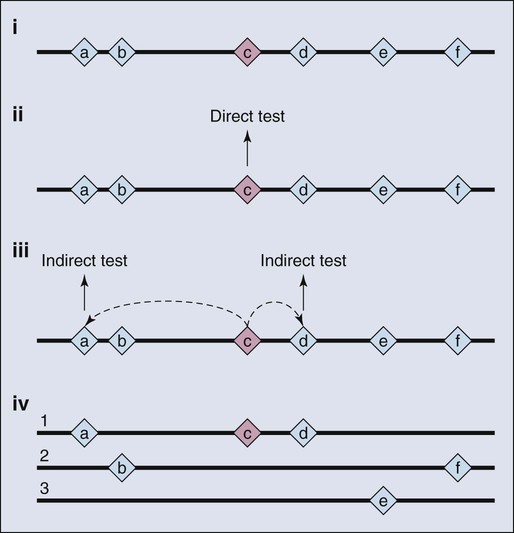
As a consequence of the enormous scope of human genetic variation, the search for susceptibility alleles has broadened and for most study designs has focused on conclusively discovering “markers” that highlight the region of the genome where a disease susceptibility alleles resides.¹³ Sets of markers to be tested are drawn from dense maps of human genetic variation that are publicly available. The approach is not predicated on testing the actual casual variant, at least not initially, but instead identifying one or more surrogates that are highly correlated with the variant actually underlying the susceptibility allele. Although embracing this “indirect” approach has had great value (Fig. 22-3), it comes at a price, namely, additional steps to sort through the correlated variants and then conduct the functional studies needed to illuminate the underpinnings of the susceptibility allele.¹³ In other words, further work is required to characterize the mutations directly responsible for contribution to disease susceptibility (also known as causal mutations).¹⁴

Until it was possible to envision a whole genome sequence, genetics had created and modified maps of relative coordinates based on incomplete constructs. Sets of markers can be thought of as molecular street signs, which allowed one to knowingly navigate his or her way up or down a chromosome. Early on, “genetic maps” provided a stable reference for mapping highly penetrant mutations, primarily in families.¹⁵ These maps were based on empirical evidence of recombination hot spots. The long-standing value of functional elements, herein recombination frequencies, served adequately for the mapping of disease and traits before the draft sequences of genomes began to appear. The emergence of a physical map (currently tractable for more than 92% of the genome) has accelerated the mapping of traits and diseases because the field has closed in on absolute coordinates for the genome. That is, we generally know the nucleotide location of a given marker or gene in millions of base pairs from the end or terminus of the chromosome. Investigators still use the principles uncovered in studying genetic maps to pinpoint alleles on the physical map.

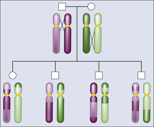
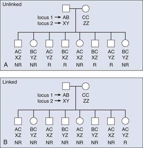
The principles of meiotic recombination are key to understanding the relationship between genetic loci, here defined as genetic variants that map to unique coordinates on the physical map. The correlation between genetic markers is fundamental to both association and linkage analysis. In meiosis, the cell division leading to gamete formation and homologous chromosomes are paired. Each chromosome consists of two identical strands (chromatids), with each chromosome pairing composed of four strands. Homologous chromosomes separate from each other during the process of meiosis except at one or two zones of contact in a process that leads to genetic recombination (Fig. 22-4). Mendel’s second law, independent assortment, states that alleles of genes at unlinked loci segregate or assort independently of one another. Deviations from independent assortment occur when genes are located close to one another, in which case alleles assort together more than 50% of the time. In this scenario, the associated loci are “linked.” Distributed throughout the genome are recombination hot spots, which “divide” the genome. These hot spots can vary by population genetic history, providing an opportunity to compare groups and use the differences to pinpoint possible susceptibility alleles, especially if substantive differences exist between populations with respect to cancer incidence.

Consequently, if two loci are located on different chromosomes or far apart on the same chromosome, their alleles will assort randomly, transmitting to the same gamete 50% of the time. Such loci are “unlinked.” For a chromosomal segment, the probability of a genetic recombination event occurring between a pair of markers is proportional to the distance between them. This probability is expressed as a recombination frequency (q), where θ = number of recombinant offspring/number of total offspring. The closer a marker and disease gene were located on a chromosome, the lower the probability they would be dissociated during recombination events. Conversely, the farther apart they were, the higher the probability they would appear “unlinked” in multiple generations of a family. The recombination frequency values range from 0 for markers that are so closely linked that crossover events essentially never occur to 0.5 for genes that assort randomly—for instance, those on different chromosomes or chromosome arms. Within small intervals, when the probability of multiple crossovers is negligible the relationship between the recombination fraction (θ) and the distance between two genes (x), is simply x = θ.¹⁶ After a mathematical adjustment for the small possibility of double recombinants, recombination fractions are expressed in units called centimorgans (cMs).¹⁷ One percent recombination (θ = 0.01) is equal to 1 cM for the genetic map, which, in the human genome, corresponds to about one million base pairs.

The spectrum of human genetic variation varies by the frequency of polymorphisms, which often is substantial between populations, as well as the length of the variant. The most common sequence variation is the substitution of a single base, known as an SNP, which, by definition, is observed in at least 1% in one or more populations. The minor allele frequency (MAF) refers to the lower allele frequency, and it can vary by population. The number of SNPs increases across the genome as the frequency decreases.¹⁸ A substantially larger fraction of genetic variation exists for single base substitutions below 1%, and many of these are population private, reflecting the population genetics history.¹⁸ The majority of SNPs with an MAF greater than 10% are common to all human populations, but the actual frequencies can vary greatly. Reported SNPs are cataloged in the dbSNP database (http://www.ncbi.nlm.nih.gov/snp), which is an important reference that points to emerging data sets and is useful in interpreting variants identified through DNA sequencing.

A small subset of SNPs are located in exons, of which a fraction change the predicted amino acid. SNPs that can alter the coding sequence are known as nonsynonymous SNPs, whereas those that are silent are termed synonymous. Although great interest has been expressed in coding SNPs, partly because they appear to be more interpretable, very few of the known associations between a disease and a common SNP marker (MAF >10%) are for coding SNPs. On the other hand, rare highly penetrant mutations mainly map to coding changes or preterminal stop codons. Many of the reported disease mutations are cataloged in a public database, the Online Mendelian Inheritance in Man (http://www.ncbi.nlm.nih.gov/sites/entrez?db=OMIM/).

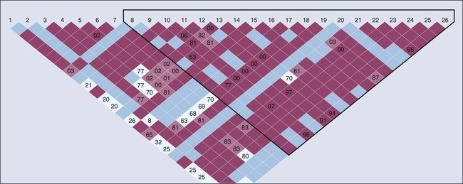
SNPs become fixed in populations over multiple generations and are generally not inherited independent of the adjacent variants. Recombination hot spots can separate sets of highly correlated variants, resulting in “blocks of haplotypes” (Fig. 22-5).¹⁹ These segments of a chromosome, which usually are quite small, are transmitted as a unit from one generation to the next. The correlation between SNPs is an estimate of linkage disequilibrium (LD), which is classically defined as the nonrandom association of alleles at different loci. Individual SNPs that always track together are said to be in strong LD. This correlation can be eroded over time by recombination (exchange of genetic material) during meiosis, and SNPs can be defined as being in weak LD²⁰—that is, a correlation exists, but it is not strong. We measure the degree of LD with use of either D′ or r² coefficients; both give similar information, but the latter are more highly dependent on the MAFs of the adjacent SNPs and are generally more favored by geneticists.

The concept of LD is important because it enables investigators to evaluate sets of SNPs and determine proxies for other, untested SNPs, which is useful for “indirect” mapping. Thus if a group of SNPs are in strong LD and are always inherited together, one can test for the alleles of just one reference SNP and immediately have information regarding which alleles are segregating to a given individual for all the adjacent SNPs. By extension, estimates of LD are useful to construct haplotypes in unrelated subjects. With new reference data sets (e.g., the 1000 Genome Project), it is possible to impute untested variants against the backbone of stable data sets.¹⁸ The computational efficiencies enable estimation of the correlation between sets of markers and the construction of haplotypes.²¹ Still, the most reliable approach is to resolve the phase of haplotypes in multigeneration pedigrees, in which haplotypes can be traced; alternatively, one can infer the relationship of alleles in unrelated subjects with computational tools.²² Phase refers to the parental (and grandparental) chromosome of origin for a set of alleles.²³ This specific information regarding a set of markers in LD can, in turn, be useful for determining where a disease allele originates.

The annotation of the human genome has revealed a wide spectrum of structural variations, which may be either cytologically visible or detected by either microarray chips or actual sequence analysis (Fig. 22-2). For instance, short tandem repeats are a class of polymorphisms in which a small number of base pairs are reiterated, such as “CACACA.” Polymerase chain reaction primers are used to define the physical location of one short tandem repeat from the remaining 50,000 that litter the genome. Also known as microsatellites, they have been effectively used for linkage analysis and forensic investigation. Structural variants of all sizes can include deletions, insertions, and duplications collectively known as copy number variations (CNVs).^12–12 In addition, infrequent inversions and translocations of pieces of DNA are present that vary in size. Some of these inversions and translocations are quite common; for example, chromosome 17 harbors an inversion of 3.5 million base pairs in approximately 20% of the European population.²⁴ CNVs have been shown to influence gene dosage and therefore can contribute to risk for cancer, as demonstrated for a chromosome 1 CNV and the risk for childhood neuroblastoma.²⁵ Accurately determining CNVs from SNP microarrays continues to be a formidable technical challenge, but with new resources and sequencing technologies, termed “next generation sequencing,” it is anticipated that precision will continue to improve, which, in turn, should lead to improved detection of CNVs associated with disease outcomes.

Principles of Linkage Mapping

Many epidemiological studies indicate the presence of a familial contribution, such as the observation that family history of a specific cancer within first-degree relatives is associated with a doubling or more of risk among relatives, particularly in twin registries.26,27 In the case of prostate cancer, for instance, studies of selected hospital-based patient populations, population-based case-control studies, and cohort studies all demonstrate that a family history of disease is correlated with an increase in an individual’s risk. If the affected family members are first-degree relatives (e.g., brothers or fathers and sons), the risk increases from 1.7-fold to 3.7-fold. Younger ages at diagnosis and multiple affected relatives with the disease tend to be associated with even higher relative risk.^28–31 For example, men with three or more first-degree relatives with prostate cancer have an almost elevenfold increased risk of the disease compared with men who have no known family history of the disease.²⁹ For this reason, families ascertained for linkage analysis studies tend to be large, have multiple affected individuals, and feature people who were diagnosed with the disease at a comparatively young age.

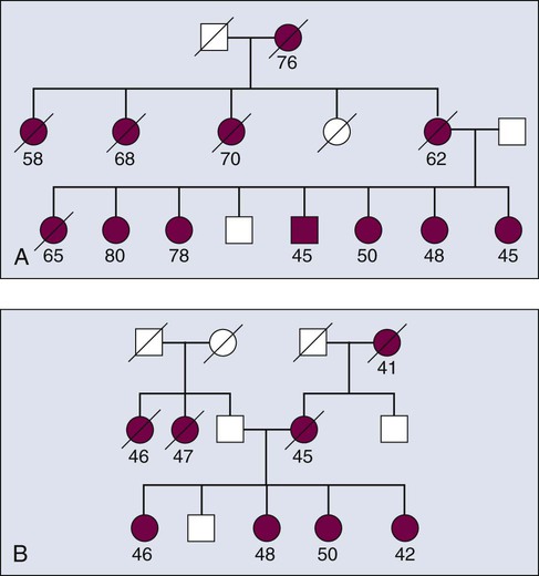
Familial aggregation describes the occurrence of multiple cases of cancer within a family (Fig. 22-6). Clustering of familial cases may be due to shared environment, shared alleles of particular genes, or simply chance if the tumor is very common in the population. In mapping of cancer susceptibility genes for many cancers, particularly for breast and colon cancer, the most promising pedigrees for hereditary cancer are families with three or more first-degree relatives with a given cancer, three successive generations with cancer, or at least two siblings with the same cancer detected at a relatively young age. First-degree relatives are parents, offspring, or siblings.

To identify highly penetrant mutations, success directly correlates with the identification and collection of high-risk or hereditary families. To achieve the numbers needed to improve the power to detect a disease allele, whether using microsatellites, SNP arrays, or next-generation sequencing, large consortium groups are often formed, providing an opportunity to increase power through collection of more families and the chance to define the phenotype, namely, the required clinical features and family history. Larger consortium studies provide an opportunity to conduct a segregation analysis, the value of which is to determine the most likely genetic model that accounts for the disease (e.g., dominant, co-dominant, recessive, or sex-linked). Additional informative analyses include an estimate of the frequency and penetrance of the disease allele(s) in the general population, age-dependence penetrance, and the potential number of loci contributing to the disease. Data from segregation analysis are key in choosing an efficient statistical model for further analyses.

High-risk or hereditary families must be ascertained using appropriate guidelines for working with human subjects to collect biospecimens, such as germline DNA from blood or buccal materials, somatic or tumor tissue for DNA or RNA analyses, and other body fluids for determination of biomarkers that could be useful in subsequent early detection in high-risk settings. Identification of families with a high incidence of cancer and collection of critical medical information including family history, medical record data, and DNA samples are generally regulated by institutional review boards. Families must be identified in a way that is neither intrusive nor coercive. Genetic epidemiologists are now turning to novel approaches, such as advertisements or social media outlets.

Rigorous quantitative data regarding strength of phenotype should be available for multiple generations of the family. The families for whom data are collected should be representative of the trait features being studied. In the study of familial prostate cancer, case selection is better focused on men with high stage and grade disease compared with nonaggressive disease, because the former is clinically more significant.

Medical record data must be carefully and systematically extracted into well-protected databases. Family history data must also be obtained redundantly from multiple members of the family, and care must be taken to resolve discrepancies, including nonpaternity events. Consent to contact other family members regarding the study is needed, as is permission to obtain medical records and permission to recontact study participants years after the initial data collection. The protection of individual privacy is paramount, and personal identifiers such as names and complete addresses must remain confidential.

Obtaining good clinical information for all persons in a family mapping study gives geneticists the power to stratify the data into more homogenous subsets, which increases statistical power for finding genes associated with any one particular aspect of a phenotype. For example, if a subset of individuals in the family in Figure 22-7 all had tumors of similar stage and grade, the data from this homogenous subset of individuals could be considered in isolation from the remainder of the affected cases, thus reducing heterogeneity and increasing power. Recall that for many common diseases, many susceptibility genes are likely to be present in the population.¹⁴ The ability to stratify families on the basis of clinical features of disease, family history, age at onset, and presence or absence of other cancers are approaches to develop homogenous subsets and improve success.

DNA samples from appropriate family members can be screened by using either a set of highly polymorphic markers that span the genome at a sufficiently high density or next-generation sequence analysis of the whole genome or the exome (e.g., all exons of known genes available by targeted capture probes). Initially, genome scans used microsatellite-based markers distributed approximately every 5 to 10 million base pairs; more recently, biallelic markers such as SNPs have been used. The creation of stratified data sets, which allow analysis of families with a common disease or family history features, is important and may increase the chance of finding a susceptibility-associated locus.

Theoretically, a given set of affected individuals within a family would all have cancer for the same reason—that is, each member would have inherited a mutated copy of the same gene. Because distinct mutations exist within a gene, each of which can confer high penetrance, the approach is predicated on finding a gene and not the specific mutation within a gene. For example, a number of mutations across the BRCA1 gene can confer an increased risk for breast and/or ovarian cancer, with measurable differences in penetrance.³² This latter point suggests that there are differential effects of disturbances of key biological pathways. Moreover, recent genome-wide association studies (GWAS) have begun to identify secondary genetic modifiers that further modulate the penetrance of BRCA1 mutations.^33,34

Figure 22-7 demonstrates two types of seemingly useful families for linkage mapping studies. Both include a significant number of affected members. The first family has a large number of affected individuals (Fig. 22-5). However, some persons were affected very early in life, whereas others were diagnosed at later ages. It is likely that some persons have the disease because they inherited mutated copies of a particular gene, whereas others have the disease for sporadic reasons unrelated to the disease allele segregating in the family. Age at onset provides some guidance as to which persons are more likely to have hereditary versus sporadic forms of the disease, but age at onset is not absolute, and in the case of a disease with age-dependent penetrance, some people will be affected late in life, even though they carry a mutant allele, and others will be affected early in life for sporadic reasons. The second family shown in Figure 22-5 appears to be more informative for linkage mapping studies because the family includes several affected individuals and all were affected at a relatively early age. However, the presence of disease segregating on both sides of the family should be noted. The affected persons in the youngest generation could have cancer because they inherited mutant alleles from one or both sides of their family and one or multiple genes could be involved. Thus the family is of limited usefulness for mapping studies.