Introduction

Biostatistics and bioinformatics deal with quantitative information in medical research. Both disciplines involve data analysis and experimental design. No sharp delineation exists between the two, but bioinformatics tends to deal with data in many dimensions, so-called “big data,” such as in genomics. Both disciplines are concerned with making inferences and thus use similar tools and methodology. Relative to bioinformatics, biostatistics is an old discipline. However, the biostatistical aspects of this chapter are modern and describe responses to challenges arising from recent advances in cancer biology. The goal of the chapter is to convey an understanding of new approaches in clinical trial design and analysis.

Biostatistics Applied to Cancer Research

The modern era of cancer therapy raises major issues regarding statistical inference and study design. First, as biomarkers become available, they divide cancers into ever smaller subsets, with unique biomarker-defined combinations of targeted therapies for each subset. Soon every patient with cancer will have an orphan disease. A related issue is the ever-increasing cost of drug development and the consequent cost of delivering care to persons with cancer. Unless we modify our approaches to cancer research, we will not be able to afford the therapies we develop, and innovation will cease.

Biostatistical philosophy is critical in understanding the state of cancer research today and where it is heading. Biostatistics has had an immense impact on the level of science in cancer research, especially in designing and conducting clinical trials. However, as we make progress in developing better cancer therapeutics, patients’ prognoses improve, and clinical trials get larger because they are event driven. The irony is that despite the development of cancer in increasing numbers of persons in the world, fewer clinical investigations are possible because of limited resources, and fewer drugs can be developed despite the burgeoning number of potential anticancer drugs. False-positive and false-negative conclusions are well known, but the most frustrating problem in the modern era may be the number of “false neutrals”—drugs and therapeutic strategies that are never investigated because of insufficient resources.

The history of biostatistics is dominated by the so-called frequentist approach. An alternative approach, the Bayesian approach, was largely ignored as biostatistics developed into a discipline. In the frequentist approach, probabilities are defined as long-run proportions. The focus is on the final results of a clinical trial, say, with the unit of inference being the entire trial rather than, for example, a patient within the trial.

For reasons discussed in this chapter, much interest has recently been expressed in the Bayesian approach to statistics. In the first half of the twentieth century there were few Bayesian biostatisticians, and few biostatisticians knew what it meant to be Bayesian.

The Bayesian approach predates the frequentist approach. Thomas Bayes developed his treatise on inverse probabilities in the 1750s, and it was published posthumously in 1763 as “An Essay towards Solving a Problem in the Doctrine of Chances.” Laplace picked up the Bayesian thread in the first quarter of the nineteenth century with the publication of Théorie Analytique des Probabilités. The works of both scientists were important and had the potential to quantify uncertainty in medicine. Indeed, Laplace’s work influenced Pierre Louis in France in the second quarter of the nineteenth century as Louis developed his “numerical method.” Louis’ method involved simple tabulations of outcomes, an approach that was largely rejected by the medical establishment of the time. The stumbling block was not how to draw inferences from data tabulations.¹ Rather, the counter argument and the prevailing medical attitude of the time was that each patient was unique and the patient’s doctor was uniquely suited to determine diagnosis and treatment. Vestiges of this attitude survive today.

In the two hundred years after Bayes, the discipline of statistics was influenced by probability theory, and in particular, games of chance, dating to the early 1700s.4–4 This view focused on probability distributions of outcomes of experiments, assuming a particular value of a parameter. A simple example is the binomial distribution. This distribution gives the probabilities of outcomes of a specified number of tosses of a coin with known probability of heads, which is the distribution’s parameter. The binomial distribution continues to be important today. For example, it is used in designing cancer clinical trials in which the end point is dichotomous (tumor response or not, say) and assuming a predetermined sample size.

Clinical Trials

A clinical trial is an experiment involving human subjects with the goal of evaluating one or more treatments for a disease or condition. A randomized clinical trial (RCT) compares two or more treatments in which treatment assignment is determined by chance, such as by rolling a die or tossing a coin.

The traditional statistical approach is to consider two possible values of the unknown parameters, such as the tumor response rate r. For one value of r the treatment has no useful benefit, the so-called null hypothesis. The alternative hypothesis is a value of r that is clinically important in the sense of meriting future development.

Consider a single-arm clinical trial with the objective of evaluating r. The null value of r is taken to be 20%. The alternative value is r = 50%. The trial consists of treating n = 20 patients. The exact number of responses is not known in advance, but it is known to be either 0 or 1 or 2 on up to 20. The relevant probability distribution of the outcome is binomial, with one distribution for r = 20% and a second distribution for r = 50%. These distributions are shown in Figure 19-1, with red bars for r = 20% and blue bars for r = 50%. More generally, there is a different binomial distribution for each possible value of r.

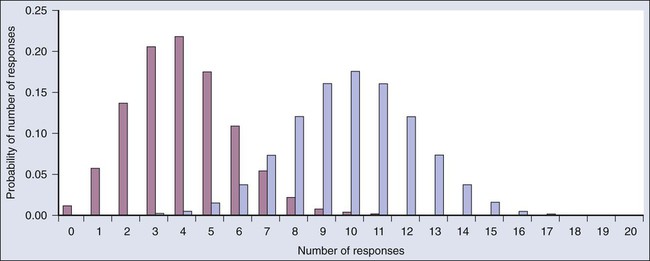
Both the frequentist and Bayesian approaches to clinical trial design and analysis utilize distributions such as those shown in Figure 19-1, but they use them differently.

Frequentist Approach

The frequentist approach to inference is based on error rates. A type I error is rejecting a null hypothesis when it is true, and a type II error is accepting the null hypothesis when it is false, in which case the alternative hypothesis is assumed to be true. It seems reasonable to reject the null, r = 20% (red bars in Fig. 19-1) in favor of the alternative, r = 50% (blue bars in Fig. 19-1) if the number of responses is sufficiently large. Candidate values of “large” might reasonably be where the red and blue bars in Figure 19-1 start to overlap, perhaps nine or greater, eight or greater, seven or greater, or six or greater.

The type I error rates for these rejection rules are the respective sums of the heights of the red bars in Figure 19-1. For example, when the cut point is 9, the type I error rate is the sum of the heights of the red bars for 9, 10, 11, etc., which is 0.007387 + 0.002031 + 0.000462 + … = 0.0100. When the cut points are 8, 7, and 6, the respective type I error rates are 0.0321, 0.0867, and 0.1958. One convention is to define the cut point so that the type I error rate is no greater than 0.05. The largest of the candidate type I error rates that is less than 0.05 is 0.0321, the test that rejects the null hypothesis if there are eight or more responses. The type II error rate is calculated from the blue bars in Figure 19-1, where the alternative hypothesis is assumed to be true. The sum of the heights of the blue bars for 0 up to 7 responses is 0.1316. Convention is to consider the complementary quantity and call it “statistical power:” 0.8684, which rounds off to 87%.

The distinction between “rate” and “probability” in the aforementioned description is important, and failing to discriminate these terms has led to much confusion in medical research.⁵ The “type I error rate” is a probability only when assuming that the null hypothesis is true. Probabilities of events requiring the truth of the null hypothesis are not available in the frequentist approach, and indeed this is a principal contrast with the Bayesian approach (described later).

Suppose the trial is conducted and 9 of 20 patients respond. One concludes that the null, r = 20%, is rejected because 9 is greater than the predetermined cut point of 8. However, the results are more convincing than had the result been exactly 8. Such reasoning led to the convention of reporting a P value, an “observed type I error rate.” This is the type I error rate had the predetermined cut point been set to the observed number. Thus the P value is .0100, as calculated earlier.

Values of r other than 20% and 50% are possible. The standard frequentist approach to representing the range of possibilities is to provide a confidence interval, which is the set of values of r that would not be rejected as null hypotheses based on the data actually observed: 9 responses out of 20 patients (or 45%). For these data, the values of r that would be rejected are those less than 26%. Because very large values of r are also inconsistent with the observed rate of 45%, it is conventional to also exclude large values from the confidence interval. Assuming type I error rates of 5% for both small and large values of r, the resulting confidence interval is from about 26% to 61%, which is a 90% confidence interval in the sense that 5% is excluded on both sides. Excluding only 2.5% on each side provides a 95% confidence interval: 23% to 64%. Ninety-five percent confidence intervals are commonly used and are always somewhat wider than 90% confidence intervals.

Bayesian Approach

A major difference between the Bayesian and frequentist approaches is the use of probability distributions to represent unknown values. In the frequentist approach, probabilities apply only for “data.” Parameters that index data distributions (such as r in the aforementioned example) are unknown but are fixed and thus are not subject to probability statements. In the Bayesian approach, all unknowns, including parameters, have probability distributions.

In the example in which 20 patients yielded 9 responses, suppose that r is assumed to be either 20% or 50%. The Bayesian conclusion is the probability of r = 50%, given the final results. (This is one minus the probability of r = 20% under the assumption that these are the only two possible values of r.) The calculation uses Bayes’ rule. The method is the same as when finding the positive predictive value of a test as it relates to the condition’s prevalence and the test’s sensitivity and specificity. Bayes’ rule is also called the “rule of inverse probabilities” because it relates the probability of some event A given that event B has occurred with the probability of event B given that event A has occurred.

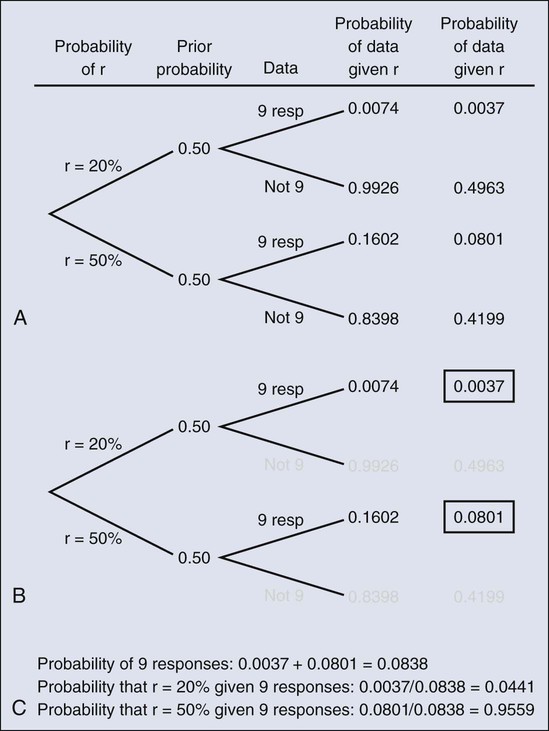
The calculation is intuitive when viewed as a tree diagram, as in Figure 19-2. Figure 19-2, A, shows the full set of probabilities. The first branching shows the two possible parameters, r = 20% and r = 50%. The probabilities shown in the figure, 0.50 for both, will be discussed later. The data are shown in the next branching, with the observed data, nine responses (nine resp) on one branch and all other data on the other. The probability of the data given r, which statisticians call the likelihood of r, is the height of the bar in Figure 19-1 corresponding to nine responses, the red bar for r = 20%, and the blue bar for r = 50%. The rightmost column in Figure 19-2, A, gives the probability of both the data and r along the branch in question. For example, the probability of r = 20% and “nine resp” is 0.50 multiplied by 0.0074.

The probability of r = 20% given the experimental results depends on the probability of r = 20% without any condition, its so-called prior probability. The analog in finding the positive predictive value of a diagnostic test is the prevalence of the condition or disease in question. Prior probability depends on other evidence that may be available from previous studies of the same therapy in the same disease, or related therapies in the same disease or different diseases. Assessment may differ depending on the person making the assessment. Subjectivity is present in all of science; the Bayesian approach has the advantage of making subjectivity explicit and open.⁶

When the prior probability equals 0.50, as assumed in Figure 19-2, the posterior probability of r = 20% is 0.0441. Obviously, this is different from the frequentist P value of 0.0100 calculated earlier. Posterior probabilities and P values have very different interpretations. The P value is the probability of the actual observation, 9 responses, plus that of 10, 11, etc. responses, assuming the null distribution (the red bars in Fig. 19-1). The posterior probability conditions on the actual observation of nine responses and is the probability of the null hypothesis—that the red bars are in fact correct—but assuming that the true response rate is a priori equally likely to be 20% and 50%.

P values are not intuitive in that they condition on a hypothesis that seems unlikely to be true in view of the results (the null hypothesis) and because they depend on probabilities of possible occurrences that were not observed. For example, if there are two candidate null distributions with the same probability of the actual observation, the one with the smaller “tail” of unobserved values will have a smaller P value. Because they are counterintuitive, misinterpretations of P values abound. People usually convert a P value into something they understand but which is wrong, and the misinterpretation usually has a Bayesian ring to it; for example, “The P value is the probability that the results could have occurred by chance alone.” An objection to Bayesian inferences is that they are specific to assumed prior probabilities. A sensible type of report that addresses this concern is the following: “If your prior probability is this, then your posterior probability is that.”

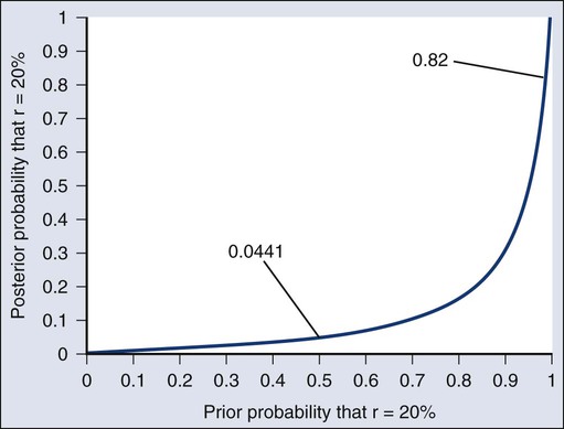
As an example of such a report, Figure 19-3 shows the relationship between the prior and posterior probabilities. The figure indicates that the posterior probability is moderately sensitive to the prior. Someone whose prior probability of r = 20% is 0 or 1 will not be swayed by the data. However, as Figure 19-3 indicates, the conclusion that r = 20% has low probability is robust over a broad range of prior probabilities. A conclusion that r = 20% has moderate to high probability is possible only for someone who was convinced that r = 20% in advance of the trial.

In the example, r was assumed to be either 20% or 50%. It would be unusual to be certain that r is one of two values and that no other values are possible. A more realistic example would be to allow r to have any value between 0 and 1 but to associate weights with different values depending on the degree to which the available evidence supports those values. In such a case, prior probabilities can be represented with a histogram (or density). A common assumption is one that reflects no prior information that any particular interval of values of r is more probable than any other interval of the same width. The corresponding density is flat over the entire interval from 0 to 1 and is shown in red in Figure 19-4, A.

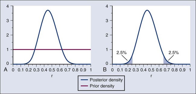
The probability of the observed results (9 responses and 11 nonresponses) for a given r is proportional to r⁹(1-r)¹¹, with the likelihood of r based on the observed results. The prior density is updated by multiplying it by the likelihood. Because the prior density is constant, this multiplication preserves the shape of the likelihood. Thus the posterior density equals just the likelihood itself, shown in green in Figure 19-4, A.

The Bayesian analog of the frequentist confidence interval is called a probability interval or a credibility interval. A 95% credibility interval is shown in Figure 19-4, B: r = 26% to 66%. It is similar to but different from the 95% confidence interval discussed earlier: 23% to 64%. Confidence intervals and credibility intervals calculated from flat prior densities tend to be similar, and indeed they agree in most circumstances when the sample size is large. However, their interpretations differ. A credible interval has a particular probability that the parameter lies in the interval. Statements involving probability or chance or likelihood cannot be made for confidence intervals.

Any interval is an inadequate summary of a posterior density. For example, although r = 45% and r = 65% are both in the 95% credibility interval in the aforementioned example (Fig. 19-4), the posterior density shows the former to be five times as probable as the latter.

A characteristic of the Bayesian approach is the synthesis of evidence. The prior density incorporates what is known about the parameter or parameters in question. For example, suppose another trial is conducted under the same circumstances as the aforementioned example trial, and suppose the second trial yields 15 responses among 40 patients. Figure 19-5 shows the prior density and the likelihoods from the first and second trials. Multiplying likelihood number 1 by the prior density gives the posterior density, as shown in Figure 19-4. This now serves as the prior density for the next trial. Multiplying that density by likelihood number 2 gives the posterior density based on the data from both trials, and is shown in Figure 19-5. The order of observation is not important. Updating first on the basis of the second trial gives the same result. Indeed, multiplying the prior density, likelihood number 1, and likelihood number 2 in Figure 19-5 together gives the posterior density shown in the figure.

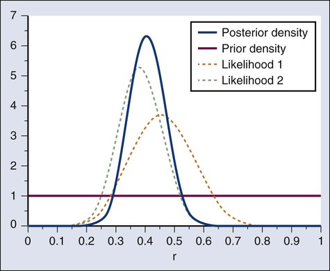
The calculations of Figure 19-5 assume that r is the same in both trials. This assumption may not be correct. Different trials may well have different response rates, say r₁ and r₂. In the Bayesian approach, these two parameters have a joint prior density. One way to incorporate into the prior distribution the possibility of correlated r₁ and r₂ is to use a hierarchical model in which r₁ and r₂ are regarded to be sampled from a probability density that is unknown, and therefore this density itself has a probability distribution. More generally there may be multiple sources of information that are correlated and multiple parameters that have an unknown probability distribution. A hierarchical model allows for borrowing strength across the various sources depending in part on the similarity of the results.^9–9

A rather different application of Bayesian hierarchical models, called a “tumor agnostic,” is destined to become important in cancer clinical trials. Consider an agent targeted at a particular mutation. There may be subsets of patients that harbor this mutation across a broad range of tumor types. The mutation may be rare in some or all tumor types. Mustering a compelling clinical trial in any given tumor type may be impossible. Instead, one might conduct a single trial across ten tumor types, say, regarding response rates r₁, r₂, …, r₁₀ as a sample from a population. The population distribution may be homogeneous, in which case there is substantial “borrowing of strength” across the tumor types. This may enable a claim of effectiveness in tumor types that, when left to stand alone, would have wide credibility intervals because of their small sample sizes. On the other hand, if the population of response rates is heterogeneous, then the observed response rates will be highly variable, and borrowing will occur mainly across neighboring tumor types.

We next apply the Bayesian perspective in two important directions that are the focus of attention in modern cancer research.

Adaptive Designs of Clinical Trials

Randomization was introduced into scientific experimentation by R.A. Fisher in the 1920s and 1930s and applied to clinical trials by A.B. Hill in the 1940s.¹⁰ Hill’s goal was to minimize treatment assignment bias, and his approach changed medicine in a fundamentally important way. The RCT is now the gold standard of medical research. A mark of its impact is that the RCT has changed little during the past 65 years, except that RCTs have gotten bigger. Traditional RCTs are simple in design and address a small number of questions, usually only one. However, progress is slow, not because of randomization but because of limitations of traditional RCTs. Trial sample sizes are prespecified. Trial results sometimes make clear that the answer was present well before the results became known. The only adaptations considered in most modern RCTs are interim analyses with the goal of stopping the trial on the basis of early evidence of efficacy or for safety concerns. There are usually few interim analyses, and stopping rules are conservative. As a consequence, few trials stop early.

In traditional RCTs, randomization proportions are fixed throughout. The possibility that the accumulating data in the trial can influence randomization probabilities or other aspects of a trial’s course may affect the trial’s performance characteristics, including its type I error rate and statistical power. Moreover, these effects may be difficult to analyze using traditional mathematics. However, modern computers and software make traditional mathematics unnecessary. Any prospective trial design, however complicated, can be simulated. A prospective trial design is an automaton. At any time during the trial and based on the information available from trial participants, the next patient is assigned a particular therapy, possibly based on an adaptive randomization scheme. Any trial that has a prospective design can be simulated. Virtual patients can be generated with their outcomes depending on assumed parameter values and treatment assignment according to the prospective design. Replicating the trial 10,000 times, say, gives a firm handle on the trial conclusion for the parameter values assumed in the simulation.

Consider a simple case, a variant of the earlier example in which the response rate r was assumed to be either 20% or 50%. Set the maximum number of patients in the trial to 20. Stop the trial with a claim favoring the alternative hypothesis r = 50% whenever the probability of r = 50% versus r = 20% is at least 95% (and therefore the probability of r = 20% is less than 5%).

As a check that the reader is following this description: the binomial distribution assumed earlier is no longer relevant, even if the final sample size happens to be 20. Consider an extreme case. The binomial distribution gives positive probability to 20 responses regardless of the value of r (unless r = 0). However, the adaptive design would have stopped long before getting to 20 patients when every patient represented a response to the treatment—in fact, the trial would have stopped after four responses in four patients.

It happens that for this simple adaptive design it is possible to find its operating characteristics algebraically, but the calculations are tedious. In more complicated circumstances, algebraic calculations may not be possible and simulations are necessary.

Simulations are easy to describe. To address r = 50%, start with a fair coin, one with probability of heads equal to 50% and interpret “heads” to mean response. Whenever a patient is accrued to the trial, toss the coin, observe the result, and update the probability that r = 50% on the basis of the tosses thus far. Stop the trial if this probability is greater than 95% and make a mark so indicating. If the number of tosses reaches 20 without having made a mark, then stop the trial because you have hit the maximal sample size. When the trial stops, make a note of the total number of tosses, say n, in the trial. Repeat the trial a total of 10,000 times. Count the number of marks and divide by 10,000. This is the estimated power of the study assuming r = 50%. Tabulate the 10,000 values of n to give an estimate of the distribution of the final sample size under the alternative hypothesis. (You should have a mark for every trial with n < 20 and also for some trials with n = 20.)

To find the type I error rate, repeat the aforementioned process with another set of 10,000 iterations generated using a device that has probability of heads equal to 20%. (An example device is a regular 20-sided die with “heads” labeled on four of the sides.) The proportion of marks is the estimated type I error rate. The tabulated values of n are the estimated distribution of the final sample size under the null hypothesis.

Tossing a coin perhaps a hundred thousand times will take a while, especially because you will have to keep track of which trial you are in and whether you have achieved the stopping boundary for that trial. The good news is that a simple program running on a modern desktop computer can simulate 10,000 trials in a few seconds. The computer does all the work. Moreover, an additional few seconds gives you another 10,000 simulated trials assuming another value of r by simply changing the value of r in the program.

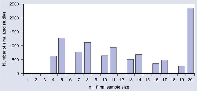
Figure 19-6 shows the sample size distribution for 10,000 trials under the assumption that r = 50%. The estimated type II error rate is 0.1987, which is the proportion of these 10,000 trials that reached n = 20 without ever concluding that the posterior probability of r = 50% is at least 95%. The sample size distribution when r = 20% is not shown but is easy to describe: 9702 of the trials (97.02%) went to the maximum sample size of n = 20 without hitting the posterior probability boundary and the other 3% stopped early (at various values of n < 20) with an incorrect conclusion that r = 50%. Thus 3% is the estimated type I error rate. The “estimated” aspect of these statements is because there is some error due to simulation. Based on 10,000 iterations, the standard error of the estimated power is small, but positive: 0.4%. The standard error of the type I error rate is less than 0.2%.

Because the Bayesian approach allows for updating knowledge incrementally as data accrue, even after every observation, it is ideally suited for building efficient and informative adaptive clinical trials.13–13 The Bayesian approach serves as a tool. As evinced in the example above, simulations enable calculating traditional frequentist measures of type I error rate and power. The Bayesian approach allows for addressing all aspects of drug development: What is the appropriate dose? What is the duration? What are concomitant therapies? What is the sequence? What is the patient subpopulation? Adaptations include dropping arms, adding arms, changing randomization proportions, changing the accrual rate, decreasing or increasing the total sample size, and modifying the patient population admitted to the trial.

Taking an adaptive approach is fruitless when there is no information to which to adapt. In particular, for long-term end points, there may be little information available when making an adaptive decision. However, early indications of therapeutic effect are sometimes available, including longitudinal biomarkers and measurements of tumor burden, for example. These indications can be correlated with long-term clinical outcome to enable better interim decisions.8,13

A limitation of adaptive approaches is that they require the ability to update the outcome database and connect it to the patient assignment algorithm. Another limitation is that an adaptive design, although fully prospective, can be complicated to convey to investigators, patients, institutional review boards, and regulators.

Biomarker-Driven Adaptive Clinical Trials and a Case Study

A standard approach to biomarker research is to examine interactions between biomarkers and treatment effects retrospectively, at the end of the trial. Examining interactions in ongoing clinical trials has many advantages.¹³ One is that requiring biomarker information for randomization means that information will be available for all patients, thus avoiding the “data missingness” problem that plagues retrospective biomarker studies.¹⁴ Another advantage is that when patients in a definable biomarker subset are not benefiting from a particular therapy, that subset can be dropped from the trial. In a multiarmed trial, biomarker subtypes that do not respond to a particular treatment can be excluded from that treatment arm, possibly gradually, using adaptive randomization.¹² A consequence of excluding nonresponders is that focusing on responders means trials can become smaller. And of course, excluding patients who do not benefit reduces the extent of overtreatment of trial participants.

An adaptive biomarker-driven clinical trial can begin by including all the patients who meet the enrollment criteria for the trial, but then can continue by restricting enrollment to individuals with biomarker profiles that match those of the responding population as the results accumulate over the course of the trial. Biomarker subsets can be identified in advance, generated on the basis of the data in the trial, or some combination of the two can be used by incorporating historical data via the prior distribution, as previously described. Any approach is subject to multiplicities.⁵ Basing an assessment on the responding subsets is particularly prone to false-positive conclusions and requires a level of within-trial empirical validation. The extent of validation is a design characteristic that can be determined prospectively. False-positive rates and statistical power can be evaluated and controlled, usually requiring simulations. (Additional evaluations of biomarker-driven adaptive clinical trial designs are available in the literature.^15–18)

An example of a complicated biomarker-driven, adaptively randomized clinical trial is I-SPY 213,19,20 (http://clinicaltrials.gov/show/NCT01042379) (http://www.ispy2.org/). The setting is neoadjuvant treatment for breast cancer in which the end point is pathological complete response (pathCR), which the U.S. Food and Drug Administration (FDA) has recently determined to be a registration end point in high-risk early breast cancer (http://www.fda.gov/downloads/Drugs/GuidanceComplianceRegulatoryInformation/Guidances/UCM305501.pdf). Investigational drugs are added to a taxane in the initial cycles of standard therapy. Similar trials are being explored in other diseases, including lymphoma.²¹

The goal of I-SPY 2 is to efficiently pair drugs and combinations with the patients’ biomarker profiles that characterize the disease subset that responds to that treatment. I-SPY 2 is essentially a screening process. Using Bayesian updating, assignment to therapy is adaptively randomized based on the patient’s tumor biomarkers and the drug’s performance in patients with similar biomarker profiles. A consequence of adaptive randomization is that better-performing drugs move through the process faster. Drugs are graduated when they have a sufficiently high (Bayesian) predictive probability of success in a small, focused phase 3 trial involving patients who are most likely to benefit from the drug based on their biomarker profiles (or the molecular signature of their disease subtype).

The biomarker categories for I-SPY 2 are set in advance and apply to all therapies. The design considers 10 biomarker profiles, or molecular signatures, that make both marketing and biological sense. The categories and signatures are fixed throughout, and any new therapy that is inserted into the trial conforms to the predefined set of biomarker signatures. In a trial similar to I-SPY, the tumor categories could be determined by the drugs’ targets.

Even though the I-SPY 2 end point is ascertained relatively quickly at surgery, waiting 6 months to learn whether a drug is benefiting a particular patient can be a long time. Thus we incorporated magnetic resonance imaging to assess tumor volume after the first cycle of therapy and after the 12 weeks of taxane/investigational drug cycles. Modeling the longitudinal relationship between pathCR and tumor volume reduction enables predicting whether the patient will have a pathCR. Predictions are not perfect, but they help improve the design’s performance. Bayesian modeling appropriately accounts for the uncertainty involved in this prediction process.

Bioinformatics

As a discipline, bioinformatics sits at the interface where biology and medicine meet a confluence of quantitative sciences, including computer science, mathematics, and statistics. Its primary application to oncology is sifting through genome-scale (“omics”) data sets to identify biomarkers and molecular signatures that can be used to predict clinically relevant outcomes. Each omics technology focuses on a particular class of biological molecules: genomics for sequence-based studies of DNA, epigenomics for DNA modifications, transcriptomics for RNA, proteomics for proteins, and metabolomics for small molecules. Predictors that can potentially be used for classification, diagnosis, prognosis, or to select therapy may be found in any of these classes of molecules. The role of bioinformatics is to manage and organize the data and to make possible the statistical analysis needed to discover and validate predictive models based on omics technologies.

Challenges

Numerous challenges must be overcome to incorporate omics data into clinical oncology. The technology changes so rapidly that it can be difficult to develop an assay that will remain stable long enough to discover and validate a model in a clinical trial. A wide variety of omics technologies are available to assay different classes of molecules, which requires researchers and analysts to develop a broad range of expertise, not only in the individual technologies, but also in statistical methods to integrate the resulting data. Omics data sets often are hampered by batch effects, which can be overcome only by careful attention to experimental design and the development of standard protocols. Statistically, the analysis of omics data sets is a struggle against issues of multiple testing and overfitting. The development of second-generation sequencing technologies poses additional challenges from the sheer volume of data and the need for substantial computer power to interpret the data.

The Pace of Technological Change

The first microarrays that could simultaneously measure the messenger RNA (mRNA) expression levels of thousands of genes were developed in the mid 1990s.22,23 Within a few years, they were being used to study cancer.^24–28 The technology evolved rapidly. For example, one of the major manufacturers of microarrays, Affymetrix, began with HuGeneFL GeneChip arrays that contained 6800 probe sets. They advanced over the course of little more than a decade through the U95A (12,000 probe sets), U133A (22,000), U133Plus2.0 (54,000), Human Gene ST 1.0 and 2.0, and Human Exon ST 1.0 and 2.0 microarrays. The typical time between the introductions of successive generations of microarray platforms was 2 or 3 years. Nevertheless, as that decade ended, researchers were increasingly moving away from microarray technology and toward RNA sequencing technology as their primary tool to measure mRNA abundance. The technologies used to measure DNA copy number alterations went through a similar evolution during this period.

This rapid pace of change poses serious challenges when trying to apply these technologies in clinical trials, which may take several years to conduct. Often, the technological platform used to develop a predictive model differs from the one proposed to test the predictions in a clinical trial. It is even possible for a manufacturer to discontinue production of a platform that researchers are using or proposing to use in a clinical trial. Every time the platform changes, the assay must be recomputed and revalidated (preferably by biostatisticians and bioinformaticians working with a laboratory that has been certified according to the Clinical Laboratory Improvement Amendments [CLIA] of the U.S. Code of Federal Regulations).

The Breadth of Technologies

At the same time that microarray technologies were expanding to allow the entire transcriptome to be assayed in a single experiment, new technologies were emerging that focused on other biologically important molecules. The Cancer Genome Atlas (TCGA) recently started assaying approximately 500 tumors per cancer type using a broad spectrum of omics technologies.²⁹ Initial plans called for microarray approaches to measure mRNA expression, microRNA (miRNA) expression, DNA copy number alteration, and methylation. These plans were supplemented by direct Sanger sequencing of a predefined set of cancer-related genes and by proteomic techniques, including mass spectrometry and reverse-phase protein lysate arrays. More recently, TCGA began applying second-generation sequencing technology to study DNA (whole genome or exome sequencing), RNA (RNA-Seq), and methylation (chromatin immunoprecipitation on sequencing, or ChIP-Seq) in these tumor samples.^30,31

In at least one case, an entire class of biologically interesting molecules is itself relatively new. The first miRNA was discovered in 1993 by cloning the lin-4 gene in Caenorhabditis elegans.³² That there were numerous (highly conserved) miRNAs in different species did not become known until the simultaneous publication of three papers in 2001.^35–35 A year later, Calin and colleagues³⁶ demonstrated that miRNAs played an important role in cancer by showing that the “tumor suppressor genes” contained in the minimal deleted region of a recurrent deletion of chromosome 13q in chronic lymphocytic leukemia consisted of miRNA-15a and miRNA-16-1. Version 19 of the reference database, miRBase (http://www.mirbase.org/), maintained by the Wellcome Trust Sanger Institute, now lists 1600 precursors and 2042 mature human miRNAs.^39–39 In addition, of course, there are now microarrays that simultaneously measure (almost) all of them.

Each omics technology requires specialized methods for processing the raw data and converting it into a form that can be analyzed to discover or validate biomarkers and signatures. Often the raw data are fluorescence-based images that must be quantified and summarized. Each assay requires its own form of normalization that is intended to correct for technological artifacts that may distort the measurements. At its simplest, the process of normalization is rescaling the data to account for differences in starting material between samples; if you start an experiment with twice as much total RNA from one sample, then you would expect all of the measurements to be twice as large. More complicated normalization schemes, based on sophisticated statistical models, are common. Bioinformaticians must understand enough about how different biological assays work to select (or develop) appropriate methods to process each kind of data.

Historically, when manufacturers introduced new instruments, they also provided software to quantify and analyze the data that they produced. Statisticians and bioinformaticians, sometimes with good reason, tend to be leery of the “black box” software packages that accompany scientific instruments. For one thing, the structure of the data after quantification, summarization, and normalization is often similar even for radically different technologies, in which case similar statistical methods can be applied. The exact form of the statistical analysis depends less on the nature of the technology platform and more on the design of the experiment. Bioinformaticians must consider several factors, such as the kinds of patient samples that are being contrasted, whether the outcome measures binary, continuous, or time-to-event data, and the covariates (e.g., age, stage, grade, and smoking status) for which they must account in the analysis.

It is unreasonable to expect manufacturers of scientific instruments to have the expertise required to program the wide variety of sophisticated statistical methods needed to account for differences in experimental design. It is surprising, however, that manufacturers do not always know the best ways to process their own raw data. For example, the first Affymetrix microarrays were designed using multiple pairs of “perfect match” and “mismatch” (MM) probes to target each gene. The idea was that the MM probes could be used to estimate nonspecific cross-hybridization, and so their initial algorithm quantified the expression of a gene as the average difference between the perfect match and MM probes. Li and Wong⁴⁰ recognized that different probes for the same gene have different affinities, and thus their mean expression will vary even within the same sample. They replaced the simple average with a statistical model that accounted for different probe affinities.⁴⁰ Bolstad and colleagues⁴¹ and Irizarry and associates⁴² showed that the MM probes increased the noise in the summary measurements with no compensating gain in signal clarity; they introduced an improved statistical method known as the robust multiarray average (RMA). Most current analyses of Affymetrix gene expression data use RMA.

Many advances in the methods for processing and analyzing “omics” data sets have come from academics and are made available as open source software. BioConductor (http://www.bioconductor.org) is the largest repository of such software packages, written for the R statistical programming environment.^43,44 The BioConductor repository is the equivalent of a hardware store for statisticians and bioinformaticians searching for tools with which to analyze their latest data set. An alternative approach is provided by GenePattern⁴⁵ (http://www.broadinstitute.org/cancer/software/genepattern/). GenePattern is a Web service where data can be uploaded and analyzed by biologists as well as statisticians. Modules can be written and shared in a variety of programming languages, then assembled into reusable self-documenting pipelines.

Batch Effects and Experimental Design

Batch effects are an unavoidable characteristic of data collected using cutting-edge technologies on research-grade scientific instruments.⁴⁶ The instruments are often temperamental, requiring frequent tuning and calibration. Reagents change, and new printings of the “same” microarray can be subtly different. As a result, a batch of tumor samples analyzed in November may differ in many ways (although not of biological interest) from a similar batch analyzed in February. These technological effects are often large enough to swamp any interesting biology, and they can occur on the time scale of days rather than months. Unless accounted for in the experimental design, batch effects can ruin a perfectly good experiment. For example, in 2002, Petricoin and colleagues⁴⁷ published an article that claimed they had developed a tool that could be used to diagnose ovarian cancer based on proteomic patterns detected in serum samples. Their results were soon questioned; it eventually transpired that the signals they had detected were technological artifacts, caused by running all of the controls on their mass spectrometer before all of the cases.^50–50

There are several ways to deal with batch effects. First, pay attention to experimental design. Apply the basic principles of randomization and blinding to ensure that the contrasts of interest (tumor vs. normal or responder vs. nonresponder, for example) are not confounded with any batch effects that may be present. Second, if batch effects are suspected, there are existing statistical methods to model them and, to some extent, remove them.53–53

Additional challenges arise in the context of clinical trials. The standard normalization methods for most omics technologies require analyzing the entire set of data at once, which is impossible when patients arrive one by one and a decision about how to randomly assign them to treatment arms depends on the results of an individual assay. In the context of Affymetrix microarrays, this issue was addressed by the introduction of “frozen RMA,” which computes the normalization parameters from a training set and then applies them to new arrays one at a time.⁵⁴ Not all omics technologies have completely faced this issue. In many cases, as with the comparative C_T (or ΔΔC_T) method for quantitative, real-time, reverse-transcription polymerase chain reaction (qPCR),⁵⁵ the best solution may be to run a normalization or calibration standard alongside every experimental sample.

Multiple Testing and Overfitting

At this point, we can assume that we have settled on the technology platform to assay a particular class of biological molecules. We have collected the patient samples, randomized their run order, and corrected any batch effects in the processed data. We are now ready to discover the new biomarkers or molecular signatures that will revolutionize the practice of clinical oncology. And we run head-on into an enormous statistical hurdle: multiple testing.

Each omics technology measures thousands of features simultaneously. (“Feature” is the standard term in the machine learning literature for a potential predictor. The first step in building a complex predictive model is “feature selection”—deciding which features to include and which to leave out of the model. We use the term here for its neutrality; it covers genes, proteins, miRNAs, single nucleotide polymorphisms, enhancers, promoters, or anything else that might help us predict who will or will not respond to a particular therapy.) Each feature can be tested separately for its ability to predict the outcome of interest, and you can associate a P value with each feature in the usual way for the statistical test you are using. However, those P values do not mean what you think they mean. Suppose, for example, that you test 20,000 features and discover that only 1000 of them have P values less than the magic number of .05. In that case, a reasonable conclusion is that nothing you have measured is actually related to the outcome you are trying to predict! The problem is that 1000/20000 = 5%, which is the number of small P values you would expect by chance when performing 20,000 statistical tests.

The traditional statistical response to the problem of multiple testing is to apply a “Bonferroni correction” to the cutoff used to define significance. If you test N features, then the P value should be less than 0.05/N in order for you to claim significance at the 5% level. With 20,000 features, this requirement translates into a P value < .0000025. You probably think that this requirement is extreme, and you may be right. The Bonferroni correction is extremely conservative. It tries to control the “family-wise error rate”; in other words, it attempts to make sure there are no (type I) errors in what you call significant. Continuing our hypothetical experiment, suppose you test 20,000 features and find that 50 of them have a P value <2.5 × 10⁻⁶. In only 5% of such experiments would you expect to find any errors in the list of 50 features. A less conservative approach is to control the false discovery rate (FDR), the expected fraction of false-positive (FP) calls among all positive calls: FP/(FP + TP), where TP is a true-positive call.⁵⁶ Numerous methods have been developed to estimate the FDR in omics experiments.^57–61 A few of these methods also let you estimate the number or rate of false-negative calls. Sometimes called type II errors, false-negative calls have an opportunity cost in terms of potential discoveries that you never make.

Multiple testing becomes much worse when evaluating molecular signatures. First, it is easy to show that random data (created using a random number generator) containing enough “features” can be used to construct a multivariate computational model that will be able to perfectly predict any desired outcome variable on any given set of biological samples. Because the data are random, it is guaranteed that any such model is bogus: it “overfits” the existing data and will not generalize to new data. Second, the P value correction methods that work one feature at a time will not help. For example, the number of 35-feature signatures that can be selected from a set of 10,000 features is approximately a googol (10¹⁰⁰). No molecular signature will ever survive Bonferroni correction of this magnitude. In addition, two different 35-feature signatures that share 30 features in common will be highly correlated, invalidating most of the methods for estimating the FDR. The solution to this problem, however, is simple: any putative predictive model based on a complex signature must be validated on an independent data set, preferably one collected prospectively with respect to the definition of the predictive model.

Sequencing

The move from hybridization-based microarray assays to second-generation sequencing technology poses additional bioinformatics challenges. First, there is the sheer volume of data. Even after discarding the raw images, sequencing data from one sample takes about one terabyte of disk space. Storing these data, moving them across the network, and accessing them efficiently requires improvements in computer hardware and software. Second, raw sequence data requires heavy duty computer processing before it begins to become useful. Millions of sequence “reads” must be mapped to the genome before they can be summarized to provide information about individual genes or other genomic features. In the hybridization approaches, this computational burden is front-loaded and performed once when designing probes. When sequencing, a computational burden exists for every sample processed. Third, because every individual genome is unique, the mapped reads must be interpreted to identify single nucleotide polymorphisms, small insertions and deletions (“indels”), structural variations (translocations or gene fusions), and DNA copy number variation, either present in germline DNA or acquired somatically. Generating the raw sequence data currently takes about a week; mapping and interpreting it may take a month to get through the queue on a high-performance computing cluster.

Best Practices

In response to problems encountered with the premature use of gene-expression signatures in clinical trials at Duke University,⁶² the U.S. Institute of Medicine (IOM) convened a committee to clarify the steps needed to move omics-based signatures from their initial discovery into clinical trials where they can affect patient management and, ideally, improve patient outcomes.⁶³ The most important committee recommendation was to draw a bright line after the discovery and validation of a predictive model and before its application in a clinical trial. Before crossing that line, the test should already be validated, preferably in an independent set of samples or, if that is not available, by cross-validation. A clinical assay should be developed in a CLIA-certified laboratory, and the complete computational procedure must be completely specified and “locked down.” Any change to the procedure requires revalidation of the method before using it to affect patient management. An example is changing the prespecified cutoffs that distinguish patients with high-risk disease from those with low-risk disease; this warrants revalidating the method.

The IOM recommendations build on a long history of related guidelines. For example, the Early Detection Research Network proposed a sequence of phases for the development of biomarkers intended for cancer screening.⁶⁴ However, because the requirements for a good screening biomarker are different from those for a prognostic or predictive biomarker, the Early Detection Research Network biomarker phases are not universally applicable. The minimum information about a microarray experiment (MIAME) standard defines data structures for making microarray data publicly available.⁶⁵ Many journals require authors of papers that use microarray data to deposit them in a public repository (such as the Gene Expression Omnibus or ArrayExpress) using the MIAME standard. The MIAME data structures apply directly to a wide variety of technologies. One weakness of MIAME and related standards like the “minimum information about a proteomics experiment” (MIAPE)⁶⁶ is that, although they describe the collection of metadata about the technology used in an experiment, they do not include a structured way to store clinical or demographic data about the patients whose samples were used in the experiments. Other important guidelines include the reporting recommendations for tumor marker prognostic studies (REMARK),^67,68 the CONSORT statement for randomized trials,⁶⁹ and the STARD initiative for diagnostic studies.⁷⁰

Discovery Phase

The discovery phase lasts from the initial experiments through complete definition of a locked-down computational model to predict an outcome of interest. During this phase, researchers should:

The recommendations to make the data and code available grew out of the problems encountered at Duke University,71,72 but they reflect a larger concern with reproducible research in computationally intensive sciences.^73–76 Because it is impossible to fully understand the biological rationale behind a complex predictive model involving tens or hundreds of genes, it is critically important to be able to confirm that the statistical analysis to discover the model was performed both sensibly and reproducibly. Checking these results requires access to both the original data and the computer code used to analyze it.

The requirement to specify the intended clinical use is also critical. Such information should answer the following questions: In what group of patients will the signature be tested? Will the result of the test be used to screen patients for early diagnosis? Will it provide prognostic information? Will it help select therapy? Will it be used to monitor minimal residual disease or the possibility of recurrence? Different applications require different performance characteristics to demonstrate the usefulness of a biomarker or signature and thus require different experimental designs and different types of controls. Research scientists who have the expertise to develop omics signatures but are not accustomed to designing or running clinical trials can fail to think carefully about these issues. In one example, researchers reported the discovery of peptide patterns with nearly 100% sensitivity and specificity to detect prostate cancer.⁷⁷ The problem was that the cancer specimens came from a group of men with a mean age of 67 years, whereas the control subjects came from a group composed of 58% women, with a mean age of 35 years.⁷⁸

Test Validation Phase

The goal of the test validation phase is to take the locked-down predictive model and turn it into a usable clinical assay. During this phase, researchers should:

We have touched briefly on the need to standardize the assay in our discussion of challenges. The current era of rapidly changing technology and research-grade scientific instruments does not provide the stability needed for a clinical assay. One consequence is that the development of a clinical assay may involve a change of technology. Instead of using microarrays or RNA-Seq to measure gene expression, the assay may be converted to use qPCR. Whole genome sequencing will be replaced by sequencing targeted at a few relevant genes. Tests for DNA copy number alterations may be converted to use fluorescent in situ hybridization. The role of the clinical laboratory is to demonstrate that the assay is analytically reproducible, and, if necessary, to adjust the locked-down predictive model to use the measurements made on the new technology platform.

Evaluation of Clinical Utility

After developing the clinical assay to implement the locked-down predictive model, researchers can start designing the clinical trial. At this point, regulatory issues come into play. As with all clinical trials, researchers must obtain approval from the Institutional Review Board. However, additional action may also be required. In response to a proposed test to detect ovarian cancer (OvaCheck) that grew out of the flawed mass spectrometry experiments on serum, to the clinical trials at Duke, and to similar issues elsewhere, the FDA has ruled that complex predictive models are “medical devices,” the regulation of which falls under their jurisdiction. If those devices will be used in a clinical trial to guide patient management in any way, then researchers must obtain an investigational device exemption (IDE). The IDE is the analog for medical devices of the better-known investigational new drug applications that are needed to test a new drug in a clinical trial. The IOM committee recommends that specific members of the Institutional Review Board should be made responsible for considering the need for an investigational new drug application or IDE in proposed clinical trials.

Not every clinical trial evaluating the utility of a predictive model needs an IDE; the fundamental criterion is whether the molecular signature/assay device is being used to direct patient management. A prospective-retrospective⁷⁹ study design in which the signature is measured on archived specimens to determine whether it would have been useful should not require an IDE. Similarly, a prospective clinical trial in which the signature is passively measured but not used to determine patient care would not need an IDE.

Signatures are Not Enough

In most of the literature, “signature” is a synonym for “list of genes.” As should be clear by this point, having a list of genes is not enough to make predictions about patient outcomes. For that purpose, you must know exactly how to measure each gene, how to combine those measurements to produce a numeric score, and how to interpret that score in a clinical context. Only then do you have a fully specified, locked-down computational model. The good news, however, is that for statistical purposes the fully specified model can be considered to be just one thing. Omics-based predictive signatures are a form of complex biomarker. As a result, the statistical designs for clinical trials that will evaluate one such signature are exactly the same as the designs for evaluating a single biomarker (such as the mutation status of the EGFR gene). The sample size computations are, in principle, identical.

Clustering is Not Prediction

Clustering algorithms, especially in the form of two-way clustered, colored heat maps, have been ubiquitous in the microarray literature since its inception.80,81 Just as a list of genes (a signature) is not enough to make predictions, neither is clustering. There are certainly scientific questions that can be appropriately answered by applying a clustering algorithm; the canonical example involves identifying natural biological subtypes within a larger class of cancer samples. It is, however, possible to identify subtypes with different response profiles. The most likely way to find subtypes related to outcome is to start by performing feature-by-feature statistical tests that identify individual predictors of outcome. After selecting the best predictors, the resulting list of genes (signature!) can be used to cluster the samples. A statistical test can then be performed to determine if the resulting “cluster membership” variable is a good predictor of outcome.

The literature distinguishes between supervised and unsupervised analyses. Supervised methods use the outcome during the analysis; the simplest example is a t-test to identify genes that are differentially expressed between responders and nonresponders. By contrast, clustering is the classical example of an unsupervised approach, because it only uses the gene expression measurements during clustering. However, the procedure described in the previous paragraph is not unsupervised; the process of selecting the best predictive features is a supervised (and essential) part of the procedure.

Two questions illustrate why this clustering procedure, by itself, is inadequate for prediction or classification. First, what happens when you get the data for one new patient? Can you tell to which cluster he or she belongs? Second, how do you validate the clustering results on an independent data set? In both cases, clustering is unable to tell us how to react to new data. Again, this problem has a simple solution. The clustering results must be supplemented by developing a completely specified, locked-down predictive model that assigns new samples to the existing clusters. Not surprisingly, this model will probably use the same features that were selected to perform clustering. After this model is constructed, the predictions can be validated on new data sets and used in prospective clinical trials to classify patients one at a time.

The series of studies performed by Genomic Health to establish its Oncotype DX assay followed most of the procedures recommended by the IOM Committee. First, the researchers asked a well-defined clinical question about a well-defined patient population. Their goal was to predict the risk of distant recurrence after tamoxifen treatment of women with node-negative, estrogen-receptor-positive (ER+) breast cancer. Second, they used four existing microarray data sets from the published literature to select 250 candidate genes. Third, they developed a new assay using qPCR to measure the expression levels of those 250 genes in tumor samples. Fourth, they validated the assay by obtaining data from tumor samples that had been collected in three independent clinical trials of breast cancer, involving a total of 447 women. They performed univariate analyses and selected 23 genes that were associated with the risk of recurrence in at least two out of three qPCR data sets. They then constructed multivariate predictive models and further reduced the set of predictors to a panel of 16 cancer-related genes and five reference genes. Their approach was simple but elegant, reducing a multidimensional problem into a single number, a recurrence score (RS), which made for a straightforward validation process. The algorithm included cutoffs to separate patients into low-, intermediate-, and high-risk categories and was completely specified during this step. Fifth, they tested the prospectively defined qPCR assay and recurrence score algorithm for their ability to predict recurrence in a retrospective set of 668 samples from the National Surgical Adjuvant Breast and Bowel Project (NSABP) B14 trial, for which paraffin blocks were available.⁸² Another study showed that RS did not predict recurrence in women with node-negative breast cancer (regardless of ER status) who had received no adjuvant chemotherapy, which suggests that the signature depends on either the ER positivity or on the treatment.⁸³ Although the RS was built to be prognostic, samples from the NSABP B20 trial showed that it helped predict response to chemotherapy for women with node-negative, ER+ breast cancer, with no apparent benefit for women with low recurrence scores.⁸⁴

BATTLE Trial

The Biomarker-integrated Approaches of Targeted Therapy for Lung Cancer Elimination (BATTLE) trial was a prospective phase 2, biomarker-based, adaptively randomized study in 255 patients who had been pretreated for non–small cell lung cancer (NSCLC).85,86 The trial consisted of four treatment arms of targeted therapies, each of which was associated with a prespecified set of biomarkers that were anticipated to predict the efficacy of the therapy: erlotinib (EGFR), sorafenib (KRAS/BRAF), vandetanib (VEGFR2), and bexarotene plus erlotinib (RXR/CCND1). The primary end point of the trial was 8-week disease control. After an initial equal randomization period, patients were adaptively randomized to one of the treatment arms, based on the molecular biomarkers analyzed in fresh core needle biopsy specimens. Overall results included a 46% 8-week disease control rate, median progression-free survival of 1.9 months (95% confidence interval [CI], 1.8-2.4), and median overall survival of 8.8 months (95% CI, 6.3-10.6). The results confirmed that EGFR mutations predicted better 8-week disease control with erlotinib; high VEGFR2 expression, with vandetanib; and high CCND1 expression, with bexarotene plus erlotinib. The BATTLE study showed that interactions between treatments and biomarkers can be successfully used to guide adaptive randomization.

A follow-up trial, BATTLE-2, is currently under way. This trial also has four treatment arms (sorafenib; erlotinib; erlotinib plus MK2206; and selumetinib plus MK2206) and involves a similar patient population (patients with an EGFR mutation or an EML4-ALK fusion are not eligible for the trial). The fundamental innovation in this trial is that it is divided into two stages in which equal numbers of patients are treated and evaluated. One marker (KRAS mutation) is used, along with observed outcomes, to guide adaptive randomization during the first stage. Twenty prespecified biomarkers or signatures are being measured. At the end of the first stage, a retrospective analysis will be performed to determine the best predictive markers for each treatment arm. These markers will then be used prospectively to guide adaptive randomization in the second half of the trial. Extensive simulations have been performed to determine the operating characteristics of the randomization scheme.⁸⁷

Conclusions

Innovations in cancer research are developing rapidly. The quantitative aspects of this research, from assessing individual genes and biomarkers to evaluating pathways and systems biology, are becoming both more important and more difficult. Assessing which patients benefit from which therapies is the holy grail of cancer research, culminating in clinical trials to demonstrate benefit, or lack thereof. A single adaptive clinical trial can be designed to discover responding subsets and validate the discovery. However, despite the great strides seen in modern cancer biology, strides of much greater magnitude are yet to come. Advances in biology lead to ever more and ever smaller subsets. Large clinical trials will soon be impossible, and traditional statistical approaches will have to be replaced. We cannot predict what those will be. Our aim has been to describe some ways the scientific winds are blowing, preparing the reader to understand and appreciate the path being followed.