[level-membership-for-orthopaedics-category]Chapter 13
Research Design and Biostatistics
SECTION 2 COMMON RESEARCH DESIGNS AND research TERMINOLOGY
IV. Observational Research Designs
VI. Experimental Research Designs
SECTION 3 THE LEVELS OF EVIDENCE IN ORTHOPAEDIC RESEARCH
SECTION 4 CONCEPTS OF EPIDEMIOLOGY
SECTION 5 STATISTICAL METHODS FOR TESTING HYPOTHESES
section 2 Common Research Designs and Research Terminology
A Designed to assess outcomes occurring forward in time
B Exposure has occurred or risk factor has developed; patients are monitored forward in time to determine the occurrence of an outcome of interest.
A Designed to assess outcomes that have already occurred or data that has been collected in the past
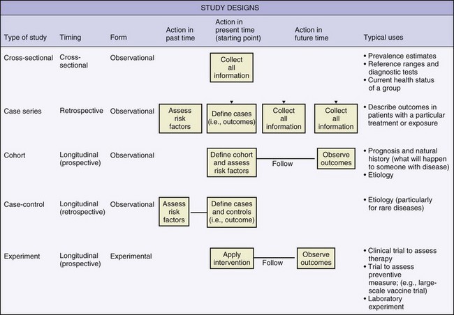
IV OBSERVATIONAL RESEARCH DESIGNS
These designs can be prospective, retrospective or longitudinal (Figures 13-1 and 13-2). Common observational designs are as follows:


1. Descriptions of unique injures, disease occurrences, or outcomes in a single patient
2. No attempts at advanced data analysis are made.
3. Cause-effect relationships are not discussed, and generalizations are not made.
1. Outcomes are measured in patients with a particular disease or injury.
2. In orthopaedic research, these studies are typically retrospective and involve a thorough review of medical records.
1. Outcomes measured in patients with a particular disease or injury are compared with outcomes in a control group (see subsection VII, Potential Problems with Research Designs, for more information about control groups).
2. Odds ratios (not relative risks) are appropriate measures of association from data collected in these study designs (see Section 4, Concepts of Epidemiology).
1. An instrument’s ability to accurately describe truth or reality
2. In a validation study, measurements recorded by a particular instrument are tested against a “gold standard” measure.
1. The ability to precisely describe a characteristic with repeated measurements
2. The precision of an instrument can be tested by different examiners on the same patient (interobserver reliability) or by the same examiner at consecutive times (intraobserver reliability).
3. The intraclass correlation coefficient is a common statistical method for testing the reliability or validity of an instrument. Values range from 0 to 1.0 (1.0 represents perfect accuracy or precision).
C Clinical studies can be designed to determine superiority of one treatment over another, whether one treatment is no worse than another (noninferiority), or whether both treatments are equally effective (equivalency).
D Clinical research can be designed to assess outcomes data that are reported by the patient (subjective) or collected by an examiner (objective).
VI EXPERIMENTAL RESEARCH DESIGNS
A Clinical trials: allocate treatments and track outcomes in order to test a specific hypothesis
1. The clinical trial that is the “gold standard” and is based on the highest level of evidence is the randomized controlled trial.
B Parallel designs: Treatments are allocated to different subjects or patients in a random or nonrandom manner.
C Crossover designs: Each subject receives or undergoes a series of treatments of each treatment condition being studied.
VII POTENTIAL PROBLEMS WITH RESEARCH DESIGNS
A Internal validity concerns the quality of a research design and how well the study is controlled and can be reproduced. External validity concerns the ability of the results to generalize to a whole population of interest.
B Confounding variables are factors extraneous to a research design that potentially influence the outcome. Conclusions regarding cause-effect relationships may be explained by confounding variables, instead of by the treatment or intervention being studied and must therefore be controlled or accounted for.
C Bias is unintentional, systematic error that threatens the internal validity of a study. Sources of bias include selection of subjects (sampling bias), loss of subjects to follow-up (nonresponder bias), observer/interviewer bias, and recall bias.
D Protection against these threats can be achieved through randomization (i.e., random allocation of one or more treatments) to ensure that bias and confounding factors are distributed equally among the study groups. Single blinding (examiner or patient is unaware of to which study condition the patient is assigned) or double blinding (both examiner and patient are unaware of assignment of study condition) is important for minimizing bias.
E Control groups can help account for the potential placebo effect of interventions.
1. Control groups may receive an intervention that reflects the standard of care, no intervention, a placebo (i.e., inactive substance), or a sham intervention.
2. Control data may have been collected in the past (historical controls) or may occur in sequence with one or more other study interventions (crossover design).
F Control subjects are often matched on the basis of specific characteristics (e.g., gender, age), which helps account for potential confounding variables that may influence the interpretation of research findings.
G The strongest research design involves the use of random allocation, blinding, and use concurrent control subjects who are matched to the experimental group(s).
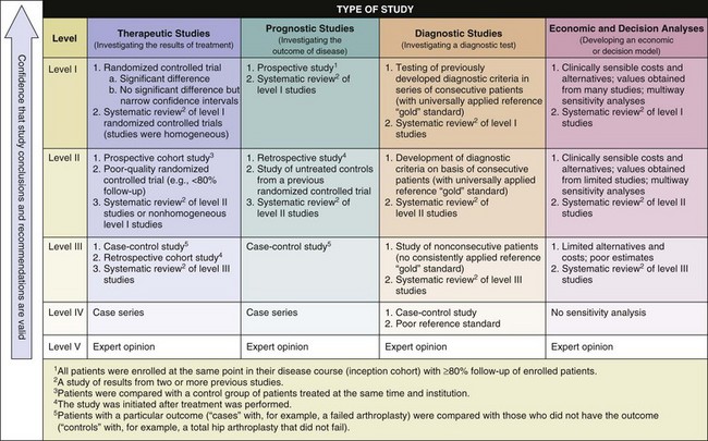
section 3 The Levels of Evidence in Orthopaedic Research
A Evidence-based medicine (or evidence-based practice) aims to apply evidence from the highest quality research studies to the practice of medicine.
B Findings from the best designed and most rigorous studies have the greatest influence on decision making.
section 4 Concepts of Epidemiology
A Prevalence is the proportion of existing cases or conditions of injuries or disease within a particular population.
B Incidence (absolute risk) is the proportion of new injuries or disease cases within a specified time interval (a follow-up period is required).
1. The incidence can be reported with regard to the number of exposures.
2. Example: Of 100 athletes on a sports team, 12 experience a sports-related injury during a 10-game season; the incidence rate would be reported as 12 injuries per 1000 athlete exposures.
D Relative risk (RR) is a ratio between the incidences of an outcome in two cohorts. Typically, a treated or exposed cohort (in the numerator of the ratio) is compared with an untreated or unexposed (control) group (in the denominator of the ratio). Values can range from 0 to infinity and are interpreted as follows:
1. When RR = 1.0, the incidence of an outcome is equal between groups.
2. When RR > 1.0, the incidence of an outcome is greater in the treated/exposed group (higher incidence value in the numerator).
3. When RR < 1.0, the incidence of an outcome is greater in the untreated/unexposed group (higher incidence value in the denominator).
E Odds ratios are calculated from the probabilities of an outcome in two cohorts.
1. Odds ratios are well suited for binary data or studies in which only prevalence can be calculated.
F Interpreting relative risk and odds ratio:
1. Odds ratio and relative risk values are interpreted similarly.
2. When outcomes of two groups are compared, a relative risk or odds ratio of 0.5 would indicate that the likelihood that the treated/exposed patients will experience a particular outcome is half that of the untreated/control group.
3. A value of 2.5 would indicate that the likelihood that the treated/exposed group will experience the outcome is 2.5 times higher than that of the untreated/control group.
II CLINICAL USEFULNESS OF DIAGNOSTIC TESTS
A 2×2 contingency table (Figure 13-3) can be used to plot the occurrences of a disease or outcome of interest among patients whose diagnostic test results were positive or negative.
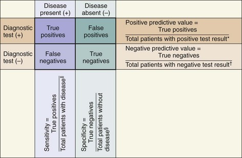

1. “True positives”: the number of individuals whose diagnostic test yielded positive results and who actually do have the disease or outcome of interest
2. “True negatives”: the number of individuals whose diagnostic test yielded negative results and who actually do not have the disease or outcome of interest
3. “False positives”: the number of individuals whose diagnostic test yielded positive results but who actually do not have the disease or outcome of interest
4. “False negatives”: the number of individuals whose diagnostic test yielded negative results but who actually do have the disease or outcome of interest
B Analysis of diagnostic ability
 The likelihood of a positive test result in patients who actually have the disease or condition of interest (i.e., ability to detect true positives among those with a disease)


 The likelihood of a negative test result in patients who actually do not have the disease or condition of interest (i.e., ability to detect “true negatives” among those without a disease)


 The proportion of patients with a positive test result actually has the disease or condition of interest


 The proportion of patients with a negative test result actually does NOT have the disease/condition of interest


 Probability that a disease exists, according to a test result. Likelihood ratios account for both specificity and sensitivity of a given test.
 Likelihood ratios close to 1.0 provide little confidence regarding the presence or absence of a disease.


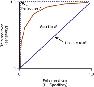
6. Receiver operating characteristic (ROC) curves are graphic representations of the overall clinical utility of a particular diagnostic test that can be used to compare accuracy of different tests in diagnosing a particular condition (Figure 13-4).


section 5 Statistical Methods for Testing Hypotheses
Statistical tests match the purpose of a particular research study. Statistical analyses differ according to the goals of the researcher: for example, to compare groups to identify differences or establish relationships between groups (Table 13-1).
Table 13-1
| Desired Analysis | Parametric Statistics* | Nonparametric Statistics† |
| Comparison of two groups | ||
| Paired | Dependent (paired)–samples t-test | Wilcoxon test |
| Unpaired | Independent-samples t-test* | Mann-Whitney U test |
| Comparison of three or more groups | ||
| One outcome variable | Analysis of variance (ANOVA) | Kruskal-Wallis test |
| Repeated observations in same patient | Repeated-measures ANOVA | Friedman test |
| Multiple dependent variables | Multivariate analysis of variance (MANOVA) | |
| Analysis including a covariate | Analysis of covariance (ANCOVA) | |
| Establishing relationship or association | Pearson product-moment correlation coefficient | Spearman rho correlation coefficient |
| Prediction | ||
| From one predictor variable | Simple regression | Logistic regression |
| From two or more predictor variables | Multiple regression | |
| Comparisons of categorical data | ||
| Two or more variables | Chi-square | Chi-square |
| Better for low sample size | Fisher exact test | Fisher exact test |
*Appropriate for normally distributed continuous data.
†Alternative tests appropriate for nonnormally distributed data, small sample sizes, or both.
I SAMPLING AND GENERAL TERMINOLOGY
A A population consists of all individuals who share a specific characteristic of clinical or scientific interest. Parameters describe the characteristics of a population.
B Study samples affords all members of a specific population equal chance of being studied or enrolled in a clinical study.
C Sample populations are representative subsets of the whole population. Statistics describe the characteristics of a sample and are intended to be generalized to the whole population.
D Populations are delimited on the basis of inclusion and exclusion criteria that are established before a study starts.
E Types of data collected from samples:
1. Discrete data have an infinite number of possible values (e.g., age, height, distance, percentages, time)
2. Categorical data have a limited or finite number of possible values or categories (e.g., excellent, good, fair, or poor; male or female; satisfied or unsatisfied).


F Data can be plotted in frequency distributions (histograms) to summarize basic characteristics of the study sample.
G Cutoff points: Continuous data are often converted into categorical or binary data through the use of cutoff points. Cutoff points can be arbitrary or evidence based.
1. In evidence-based establishment of cutoff points, ROC curves are used, and a point that maximizes sensitivity, specificity, or both of a particular test is identified.
2. Example: A numerical value can be established as a cutoff point for white blood cell count to identify whether an infection exists.
3. Arrays of continuous data can be separated into percentiles to identify upper and lower halves, thirds, quartiles, and so forth.
A A data distribution histogram describes the frequency of occurrence of each data value. Distributions can be described in descriptive statistics such as the following:
1. Mean is calculated as the sum of all scores divided by the number of samples (n).
2. Median is the value that separates a dataset into equal halves; half of the values are higher and half are lower than the median.
3. Mode is the most frequently occurring data point.
4. Range is the difference between the highest value and the lowest value in a dataset.
5. Standard deviation is a value that describes the dispersion or variability of the data.

B Characteristics of a dataset (Figure 13-5):
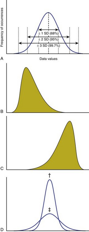
1. Normally distributed data appear in a graph as a bell-shaped curve. The mean, median, and mode are the same value in a gaussian (normal) distribution.
2. Skewed data distributions are asymmetric and may be caused by outliers. Data distributions can be skewed to the left (negative skew) or skewed to the right (positive skew).
3. Kurtosis is a measure of the relative concentration of data points within a distribution. If data values cluster closely, the dataset is more kurtotic.
4. Outliers are data points that are considerably different from the rest of the dataset. Outliers can cause data distributions to be skewed.
C Confidence intervals quantify the precision of the mean or of another statistic, such as an odds ratio or relative risk.
1. Confidence intervals are calculated to provide a range of values around a point estimate (such as a mean, proportion, relative risk, or odds ratio) that can be used to describe the level of confidence that the study data represent the truth.
2. Datasets that are highly variable (have large standard deviations) have larger confidence intervals and hence enable less accurate estimates of the characteristics of a population.
3. A 95% confidence interval consists of a range of values within which researchers are 95% certain that the actual population parameter (e.g., mean, odds ratio, relative risk) is located.

A Inferential statistics are used to test specific hypotheses about associations or differences among groups of subject or sample data.
B The dependent variable is what is being measured as the outcome. There can be multiple dependent variables, depending on how many outcome measures are desired.
C The independent variables include the conditions or groupings of the experiment that are systematically manipulated by the investigator.
1. For example, a researcher is measuring pain and prescription medication use in patients with shoulder pain who are receiving treatment A, B, or C. The dependent variables are pain and prescription medicine use. The independent variable is treatment condition, of which there are three (A, B, and C).
D Inferential statistics can be generally divided into parametric and nonparametric statistics.
1. Parametric inferential statistics are appropriate for continuous data and rely on the assumption that data are normally distributed.


2. Nonparametric inferential statistics are appropriate for categorical and data that are not normally distributed.
 The median and ranks are used in calculating these statistics, and the statistics are therefore more robust alternatives when data are not normally distributed.
3. The goal of inferential statistics is to estimate parameters.


A Some important distinctions:
1. How many groups are being studied
2. Whether the measures are being recorded in the same or different subjects
B When two groups of data are compared, the t-test is used. There are two variations of the t-test:


C When three or more groups are compared, an analysis of variance is used. This is also known as the F-test.
1. Analysis of variance (ANOVA) is appropriate when three or more groups of continuous, normally distributed data are used.

2. Repeated-measures ANOVA is a variation of the ANOVA that is appropriate for sequential measurements recorded from the same subjects.
 For example, this test would be used to compare a dependent variable (outcome measure) recorded at three or more time points (e.g., baseline, 1 month after intervention, 2 months after intervention).

3. Multivariate analysis of variance (MANOVA), a variation of the ANOVA, is used when multiple dependent variables are compared among three or more groups.
4. Analysis of covariance (ANCOVA) is an appropriate test when confounding factors must be accounted for in the statistical analysis.
5. Post hoc testing is necessary after any ANOVA to determine the exact location of differences among groups.
 ANOVAs describe whether a statistically significant difference exists in some way among the study groups.
 For example, when three levels of the independent variable—treatment conditions A, B, and C—are compared, post hoc testing involves specific comparisons of conditions A and B, conditions B and C, and conditions A and C to determine the exact type of group differences. Post hoc testing is appropriate only if the ANOVA yields statistically significant findings (see Section 6, Important Concepts in Research and Statistics).
 Common post hoc tests: Tukey Honestly Significant Difference, Sidak, Dunnet, and Scheffe
6. Factorial designs are used for multiple independent variables.


 These describe the strength of a relationship between two variables.
 The Pearson product correlation coefficient (r) used for continuous, normally distributed data.


 This statistic describes the ability of one independent (predictor) variable to predict a dependent (outcome) variable.

 R2 ranges from 0 to 1.0, whereby higher values indicate more variance explained.
3. Multivariate linear regression describes the ability of several independent variables to predict a dependent variable.
4. Logistic regression is used when the outcome is categorical and the predictor variables can be either categorical or continuous data that are not normally distributed.


section 6 Important Concepts in Research and Statistics
A Type I error (α error, false-positive error)
1. The probability that a statistical test result is wrong when the null hypothesis is rejected (e.g., the finding that groups are different when they actually are not).
2. It is accepted that this error may occur 5 times out of 100 tests; therefore, the probability value threshold for statistical significance is 0.05, or 5%.
A Inferential test statistics (e.g., t statistic, F statistic, r coefficient) are accompanied by a probability (P) value. These values are on a scale from 0% to 100% and indicate the probability that the differences or relationships among study data occurred by chance.
B P values less than 0.05 mean there is less than a 5% chance that the observed difference or relationship has occurred by chance alone and not because of the study intervention.
C Typical threshold for “statistical significance”: P value = 0.05 or less (type I error may occur in 5 of 100 tests)
1. The decision regarding the threshold for defining statistical significance is arbitrary, but this α level (type I error) is generally accepted.
D Therefore, in accordance with the P value, the null hypothesis—which is that no differences or no association exists either is rejected (i.e., P < 0.05) or fails to be rejected (P > 0.05)

III STATISTICAL POWER AND ESTIMATING SAMPLE SIZE
A Research studies should have enough subjects or samples in order to obtain valid results that can be generalized to a population while minimizing unnecessary risk.
B Sample size estimates are based on the desired statistical power (these estimates are often termed power analyses).
1. Statistical power is the probability of finding differences among groups when differences actually exist (i.e., avoiding type II error).
2. These differences are desirable in 80% or more of statistical tests.
C Sample sizes are justified as the number of subjects needed for researchers to find a statistically significant difference or association (i.e., P ≤ 0.05) while statistical power is maintained higher than 80%.
D Higher sample sizes or highly precise measurements (lower variability) are necessary to find small differences between study groups.
E Power analyses can be done before the study starts (a priori) or after the study has been completed (post hoc).
1. Studies with low power have a higher likelihood of missing statistical differences when they actually exist (i.e., type II error).
2. To understand the power of a statistical test, the following aspects should be considered: the number of subjects in the study, the effect size (see subsection V, Effect Sizes), the acceptable level of type I error (usually 5%; i.e., P ≤ 0.05), and an estimate of variability in the data.
3. The power of statistical tests (which improve the likelihood of finding statistical differences when they exist) increases with more subjects, greater treatment effect, and lower variability among the data.
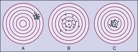
4. Researchers often design studies to maximize the potential for response to a particular treatment by using stringent inclusion and exclusion criteria and selecting a measurement device or outcome instrument that is more precise and accurate (Figure 13-6).
IV MINIMAL CLINICALLY IMPORTANT DIFFERENCES
A Describe the least change in a patient-oriented outcome measure that would be perceived as being beneficial to the patient or would necessitate treatment.
B Statistical significance does not imply clinical importance.
C Many of the patient-oriented outcome instruments that are more commonly used have research-established minimal clinically important difference values.
D Clinicians should consider whether observed differences are important enough to change practice.
A Used to describe the magnitude of a treatment effect. An example is Cohen’s d effect size.
B Calculated as the difference between treatment groups divided by the standard deviation (typically pooled standard deviation, or the standard deviation of the reference or control group).
C Interpretation: Effect sizes greater than 0.8 are “strong”; those less than 0.2 are “small” (between these values can be interpreted as “medium”)
Kocher, MS, Zurakowski, D. Clinical epidemiology and biostatistics: a primer for orthopaedic surgeons. J Bone Joint Surg Am. 2004;86:607–620.
Wang, D, et al. A primer for statistical analysis of clinical trials. Arthroscopy. 2003;19:874–881.
Wright, JG, et al. Introducing levels of evidence to the journal. J Bone Joint Surg Am. 2003;85:1–3.
1. A research study includes chart reviews of patients who underwent a partial knee arthroplasty, and these reviews are compared with those of osteotomy recipients who were of the same age and weight and had the same level of arthritis. This study would best be described as:
3. In epidemiology studies, “incidence” is:
A The proportion of individuals with a disease right now
B The rate of the new occurrences of a disease per unit of time
C The proportion of a sample population with a disease under study
D Variability occurring between successive observations by the same surgeon
E Variability occurring between observations by different surgeons
4. During clinical follow-up, a subjective pain rating from two unmatched groups of patients with chronic patellofemoral joint pain is collected. One of the groups received a surgical intervention, and the other received conservative management. The purpose of the study is to compare subjective pain rating between the two groups. Which of the following statistical tests is most appropriate?
5. A statistical test is associated with a P value of 0.04. What is the interpretation of this value?
A There is 4% chance of being wrong when the test is described as “statistically significant.”
B There is 4% chance of being correct when the test is described as “statistically significant.”
C The type II error is excessive.
D The study has insufficient statistical power.
E There is a 96% chance that the test is clinically important.
[/level-membership-for-orthopaedics-category][not-level-membership-for-orthopaedics-category]Chapter 13
Research Design and Biostatistics
SECTION 2 COMMON RESEARCH DESIGNS AND research TERMINOLOGY
IV. Observational Research Designs
VI. Experimental Research Designs
SECTION 3 THE LEVELS OF EVIDENCE IN ORTHOPAEDIC RESEARCH
SECTION 4 CONCEPTS OF EPIDEMIOLOGY
SECTION 5 STATISTICAL METHODS FOR TESTING HYPOTHESES
section 2 Common Research Designs and Research Terminology
A Designed to assess outcomes occurring forward in time
B Exposure has occurred or risk factor has developed; patients are monitored forward in time to determine the occurrence of an outcome of interest.
A Designed to assess outcomes that have already occurred or data that has been collected in the past
IV OBSERVATIONAL RESEARCH DESIGNS
These designs can be prospective, retrospective or longitudinal (Figures 13-1 and 13-2). Common observational designs are as follows:
1. Descriptions of unique injures, disease occurrences, or outcomes in a single patient
2. No attempts at advanced data analysis are made.
3. Cause-effect relationships are not discussed, and generalizations are not made.
1. Outcomes are measured in patients with a particular disease or injury.
2. In orthopaedic research, these studies are typically retrospective and involve a thorough review of medical records.
1. Outcomes measured in patients with a particular disease or injury are compared with outcomes in a control group (see subsection VII, Potential Problems with Research Designs, for more information about control groups).
2. Odds ratios (not relative risks) are appropriate measures of association from data collected in these study designs (see Section 4, Concepts of Epidemiology).
1. An instrument’s ability to accurately describe truth or reality
2. In a validation study, measurements recorded by a particular instrument are tested against a “gold standard” measure.
1. The ability to precisely describe a characteristic with repeated measurements
2. The precision of an instrument can be tested by different examiners on the same patient (interobserver reliability) or by the same examiner at consecutive times (intraobserver reliability).
3. The intraclass correlation coefficient is a common statistical method for testing the reliability or validity of an instrument. Values range from 0 to 1.0 (1.0 represents perfect accuracy or precision).
C Clinical studies can be designed to determine superiority of one treatment over another, whether one treatment is no worse than another (noninferiority), or whether both treatments are equally effective (equivalency).
D Clinical research can be designed to assess outcomes data that are reported by the patient (subjective) or collected by an examiner (objective).
VI EXPERIMENTAL RESEARCH DESIGNS
A Clinical trials: allocate treatments and track outcomes in order to test a specific hypothesis
1. The clinical trial that is the “gold standard” and is based on the highest level of evidence is the randomized controlled trial.
B Parallel designs: Treatments are allocated to different subjects or patients in a random or nonrandom manner.
C Crossover designs: Each subject receives or undergoes a series of treatments of each treatment condition being studied.
VII POTENTIAL PROBLEMS WITH RESEARCH DESIGNS
A Internal validity concerns the quality of a research design and how well the study is controlled and can be reproduced. External validity concerns the ability of the results to generalize to a whole population of interest.
B Confounding variables are factors extraneous to a research design that potentially influence the outcome. Conclusions regarding cause-effect relationships may be explained by confounding variables, instead of by the treatment or intervention being studied and must therefore be controlled or accounted for.
C Bias is unintentional, systematic error that threatens the internal validity of a study. Sources of bias include selection of subjects (sampling bias), loss of subjects to follow-up (nonresponder bias), observer/interviewer bias, and recall bias.
D Protection against these threats can be achieved through randomization (i.e., random allocation of one or more treatments) to ensure that bias and confounding factors are distributed equally among the study groups. Single blinding (examiner or patient is unaware of to which study condition the patient is assigned) or double blinding (both examiner and patient are unaware of assignment of study condition) is important for minimizing bias.
E Control groups can help account for the potential placebo effect of interventions.
1. Control groups may receive an intervention that reflects the standard of care, no intervention, a placebo (i.e., inactive substance), or a sham intervention.
2. Control data may have been collected in the past (historical controls) or may occur in sequence with one or more other study interventions (crossover design).
F Control subjects are often matched on the basis of specific characteristics (e.g., gender, age), which helps account for potential confounding variables that may influence the interpretation of research findings.
G The strongest research design involves the use of random allocation, blinding, and use concurrent control subjects who are matched to the experimental group(s).
section 3 The Levels of Evidence in Orthopaedic Research
A Evidence-based medicine (or evidence-based practice) aims to apply evidence from the highest quality research studies to the practice of medicine.
B Findings from the best designed and most rigorous studies have the greatest influence on decision making.
section 4 Concepts of Epidemiology
A Prevalence is the proportion of existing cases or conditions of injuries or disease within a particular population.
B Incidence (absolute risk) is the proportion of new injuries or disease cases within a specified time interval (a follow-up period is required).
1. The incidence can be reported with regard to the number of exposures.
2. Example: Of 100 athletes on a sports team, 12 experience a sports-related injury during a 10-game season; the incidence rate would be reported as 12 injuries per 1000 athlete exposures.
D Relative risk (RR) is a ratio between the incidences of an outcome in two cohorts. Typically, a treated or exposed cohort (in the numerator of the ratio) is compared with an untreated or unexposed (control) group (in the denominator of the ratio). Values can range from 0 to infinity and are interpreted as follows:
1. When RR = 1.0, the incidence of an outcome is equal between groups.
2. When RR > 1.0, the incidence of an outcome is greater in the treated/exposed group (higher incidence value in the numerator).
3. When RR < 1.0, the incidence of an outcome is greater in the untreated/unexposed group (higher incidence value in the denominator).
E Odds ratios are calculated from the probabilities of an outcome in two cohorts.
1. Odds ratios are well suited for binary data or studies in which only prevalence can be calculated.
F Interpreting relative risk and odds ratio:
1. Odds ratio and relative risk values are interpreted similarly.
2. When outcomes of two groups are compared, a relative risk or odds ratio of 0.5 would indicate that the likelihood that the treated/exposed patients will experience a particular outcome is half that of the untreated/control group.
3. A value of 2.5 would indicate that the likelihood that the treated/exposed group will experience the outcome is 2.5 times higher than that of the untreated/control group.
II CLINICAL USEFULNESS OF DIAGNOSTIC TESTS
A 2×2 contingency table (Figure 13-3) can be used to plot the occurrences of a disease or outcome of interest among patients whose diagnostic test results were positive or negative.
1. “True positives”: the number of individuals whose diagnostic test yielded positive results and who actually do have the disease or outcome of interest
2. “True negatives”: the number of individuals whose diagnostic test yielded negative results and who actually do not have the disease or outcome of interest
3. “False positives”: the number of individuals whose diagnostic test yielded positive results but who actually do not have the disease or outcome of interest
4. “False negatives”: the number of individuals whose diagnostic test yielded negative results but who actually do have the disease or outcome of interest
B Analysis of diagnostic ability
The likelihood of a positive test result in patients who actually have the disease or condition of interest (i.e., ability to detect true positives among those with a disease)
The likelihood of a negative test result in patients who actually do not have the disease or condition of interest (i.e., ability to detect “true negatives” among those without a disease)
The proportion of patients with a positive test result actually has the disease or condition of interest
The proportion of patients with a negative test result actually does NOT have the disease/condition of interest
[/not-level-membership-for-orthopaedics-category]
