Chapter 6 Radiation Oncology Physics
In the irradiation of a biologic system, physical and biologic events occur in the following order:
Matter and Physical Definitions
Atomic and Nuclear Structure, Particles, and Nomenclature
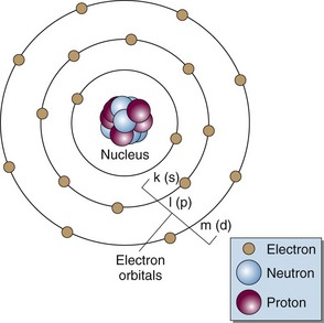
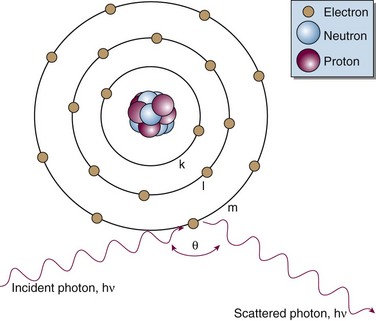
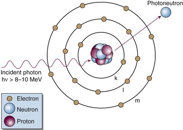
Matter is made up of atomic and nuclear particles that have interaction and binding energies from 1 to 10 million electron volts (MeV). The smallest structural subunit that retains the character of an element, the atom, has a nucleus consisting of one or more protons and zero or more neutrons and a surrounding cloud of orbiting electrons. In an atom with zero net electrical charge, the number of orbital electrons equals the number of protons. A simplistic representation shows the atom to be neatly arranged with neutrons and protons in the nucleus and electrons in uniform orbits (Fig. 6-1). In reality, the atom is a dynamic structure with defined energy states for the electron orbits and the nucleus. Detailed atomic and nuclear models have been formalized.1,2
Neutrons and protons are the building blocks of the nucleus; hence, they are called nucleons. The two particles have similar rest masses (the mass of the particle at rest, when kinetic energy is zero) but different electrical charges. The neutron, symbolized by n, has no charge (neutron for neutral) and the proton, p, has a charge of +1. The electron, e, has an atomic mass about  that of a proton or neutron and has a charge of −1. Besides the neutron, proton, and electron, other particles exist with unique masses and properties (e.g., spin). These include neutrinos, pions, muons, and others. The neutrino was first proposed as the neutral accompanying particle emitted in beta decay. There has been great interest in determining the mass of the neutrino because the cumulative neutrino mass may account for the “missing mass” in the Universe, with great cosmologic implications. More recently it has been determined that the neutrino mass, inferred through observed oscillations in the neutrino state,3,4 is finite and also very small (close to zero). However, even with nonzero mass the total amount of neutrino mass is estimated to be insufficient to make up for the “missing” mass. The Universe is now stated to be made up of matter (4.6% the material “stuff” we are familiar with), dark matter (23%), and dark energy (which comprises over 70% of the total mass-energy content of the Universe).5 These “dark” components are unknown entities.
Particles are classified by their mass as leptons or hadrons. Leptons, which include the electron and neutrino, are “lightweight” particles with mass comparable to that of the electron and spin of  . Hadrons are heavy particles with two subclasses called mesons (middleweight, spin 0 or 1) and baryons (heavyweight, spin
  or
or  ). Fundamental, or elementary, particles are those that have no subparts and cannot be divided. All leptons are elementary particles; however, the neutron and proton are not and are instead made up of three fundamental particles each, called quarks, which have been observed through high-energy physics experiments. Quarks have positive or negative charge in integer increments of
  , spin of
  , and other properties with whimsical, quark-deserving names.1 Combinations of quarks yield the neutron, proton, and all other hadrons. For instance, a proton is made of two up quarks and one down quark, whereas a neutron is made of one up and two down quarks, which explains their similar mass but difference in charge. Antimatter is real, and an antiparticle is defined as a particle with identical mass but opposite charge to the particle. An antiparticle for a neutral particle has opposite spin or internal charge (i.e., quark) compared with the particle.
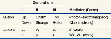
Matter is held together by four fundamental forces that operate over certain ranges and with certain particles. They are the strong, electromagnetic (coulomb [C]), weak, and gravitational forces, with respective relative strengths of 101, 10−2, 10−13, and 10−42.1 Each force acts by exchange of its respective mediator particle: the gluon, the photon, the W and Z particles, and the graviton. Counting mediators, leptons, hadrons, and their antiparticles, there are about 170 fundamental and composite particles that make up matter.1 The model in which matter consists of fundamental particles as described earlier is called the standard model.1 Table 6-1 summarizes the fundamental particles in the standard model, which are six quarks, six leptons, six antiquarks, six antileptons, and also the four known forces. A relatively new theory called string theory is a descriptor of how quarks and other fundamental particles are assembled with vibration (energy) states for stringlike entities that give each fundamental particle its unique character.6 However “flexible” they may be, the strings still need additional dimensions called “branes” (after “membranes”) to enable their full character to be described.7,8 Clearly, the fundamental properties of the Universe continue to be studied in basic physics research.
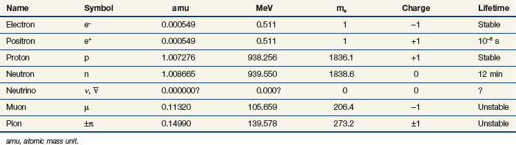
Particle mass can be expressed as the atomic mass unit (amu;  of the mass of the carbon nucleus) or in units of energy by conversion with Einstein’s formula, E = mc2. Table 6-2 gives the symbol, charge, mass, and stability for the electron, proton, neutron, and other particles of interest.
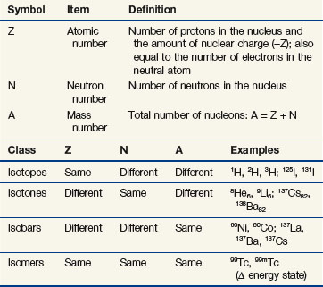
Combinations of nucleons form a variety of nuclei and determine the physical character of an atom. The number of protons in the nucleus, Z, is called the atomic number and determines the chemical properties of an atom and the atom’s identity as an element. The atomic number also equals the number of electrons in the neutral atom, with one electron per proton. The number of neutrons in the nucleus, N, is called the neutron number. Whole protons and neutrons constitute the nucleus, and Z and N have integer values. An atom’s mass number, A, is the sum of its neutrons and protons. The mass number (an integer) has a value close but not equal to the actual nuclear mass. Their values are similar but must not be confused. Nuclear mass is the noninteger sum of the masses of the individual particles minus their binding energies. Definitions for Z, N, and A are summarized in Table 6-3.
Nuclides and Radionuclides
Nuclides are atomic species made of different combinations of nucleons, and they may be classified by their number of protons, neutrons, or nucleons (Z, N, or A) and by their energy state. Nuclei with the same Z but different N are called isotopes (p for proton), and they exhibit identical chemical characteristics (they are the same elements). Nuclei with the same N but different Z are called isotones (n for neutron). Nuclei with the same A but different Z and N are called isobars. In a last category, nuclei with the same Z and N, and therefore A, but different nuclear energy states (i.e., excited vs. ground) are called isomers. Table 6-3 shows these classifications and example nuclides. A nuclide, or nuclear species, X, is denoted as


Not all combinations of Z and N exist in nature or can be manufactured. Instead, certain combinations are possible, whereas other combinations cannot occur. Figure 6-2 shows the distribution of stable nuclides as a function of the number of neutrons and protons. Notice that at low Z, the ratio of neutrons to protons (N : Z) is about 1.0. Above Z = 20, stable nuclides have more neutrons than protons (N : Z > 1.0). At higher Zs, the stability of nuclei tends toward neutron-rich nuclides. It has been observed that nuclei with 2, 8, 20, 28, 50, 82, or 126 nucleons (protons and neutrons combined) are stable. These stability “magic numbers” relate to the filling of nuclear energy levels, similar to the complete filling of electron shells. Pairing of like nucleons also results in increased nuclear stability. There are 165 stable nuclei with an even number of both protons and neutrons, 57 stable nuclei with an even number of protons and odd number of neutrons, 53 stable nuclei with an odd number of protons and even number of neutrons, but only 6 stable nuclei with an odd number of both protons and neutrons.
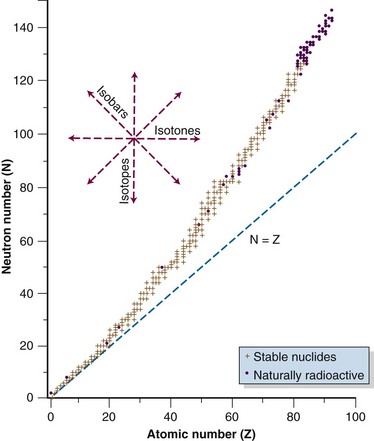
Figure 6-2 Distribution of stable and naturally radioactive nuclides.
Data from Radiological Health Handbook. Bethesda, Md., U.S. Department of Health, Education, and Welfare, 1970.
Some nuclides are unstable and eventually transform to stable states by the emission of particles or energy. These nuclides are called radionuclides or radioactive species, because a particle or energy is given off during the nuclear transition. Unstable nuclides lie off the line of stability and will have a neutron or proton excess relative to the stable nuclide. In Figure 6-2, isotopes lie along a vertical axis, isotones lie along a horizontal axis, and isobars lie at 45 degrees to either axis, perpendicular to the line of N = Z. Modes of radioactive decay depend on the type of nucleon excess, whether neutron or proton, and are discussed later in more detail.
Photons and Other Definitions
Interactions of ionizing radiation occur at the atomic and nuclear level, where binding energies are small compared with macroscopic realms. Electromagnetic radiation, or photons, are particles that have wavelike qualities with zero mass, which transfer energy from one location to another by propagation of an electromagnetic wave at the speed of light, c (c = 3 × 10⁸ m/s). Photons are also the mediators of charged particle bonds. A photon has wavelength λ, frequency ν, speed c = λν, and energy E = hν; c is the speed of light, and h is Planck’s constant (h = 6.626 × 10⁻³⁴ m2 kg/s). The electromagnetic spectrum consists of photons with wavelength, frequency, and energy ranges over 10 orders of magnitude (the range is really infinite). From low to high energy, there are radar waves, microwaves, infrared, light (visible photons), ultraviolet, x rays, and gamma rays. Photons are named by their wavelength (e.g., radar waves, microwaves), character (e.g., “purple”), and origins (e.g., x rays from the atom, gamma rays from the nucleus) (Table 6-4).
| Item | Symbol | Definition |
|---|---|---|
| Atom | a | Smallest subunit of an element retaining the character of that element; composed of a nucleus of protons and neutrons and orbital electrons |
| Electron | e− | Particle with a charge of −1 and mass of 0.511 MeV; used for radiation treatment when accelerated to energies capable of ionization |
| Photon | hν, γ, x | Particle with zero charge and mass consisting of electromagnetic radiation; used for radiation treatment at energies capable of ionizing matter |
| Gamma ray | γ | Photon (electromagnetic radiation) originating from within the nucleus as a result of nuclear transformations |
| X ray | x | Photon (electromagnetic radiation) originating from within the atom as a result of atomic transformations |
| Ionization | Removal of an electron from an atomic shell, leaving the atom with a charge of −1 | |
| Ionizing radiation | Radiation of sufficient energy to cause ionization upon interaction | |
| Ion | X−, X+ | Atom of element X with an electron deficit, as is formed after ionization, or an electron excess |
| Nonionizing radiation | Radiation of insufficient energy to cause ionization on interaction | |
| Electron volt | eV | The energy gained by 1 electron when it is accelerated through a potential of 1 V |
| Kiloelectron volts | keV | 1000 electron volts; used to denote the energy of a monoenergetic particle or photon, as in “100-keV photons” or “10-keV electrons” |
| Million electron volts | MeV | 1 million electron volts; used to denote the energy of a monoenergetic particle or photon, as in “1.17-MeV gamma rays” or “7-MeV electrons” (see Fig. 6-7) |
| Million volts | MV | Million volts; used to denote a spectrum of polyenergetic particles or photons with a maximum energy, as in “18-MV x rays.” In this example, the x rays have a maximum energy of 18 MeV and a continuous energy distribution of photons from 0 up to 18 MeV (see Fig. 6-7). |
Radiation Production and Treatment Machines
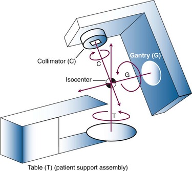
External beam radiation therapy machines produce ionizing radiation by (1) radioactive decay of a nuclide or (2) electronically by the acceleration of electrons or other charged particles such as protons. The basic purpose is to create an intense beam of ionizing radiation with known and predictable characteristics that can be aimed at a patient from a certain distance away (typically 80 to 100 cm). This beam of radiation with a source outside the patient is the “external beam.” The most commonly used radionuclide has been 60Co. Although once quite common as the first widely used device for external beam radiation therapy, 60Co treatment machines in the United States and other developed nations have been replaced over the past 20 to 30 years by linear accelerators, which produce high-energy x rays and electrons by electronic means. Basic components of all external beam treatment machines include a radiation source, a collimating system to form and direct a radiation beam, inherent or added shielding for radiation protection, a control system to turn the beam on and off, a light field to delineate visibly the radiation field to be treated, a means to rotate the beam or otherwise change its direction, and a support assembly for the patient. These components are assembled for modern conventional treatment machines in an isocentric geometry (Fig. 6-3). The isocenter is a point in space at which the treatment machine rotational axes all intersect. Any mechanical rotation is about an axis that passes through the isocenter. With many common components, 60Co teletherapy units and linear accelerators differ primarily in the method of photon production: radioactive source versus electronic source. In current configurations linear accelerators also offer a wide range of sophisticated control systems for control of radiation beam shape, intensity, and trajectory (discussed later).
Radiation Production by Radioactive Decay
Teletherapy is the use of radioactive material for production of an external beam of gamma rays for treatment at a distance from the radioactive source (tele, meaning “at a distance”). The term is historical and is in contrast to brachytherapy, where the radioactive source is placed in or on the treatment volume (brachy, meaning “close”). Gamma rays are emitted from a daughter nucleus formed after radioactive decay of an unstable parent nucleus. Each gamma ray has a unique energy that relates to the immediately preceding nuclear transformation, and this unique energy can be used to identify the daughter (and therefore the parent). 226Ra, 137Cs, and most commonly 60Co have been used for teletherapy. 137Cs and 60Co are manufactured and became available by neutron activation and as a by-product of fission after the invention of the nuclear reactor. Use of 60Co as a source of gamma rays for treatment was pioneered by H.E. Johns9 and represented a major step in obtaining high-energy photons above 1 MeV. At that time, electronic means of photon production from high-energy x-ray tubes was limited to 300 keV maximum because of electrical arcing at higher accelerating potentials. Particle accelerators were required to produce potentials above 300 keV (e.g., betatrons10 and van de Graaff accelerators11).
Although of historical interest for most readers, 60Co teletherapy units have lower cost and a relatively simple design with lower requirements for their operating environment compared with linear accelerators. For these reasons 60Co teletherapy devices are used worldwide in regions with limited resources for funding and operating infrastructure. A disadvantage is the constantly decreasing dose rate as a result of the decay of the 60Co source and the requirement for eventual replacement of the source. In a conventional 60Co teletherapy unit (Fig. 6-4), a cylindrical sealed-source capsule about 3 cm in diameter and 5 cm high contains pellets of 60Co. In each transformation a 60Co nucleus decays to 60Ni, with the prompt emission of two gamma rays at 1.17 and 1.33 MeV each (1.25 MeV average). Typical activity is 9000 Ci (3.33 × 10¹⁴ Bq) for a dose rate of approximately 3 Gy/min at 80 cm from the source (2 Gy/min at 100 cm from the source). The source decays with a half-life of 5.263 years and is replaced every 5 to 7 years when the dose rate becomes “too low.”
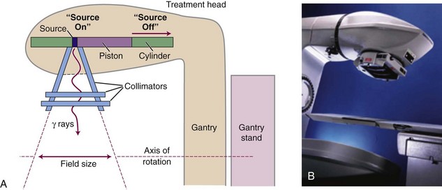
In one of the most commonly available teletherapy unit configurations (Theratron Phoenix, Best Theratronics Ltd, Ottawa, Ontario, Canada) the source is stored in a shielded head of the machine, mounted on the end of a movable piston in a horizontal cylinder (see Fig. 6-4). On the initiation of treatment, the source is moved pneumatically to a position over an opening in the shield that allows a treatment beam to exit. A collimator consisting of interleaved bars of a high Z material is used to define the field size as the beam exits the shield port. Trimmer bars can be used to reduce the beam penumbra, which is large because of the relatively large source size of approximately 1.5 inches. Maximum field size is 35 × 35 cm2 at 80 cm from the source. Irradiation time is measured and controlled by two independent timers. An end effect caused by the mechanical movement of the source, for which the effective irradiation time is less than the timer setting, is inherent and can be measured. Cross-hairs and a field light are used to delineate the central ray and field dimensions. There is a source-to-surface indicator. Source movement is designed so that in the event of treatment termination or device failure the source is automatically returned to the shielded condition. An emergency pushbar (T-bar) can be used to manually return the source to the shielded position, if necessary.
Radiation Production by Linear Accelerators
The principle of operation for linear accelerators is to accelerate electrons down a waveguide by use of alternating microwave fields.12 Two basic waveguide designs exist: standing wave and traveling wave. Waveguide length is a function of the maximum acceleration energy (longer is higher energy) and the frequency of the microwave field. The most common frequency for gantry-based linear accelerators (see later) is 2.998 GHz (S-band microwaves); however, specialized, shorter waveguides are possible at 9.3 GHz (X-band microwaves) that produce megavoltage energies above 6 MeV with acceptable dose rates for treatment. Major electronic components are described in Table 6-5 and are shown in Figure 6-5 for gantry-based linear accelerators, the most common design.
TABLE 6-5 Major Electronic Components of Linear Accelerators
| Component* | Purpose |
|---|---|
| Electron gun | Source of electrons to be accelerated |
| Microwave source | Provides accelerating potential and amplitude (power). Typically, magnetrons are used for ≤10 MV; klystrons are used for >10 MV and for most dual-energy machines. |
| Pulse-forming network | Synchronizes electron bunches with microwave phase |
| Transmission waveguide | Carries microwave power from its source to the accelerating waveguide |
| Injector | Injects pulses of current to the electron gun (i.e., drives electron gun) |
| Accelerating waveguide | Location of electron acceleration through multiple coupled cavities in a linear geometry (i.e., the linear accelerator) |
| Bending magnet | Used in horizontally oriented accelerating waveguides to redirect the electron beam, for electron energy selection, and for beam focusing |
| Target (for x rays) | Placed in electron beam for x ray production on electron impact |
| Scattering foils (for electrons) | Scatter electrons to produce a uniform beam of electrons for treatment |
| Flattening filter (for x rays) | Flattens the highly peaked x-ray beam exiting the target to produce a uniform beam of x rays for treatment |
| Monitor chambers | Ionization chambers that monitor the amount of radiation in the beam; count dose and turn machine off when set dose is reached; monitor beam flatness and symmetry |
| Collimators (secondary) | Provide rectangular field shaping for x rays and set field sizes for electrons |
| Accessories and beam modifiers† Interlocks† |
Define or modify beam shape or intensity With other control systems, ensure proper operation of linear accelerator for dose assurance and safety |
* Components are shown in Figure 6-5.
† Components are not shown in Figure 6-5.
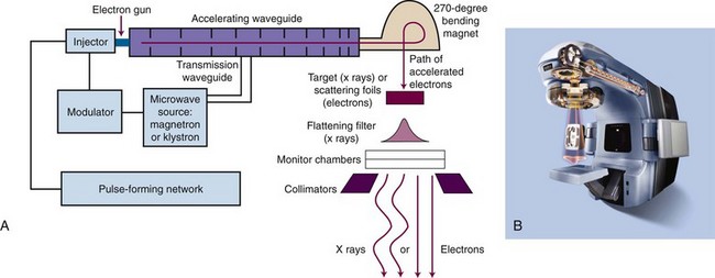
Major mechanical components are similar to those for teletherapy. A rigid, floor-mounted stand holds high voltage, microwave transport guides, cooling and control components, and supports a rotatable gantry holding the waveguide to allow 360-degree rotation of the source at an isocenter of 100 cm to enable multiple beam directions (see Fig. 6-3). In an alternative barrel-type design the entire accelerator—including waveguide, high voltage, microwave transport guides, and other components—is contained within a large rigid cylinder and the cylinder and all its contents rotate on a horizontal axis about the isocenter (this design not shown). A set of one or two pairs of high Z collimators (“jaws”), depending on the manufacturer’s design, provides at least 99.9% attenuation of the primary beam (0.1% transmission) and defines the length and/or width of the rectangular x-ray radiation field. A maximum field size of 40 × 40 cm2 at 100 cm (isocenter) is common, with 180-degree rotation of the entire collimator assembly about the isocenter. Collimator settings are continuously variable, and jaw pairs can be operated in coupled mode to produce symmetric, rectangular fields or, in most modern machines, independently to produce asymmetric fields. Asymmetric operation may include travel of one jaw across the central axis. Cross-hairs and a field light are used to delineate the central ray and field dimensions, and there is a source-to-surface indicator.
Although linear accelerators typically have had an isocentric rotating gantry, there are two other megavoltage accelerator designs available. One design, called tomotherapy, uses a highly stable CT-like ring gantry around which an X-band linear accelerator rotates, always pointed toward the rotational center (an isocenter).13 A binary (“on” or “off”) collimator intensity modulates a 6-MV x-ray fan beam as the accelerator waveguide is rotated. The treatment table is advanced in a stepwise or continuous motion for either slice-by-slice or helical fan beam treatment. Another approach uses a non-isocentric format with an X-band linear accelerator fixed on the end of a high-precision robot that is computer controlled for a range of motions with multiple degrees of freedom.14 This device produces a circular 6-MV x-ray beam that can be pointed at the target from various “nodes” in space—using a relatively large collection of irradiation nodes generates the cumulative dose distribution at the target.
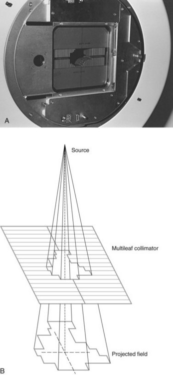
Accessories and beam modifiers for conventional geometry linear accelerators are important for customizing the external beam field to an individual patient and include custom or standard shielding blocks to shape a patient’s treatment fields to minimize the amount of normal tissue treated or protect critical structures; electron applicators for defining electron fields at the patient surface; physical and “virtual” or “dynamic” wedges for producing angled isodose distributions; and compensators for shaping the dose distribution within a patient for desired dose uniformity. Custom block manufacturing for shaping of patient-specific fields was once very common, using high Z alloy materials to provide primary beam attenuation of at least 97% (five half-valve layers [HVLs]). The use of custom blocks has been almost totally replaced by a versatile collimator design called the multileaf collimator (MLC), which is now available from all linear accelerator manufacturers (Fig. 6-6). The MLC provides field-shaping capabilities, replacing standard hand or custom blocks by the use of a large number of adjustable high Z vanes, or leaves. The desired beam outline is shaped as a series of steps by positioning each leaf to approximate a continuous field edge (see Fig. 6-6B). Different manufacturer’s MLC designs include singly and doubly focused leaf ends, where the leaf ends match beam divergence either across the direction of leaf travel (single) or both across and with the direction of leaf travel (double), and projected widths at the isocenter of 3 mm, 4 mm, 5 mm, or 10 mm.15 MLCs also have capabilities for dynamic treatment, as discussed later for intensity-modulated radiation therapy (IMRT).
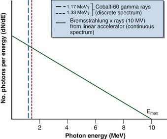
Three differences in radiation sources for teletherapy and linear accelerator devices are fundamental. First, a 60Co source is always “on” in that radioactive decay always occurs; the source must be moved to an unshielded condition to initiate an irradiation (see Fig. 6-4). With a linear accelerator, no source is present until the unit is energized; the irradiation is on or off with the flip of an electronic switch initiated by the operator with a key or button at the treatment console. Second, their photon spectra are different (Fig. 6-7). In a 60Co unit, two monoenergetic gamma rays are emitted with each decay to produce a discrete spectrum with peaks at 1.17 and 1.33 MeV. In contrast, a linear accelerator produces a continuous x-ray spectrum through the bremsstrahlung interaction. The spectrum has a maximum energy of Emax (i.e., accelerating potential) and all other photon energies down to zero. An average x-ray energy of approximately one-third Emax can be determined and is consistent with theoretical predictions for the continuous bremsstrahlung spectrum (see Fig. 6-7). Third, a linear accelerator can produce a treatment beam of electrons as well as photons. The accelerated electron beam is allowed to exit the machine under controlled conditions of scatter. Although 60Co gamma rays occur because of a priori beta decay, the beta particles (electrons) are stopped by the source capsule and cannot be otherwise harnessed for treatment.
Radiation Production by Other Accelerators
Other accelerator techniques have been used to produce a variety of high-energy particles such as electrons, protons, neutrons, and higher Z ions. These techniques include the betatron,10 van de Graaff accelerators,11 cyclotrons,16 the racetrack microtron,17 and accelerators18 used for high-energy physics experiments.
Among high-energy particles, protons have become the most attractive for therapeutic uses, where proton energies of 230 to 250 MeV yield treatment depths of up to 30 to 40 cm. Although currently a very expensive technology to build ($100 to $150 million) and maintain, the use of high-energy protons for treatment is increasing with 8 proton facilities in the United States and 33 sites worldwide (including a few for carbon ions).19 Typically, a fixed, single cyclotron has a beam line that is split to service one to four treatment rooms, each with a movable gantry to aim the proton beam. Alternative designs include the use of a smaller (though still large) cyclotron that is mounted on a very large double-legged gantry system that enables rotation about the patient, and a new novel design that uses the principle of dielectric wall acceleration in a relatively compact device (2.0 to 2.5 m length) that would potentially fit within a standard-size treatment room. Facility designs and technical aspects for proton therapy have been discussed.20
Interactions of Ionizing Radiation with Matter
Photon Interactions
Attenuation and Transmission
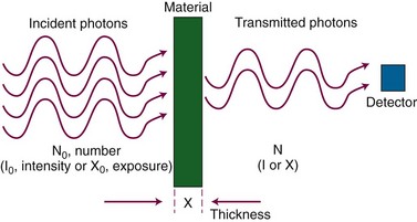
When incident on matter, ionizing photon radiation undergoes interactions with atomic electrons or nuclei. Interacting photons are removed from the primary beam, an effect called attenuation. Photons that do not interact and instead exit the material are called transmitted photons. Attenuation and transmission are illustrated in Figure 6-8. A number, N0, of monoenergetic x rays or gamma rays is incident to a slab of material, and a smaller number, N, is transmitted. The attenuated photons, N0 and N, are absorbed in the material or scattered in other directions. In narrow-beam geometry, N transmitted photons alone reach a detector as shown. In broad-beam geometry, scattered photons also reach the detector.
Constant fractional attenuation per unit thickness compounds over successive thicknesses, illustrated in Figure 6-9. This “fraction of a fraction” effect is nonlinear, and the integrated form of Equation 1 yields an important relationship: attenuation in a continuous material is an exponential process:
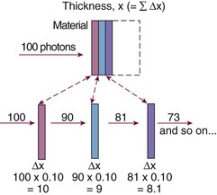
In Equation 2, N0 is the original number of incident photons, N(x) is the transmitted (unattenuated) number of photons, e is Euler’s constant (e ≈ 2.7), µ is the linear attenuation coefficient, and x is the thickness traversed by the photons.
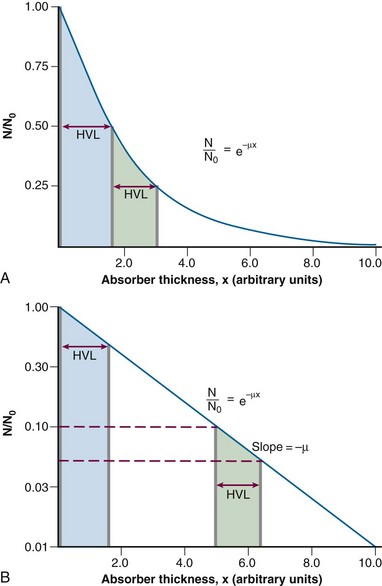
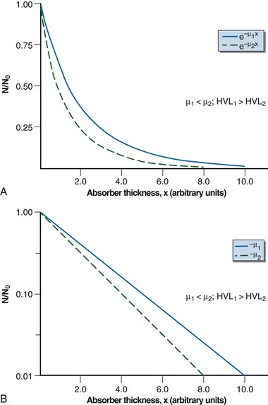
Equation 2 can be graphed in linear or semi-log form (Fig. 6-10). In semi-log form, the attenuation curve is a straight line with a slope of −µ (see Fig. 6-10B). A smaller attenuation coefficient means less attenuation and a shallower attenuation curve. Different attenuation coefficients result in a different amount of attenuation for the same thickness traversed and attenuation curves that differ in their slopes (Fig. 6-11). A smaller attenuation coefficient results in less attenuation.
Beam Quality
 , the thickness, x, is the HVL, and the attenuation equation becomes
Two important relationships come from this equation:

 , and given a thickness of material in units of HVL (x = n HVL), the amount of attenuation can be computed by
In Equation 5, I/I0 is the fractional transmission, intensity, or exposure and n is the thickness of the material in number of HVLs.
In Equation 6, m is the thickness of the material given in number of TVLs.
HVL can be found graphically from the attenuation curve, whether on a linear or log plot (see Fig. 6-10) and for monoenergetic photons can be determined anywhere along the curve because µ is constant; the ratio of the two intensities must be  . For polyenergetic photons, µ is not constant but instead decreases with increasing depth (Fig. 6-12A). The low-energy component of the beam spectrum is attenuated preferentially, compared with high-energy photons, because of increased attenuation at low energies. As depth increases, the ratio of high-energy to low-energy photons increases, resulting in increased beam penetration, or “beam hardening.” After a large number of low-energy photons are attenuated at depth, beam hardening is minimal and µ is essentially constant. The log attenuation curve begins steeply, has curvature, and then becomes linear at depth (see Fig. 6-12B). Because µ changes with depth, HVL also changes, yielding different first and second HVLs, as defined in Figure 6-12B. The monoenergetic case is shown for comparison. HVL1 is always less than HVL2 because photons incident on HVL2 have a higher average energy:
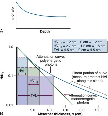
Characteristics of attenuation curves for monoenergetic and polyenergetic photons are summarized in Table 6-6.
| Monoenergetic | Polyenergetic |
|---|---|
| 1.Exponential curve on linear paper | 1.Complex exponential curve on linear paper |
| 2.Linear curve on semi-log paper | 2.Curved on semi-log paper |
| 3.Constant µ | 3.Varying µ:µeff can be determined |
| 4.Constant HVL | 4.Varying HVL: HVL1, HVL2, TVL, and greatest HVL can be determined |
HVL, half-value layer; TVL, tenth-value layer. See text for other terms.
Attenuation Coefficients

Attenuation coefficients can also be expressed in other forms and can be converted from one form to another.21
Photon Interactions: X Rays and Gamma Rays


In the previous equations, TOT signifies the total coefficient and COH, PE, CE, PP, and PD refer to the respective five interactions. The photoelectric effect, Compton effect, and pair production are the most important interactions for megavoltage photons used for radiotherapy. Detailed presentations of these five interactions have been published.2,21,22
Coherent Scattering
In coherent scattering, a photon is scattered off an outer orbital electron with a change in direction and no change in energy (Fig. 6-13). At very low energies (<10 keV), the amount of coherent scattering can be large and attenuation can be high, even though there is no change in photon energy. The amount of coherent scattering is negligible in the diagnostic and therapy energy ranges compared with other principal interactions.
Photoelectric Effect
The following actions occur in the photoelectric effect (Fig. 6-14):
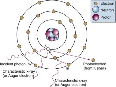
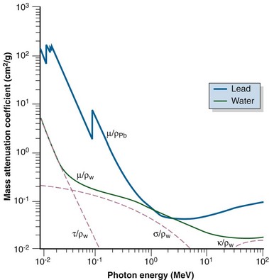
The photoelectric effect has a strong dependency on photon energy and atomic number of the material. The mass attenuation coefficient varies as (1/Eγ)3 and Z3, respectively. Mathematically, this is shown as follows, where CPE is a proportionality constant:
These dependencies for water are shown graphically in Figure 6-16. In the photoelectric effect, no interaction is possible until the photon energy is greater than the electron binding energy. After the binding energy is barely exceeded, the probability for interaction increases greatly, leading to a sharp increase in µ/ρPE, called an absorption edge. In Figure 6-16, the K and L edge for lead are seen, corresponding to photoelectric interactions for the K and L shell electrons. No absorption edges are shown for water; the binding energies are less than 1 keV and do not show up on the plot.
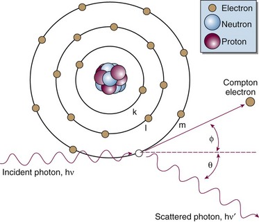
Compton Effect
In the Compton effect (see Fig. 6-15), several things occur:
In Equation 12, α = hν/moc2 and represents the ratio of the incident photon energy to the rest mass of the electron, mo, and θ is the angle of photon scattering as defined in Figure 6-15.
The Compton electron has energy Ece given by the following equation:
and a scattering angle, φ, that depends on the incident photon’s energy and its scattering angle, θ:
A few scattering cases can be considered:
 moc2) even as the incident photon energy becomes very large. The electron has maximum energy of Ece = hν − hν′ = hν (2α/(1 + 2α)) and travels in the forward direction.
Although isotopically distributed for lower-energy photons, Compton electrons scatter more and more in the forward direction as incident photon energy increases. Their average energy also increases from about 10 keV to 7 MeV as incident photon energy increases from about 100 keV to 10 MeV.11 The forward-peaked distribution is responsible for the buildup region for megavoltage photon beams, as explained later.
The Compton effect has a slight dependency on incident photon energy, decreasing as energy increases through the megavoltage range, but the interaction probability is essentially constant over most of the megavoltage energy range (see Fig. 6-16). Compton scattering is independent of atomic number and is dependent on the number of electrons available, or electron density (electrons per gram). The electron density for almost all materials is constant at approximately 3 × 10²³ electrons per gram because N : Z is almost constant. The exception is hydrogen, which with one proton in the nucleus has an electron density of around 6 × 10²³ electrons per gram. Except for a small energy dependency and increased interaction probabilities for hydrogen-laden materials, the Compton mass attenuation coefficient is remarkably constant across energy and atomic number, especially for low Z biologic materials such as tissues. Mathematically, this relationship is
In Equation 17, CCE is almost a constant.
Attenuation by the Compton effect reduces to the following expression:
Pair Production
In pair production (Fig. 6-17), the following steps occur:
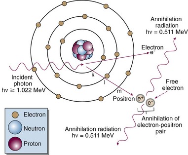
The electron and positron travel off in no particular directions and do not have equal energies.
Distribution of Secondary Electrons
Electrons released by ionizing photon interactions can travel in any direction from the interaction point and in general have a complex probability for angular spread, depending on incident photon energy and the interaction that occurs. The probability for forward directions increases with photon energy and is a likely direction for megavoltage photon interactions.2 As seen later, angular scattering of electrons is responsible for a number of characteristics for megavoltage photon beams, including surface dose, the buildup region, the depth of maximum dose, and the penumbra region.
Total Attenuation Coefficient
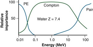
In Figure 6-16, the individual interaction and total mass attenuation coefficients are shown as a function of energy for lead and water. Notice the K edge in the curve for lead. It can be seen that different energy regions are dominated by particular interactions. For water, the photoelectric effect dominates for photon energies up to 60 keV, the Compton dominates from 60 keV to 10 MeV, and pair production dominates approximately above 10 MeV. For lead, the photoelectric effect dominates up to 700 keV, the Compton effect from 700 keV to 3 MeV, and pair production at 3 MeV and higher. An interaction’s region of dominance can be represented graphically to show relative importance as a function of energy (Fig. 6-19).
Comparison of interaction dependencies shows why diagnostic energy photons give good contrast for imaging: the photoelectric effect dominates and is quite sensitive to the atomic numbers of the materials being imaged. Materials with even slightly different Zs have good subject contrast (and image contrast) because attenuation depends on the cube of the atomic numbers. Radiotherapy port films, however, have poor contrast because the dominant interaction is the Compton effect. There is no dependence on atomic number, and the effect is constant for most biologic materials (except for hydrogenous materials). Instead of imaging atomic number, the Compton effect images the density of a material, and subject contrast is essentially density differences. A comparison of simulator and port films is given later (see Fig. 6-49).
Total Absorption Coefficient
Radiation dose relates directly to the amount of energy absorbed at a point, not the amount attenuated, although the two are intimately related. This transfer of energy is done by secondary electrons (photoelectrons, Compton electrons, and the electron-positron pair) that produce ionizations along their paths until their energy is expended. A portion of the photon energy that is attenuated may escape to other regions as a coherent or Compton scattered photon, an annihilation photon (0.511 MeV), or a bremsstrahlung photon after radiative collision of a secondary electron. The amount of energy absorbed from secondary electrons is less than the amount attenuated as photons, as described by Johns.21 In a similar fashion to the total mass attenuation coefficient, the total mass energy absorption coefficient, µen/ρ, or simply the mass absorption coefficient, describes the energy absorbed due to each interaction and is used for computing dose. The value of µen/ρ is first equal to µTOT/ρ in the photoelectric region (because all photon energy is transferred to the photoelectron), and then µen/ρ is less than µTOT/ρ in the region where the Compton effect dominates (because the Compton scattered photon carries energy away). At very high energies where pair production dominates, µen/ρ and µTOT/ρ are almost equal because the fraction of incident photon energy carried off as annihilation photons is negligible compared with the amount transferred to kinetic energy of the electron-positron pair. Over the energy range used for radiotherapy, the amount of absorbed energy at a point in water (tissue) is about one half the amount attenuated at the point. The mass absorption coefficient and dose are discussed more in the next section.
Summary of Photon Interactions
Charged Particle Interactions
Charged particles incident on matter undergo inelastic and elastic interactions with atomic electrons and nuclei, that is, other charged entities.2,12,13 Inelastic interactions include collisional and radiative processes and result in energy loss by the particle. In an elastic interaction the particle is scattered by an atomic electron or nucleus, resulting in a change of direction for the particle but no energy loss. The interaction probability for charged particles is effectively 1; an incident particle interacts at every opportunity. The quotient dE/dx (units of million electron volts per centimeter) is called the stopping power, and it describes the rate of energy loss, dE, that occurs over distance traveled, dx, for inelastic collisions. Stopping power is often expressed as the mass stopping power, dE/ρdx (units of million electron volts per gram per square centimeter), which is independent of the absorber density. Because energy loss is almost continuous and a particle has a particular kinetic energy, EKE, the particle loses this amount of energy and then stops. The distance traveled is finite and is called the particle range; the particle can go no farther, and its kinetic energy is zero. For an absorber of density ρ, the particle range, r, can be calculated as follows:
In Equation 21, z is the atomic number of the incident particle of mass M, V is its velocity, e is the electron charge, mo is the electron mass, NZ is the number of electrons per cubic centimeter in the absorber, and FQ is a complex function describing energy transfer per interaction.
Collisional energy losses increase by the square of the particle’s atomic number and as the incident particle velocity decreases. Increased atomic number results in a greater coulomb force, and decreased velocity increases the amount of interaction time, both leading to increased dE/dx. The energy transfer function, FQ, is complex and varies with the type of interaction.2 It accounts for the atomic mass of the absorber, ionization potential, and relativistic effects as V approaches the speed of light.
Light Charged Particle Interactions: Electrons
The electron mass is small compared with any atomic mass, and incident electrons undergo four types of particle interactions with a large amount of scattering.8 Collisional interactions result in energy loss of dECOL/dx, causing ionizations or excited states (higher electron orbits) (Fig. 6-20). Collisional losses increase as the electron velocity decreases, as stated earlier, and decrease as the absorber atomic number increases. The decrease with absorber atomic number results from the decrease in the number of electrons per gram (NZ/ρ) as Z increases. For equivalent mass thicknesses (mass thickness is thickness divided by density, with units of square centimeters per gram), electrons are stopped sooner in low Z than in high Z materials. Figure 6-21 shows these relationships for water and lead.
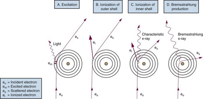
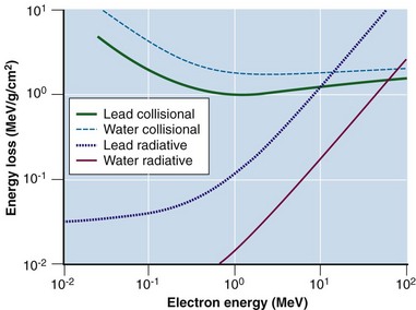
Figure 6-21 Collisional and radiative electron losses as a function of incident electron energy.
Adapted from Johns HE, Cunningham JR: The Physics of Radiology, ed 3, Springfield, Ill., 1978, Charles C Thomas.
Radiative interactions result in x-ray emissions. The incident electron penetrates the electron cloud and interacts with the nucleus’s positive electrical field, undergoing an abrupt deceleration with energy loss dERAD/dx and a change in direction (see Fig. 6-20D). The energy change, dERAD/dx, is released in the form of x rays, called bremsstrahlung (or braking) radiation. With an incident monoenergetic electron fluence, a continuous x ray spectrum is emitted because the probability of any energy loss, large or small, is equal per interaction. Successive bremsstrahlung interactions may occur as the electron loses its energy; a bremsstrahlung spectrum has a maximum energy equal to the initial electron energy and energies below to zero (see Fig. 6-7). Radiative interactions are important; they are the mechanism by which bremsstrahlung x rays are produced in diagnostic x-ray tubes and linear accelerators. Bremsstrahlung production increases with incident electron energy and the Z of the absorber (see Fig. 6-21).
The probability for collisional and radiative interactions depends on electron energy and the atomic number of the incident material (see Fig. 6-21). At electron energies of 100 keV and for high Z absorbers (e.g., x-ray targets), 99% of the interactions are collisional and 1% are radiative, resulting ultimately in heat deposition. At electron energies of 10 MeV, bremsstrahlung is a much more efficient process, and 50% of the interactions are collisional and 50% radiative. At 100 keV, x ray production is inefficient, whereas at 10 MeV, x ray production is efficient. Above 10 MeV, bremsstrahlung production exceeds collisional losses. It has been observed that dECOL/dx increases as electron kinetic energy decreases below 1 MeV (see Fig. 6-21). As the electron slows down, it loses energy faster. Above 1 MeV, electrons lose about 2 MeV/cm traveling in water (dECOL/dx ≈ 2 MeV/cm). A 10-MeV electron has a range of about 5 cm in water (10 MeV ÷ 2 MeV/cm). Density scaling can be applied for materials different from unit density. For example, a 10-MeV electron travels approximately 3.3 cm in bone of density of 1.5 g/cm3 (10 MeV ÷ [2 MeV/cm × 1.5]). These relationships use Equation 20 as their basis.
Heavy Charged Particle Interactions
Heavy charged particles, such as protons and alpha particles, experience mainly inelastic collisions. The rate of energy loss is high, resulting in short ranges. Trajectories in water or tissue are in the forward direction with little scattering; the particle mass is similar to that of the interacting material, and very few large-angle direction changes occur, in contrast to the large amount of scattering experienced by electrons. Heavy charged particles exhibit rapidly increasing and large energy losses near the end of their ranges, because of the dependency on Z2 and 1/V2 discussed earlier (see Eq. 21). This increase in energy loss results in a dramatic increase in ionization at the tail of the particle track length after a length of relatively constant loss, a phenomenon called the Bragg peak.2,12,13 Bragg peaks are observable for protons (Fig. 6-22) and alpha particles. All charged particles exhibit a Bragg peak, including electrons; however, electrons are light enough such that multiple scatters occur and ionization paths are randomly oriented, blurring any observable effect.
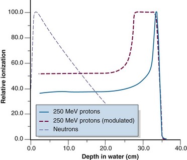
The proton finite range can be modulated through a physical attenuator to decrease the range from the maximum. If range modulation is done continuously while the beam is on, the Bragg peak will be swept over a range and produce a high dose plateau (see Fig. 6-22). The width of the dose plateau can be designed to match a tumor size at a certain depth and demonstrates the attractiveness of protons for radiotherapy.
Heavy Uncharged Particle Interactions: the Neutron
Neutrons have no charge and do not undergo coulomb interactions like charged particles. Instead, neutrons interact by inelastic and elastic collisions with nuclei through the strong force. Commonly for lower and middle Z materials, a neutron penetrates the nucleus and is absorbed, followed by the ejection of a proton (the [n, p] reaction). The new nucleus may be radioactive, a process called neutron activation. Neutrons may also cause nuclear disintegrations, similar to photodisintegration. For very heavy nuclei, neutrons may cause fission, a reaction harnessed for power production in nuclear reactors. Elastic scattering of neutrons is also common. The type of collision, inelastic or elastic, that a neutron experiences depends on the neutron energy and the absorber atomic number with complex reaction probabilities.18,21 Neutrons lack charge, thus their interactions with nuclei are exponential in nature, like photons (see Fig. 6-22). Their range can be stated as a mean path length equal to the inverse of the neutron attenuation coefficient.
Summary of Particle Interactions
Radiation Quantities and Measurement
Ionization and Its Fate
Ionizing radiation is quantified by measuring the amount of ionization produced. The number of ions is directly proportional to the amount of energy imparted to a material. An average of 33.92 eV is required to produce one ion pair (ip) in air.23 This number is called the W value (W = 33.92 eV/ip for air), and it is almost independent of the radiation energy. W for other gases is quite similar to that of air, and its uniformity from material to material relates to atomic energy levels and capabilities for transfer of excitation energy.2
If these ions are collected and measured, the amount of energy deposited can be determined.
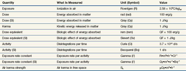
Radiation Quantities and Units
Exposure

Several important concepts characterize the roentgen:
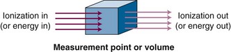
Electronic Equilibrium
With electronic equilibrium, ionization lost downstream from a volume of interest is replaced by an equal amount from upstream, producing an equilibrium and an accurate ionization measurement. The concept is illustrated in Figure 6-23. After interaction, ionization (electrons) travels away from the interaction point in the direction of the incident photons and a portion actually leaves the volume. To accurately measure the amount of ionization produced, the lost kinetic energy of the escaping electrons must be replaced by an equal amount that enters the volume from upstream (see Fig. 6-23). This equilibrium is called electronic equilibrium or charged-particle equilibrium and is a required condition for measurement of exposure.
Dose
Dose, D, is the measurement of the amount of energy imparted per mass of material (energy per mass).11 The unit of dose is the gray (Gy): 1 Gy = 1 J/kg. An earlier dose unit is the rad (rad): 1 rad = 100 erg/g = 0.01 Gy = 1 cGy; 1 Gy = 100 rad.
Dose does not have the restrictions of exposure, and the following two statements therefore apply:
In practice, dose to a medium is determined by measuring exposure and converting it to dose using the W value and the mass energy absorption coefficient, µen/ρ. The mass energy absorption coefficient is similar to the mass attenuation coefficient, except it describes energy absorbed, not attenuated. The process is illustrated in Figure 6-24 for the following steps:
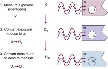
Figure 6-24 The dose measurement process. Exposure to a small mass of air is converted to the dose to medium.


For X number of roentgens, the dose to air is calculated as follows:

is the mass energy absorption coefficient for the material,


Combining Equations 23 and 24 yields the following expressions:

in which the f factor, f, is calculated as follows:
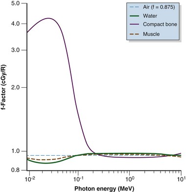
The f factor is an important parameter, and it varies as a function of the material and the photon energy, as shown for water, muscle, and bone in Figure 6-25. By its definition, the f factor for air is always 0.875. Water, muscle, and air have similar f factors because their effective atomic numbers are similar. Bone has a higher atomic number (by a factor of 2) and receives up to four times the dose that soft tissue would receive in the photoelectric region. This effect is responsible for high bone doses received during orthovoltage treatment as well as the contrast seen in diagnostic x-ray images. Notice the decrease in the f factor for fat in the photoelectric region because of its lower Z as a result of its high hydrogen content.
Kerma
Thorough treatments of exposure, dose, kerma, and their relationships are available.12,13,14 Much has been studied and written about these and other dosimetric concepts to establish meaningful and consistent definitions. A summary is presented in Table 6-7.
Radiation Detection and Measurement
Gas-Filled Detectors
Gas-filled detectors operate on the basic principle of measuring exposure, that is, collecting ionization in air or a substitute gas. A gas-filled volume is defined as one that contains two oppositely charged plates or wires to collect the charge resulting from ionization in the gas. The reading is in units of charge (coulombs), exposure, or exposure rate. Figure 6-26A shows a simple parallel plate gas-filled detector and its components. As the voltage applied to the electrodes is increased from zero, the amount of charge collected increases (see Fig. 6-26B). The distinct voltage regions are expanded in Table 6-8. In general, gas-filled detectors require calibration before making radiation measurements.
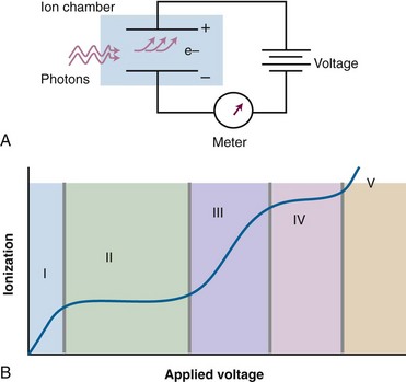
| Region | Description |
|---|---|
| I | The recombination region. The voltage is not high enough to separate the ion pairs and recombination occurs. |
| II | The saturation region. The voltage is high enough to collect almost 100% of the ionization (hence, “saturation”). Also called the ionization region. |
| III | The proportional, or gas amplification, region. The voltage is high enough to accelerate the ionized electrons to an energy that causes additional ionization, amplifying the actual amount of initial ionization by a factor M. |
| IV | The Geiger-Muller, or GM, region. The voltage is high enough that amplification by accelerated ions proceeds so that the entire gas in the detector is ionized each time a photon hits the detector. Whether low or high energy, the amount of ionization that occurs is the same. Thus, a GM counter emits a “click” for each photon seen and is really a photon counting device. |
| V | The continuous discharge region. The voltage is high enough to spontaneously ionize the detector gas. Once started, the ionization continues and continues. The detector is not useful at this applied voltage. |
Ionization Chambers
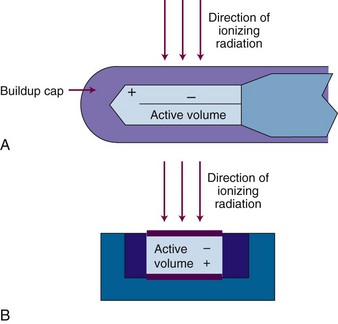
Ionization chambers operate in region II (see Fig. 6-26B) and are an important type of radiation dosimeter as the principal device used for calibration of radiotherapy beams. The design most commonly used for photon beams is the thimble chamber, also called a Farmer chamber, which has a cylindrical geometry with central linear and outer cylindrical electrodes (Fig. 6-27A). An active volume of 0.6 cc is convention, although chambers with smaller or larger volumes are available for specialized purposes such as small field dosimetry or low-dose-rate measurements. Parallel-plate chambers are also used and are the recommended chamber geometry for electron beam dosimetry (see Fig. 6-27B). In general, ionization chambers require calibration before use. Ionization currents produced by radiation beams are very small, on the order of 10−9 amperes (A), and require a high-precision device called an electrometer for accurate measurement. An ionization chamber and electrometer require calibration before use and with a triaxial connecting cable are required tools for radiation beam calibration. Conditions for radiation beam calibrations are set by national protocols such as the Task Group (TG)-51 from the American Association of Physicists in Medicine15 and by national or state regulatory bodies. A requirement for operation of all ionization chambers is that the chamber be operated under conditions of electronic equilibrium. In disequilibrium conditions, the amount of ionization measured is incorrect, as will be the exposure or dose calculation.
Solid-State Detectors
Thermoluminescent Dosimeters
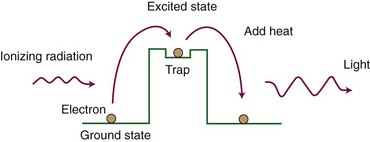
In a simple model, crystalline solids have two electron energy levels, called the valence and conduction bands. The valence band holds bound electrons, whereas the conduction band consists of free electrons. Energy states between these two bands are forbidden. When ionized, a bound electron may gain sufficient energy to jump to the conduction band, leaving a positive “hole” in the valence band. The conduction band electron and the hole can move through the lattice and eventually recombine, with the emission of light on recombination. Because of impurities in the lattice, some crystalline materials have the property of having long-lived “traps” that can hold an electron-hole pair in an excited (or unfilled) state. The electron-hole pair is created and excited into the trap by the absorption of ionizing radiation, which provides the energy to push the pair into the trap (Fig. 6-28). Heating the crystal enables the electron-hole pair to leave the trap and return to the de-excited state. With this transition, an amount of light is emitted that is proportional to the amount of radiation dose. Dose is measured by measuring the amount of light emitted. The two most common types of thermoluminescent dosimeter (TLD) are lithium fluoride (LiF, almost tissue equivalent) and calcium fluoride (CaF, not tissue equivalent). A calibration factor must be obtained before use as a dosimeter. TLD is used for in vivo patient dose monitoring during treatment and for personnel monitoring for radiation safety purposes.
Film
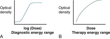
Film is a solid-state detector and typically refers to silver-halide films that are sensitive to both light and ionizing radiation. The amount of optical density is proportional to the dose. The response is energy sensitive because film is relatively high Z (the silver content). Response curves are shown in Figure 6-29. Film is used to obtain relative dose distributions (i.e., isodose distributions) for treatment machine quality assurance tests for flatness, symmetry, radiation/light field congruence, and imaging.16,25 A dose-response curve must be carefully measured, including constant processor control, to enable film to be used to measure actual (not relative) doses. Because of digital image receptors for photography and medical imaging with kV and MV photons (e.g., diagnosis and treatment verification), relatively high cost, and the development process required after exposure, medical uses of silver-halide radiographic film are almost nonexistent. For physics quality assurance and dosimetry purposes a new type of tissue-equivalent film, called radiochromic film, has become a powerful tool. Radiochromic film uses opacity changes from radiation-induced polymerization to indicate dose.26 This film does not require developing but does have an optimal wavelength of light for reading. A digital flatbed three-channel (color) scanner can be used to read the radiochromic film opacity. Example uses in therapy beam quality assurance and dosimetry include small beam dosimetry, patient treatment plan verification (such as currently performed prior to a first IMRT procedure), and mechanical and radiologic quality assurance in radiosurgery. Radiochromic film is tissue equivalent and can be used over the full range of x-ray energies. Radiochromic film types are also available for different dose ranges, from 1 Gy up to 50 Gy. Currently, radiochromic film is not an acceptable medical imaging device because of its cost and lack of imaging contrast.
MOSFET Detectors
A semiconductor device called the metal oxide-silicon semiconductor field effect transistor, or MOSFET, can be used as a radiation detector for in vivo dosimetry and physics quality assurance. The p-type device generates electron-hole pairs during irradiation proportional to the dose delivered, and the number of holes, corresponding to dose, can later be read using an appropriate metering device. Advantages include very small size, which enables small field or “point” dose measurements, and the capability for being incorporated into both implantable dosimeters and surface-placed dosimeters for in vivo patient dosimetry.27 MOSFET dosimeters are primarily used for photons and require calibration for the photon energy in use. Surface applications require an understanding of the build-up effect for proper assessment of surface dose.
Scintillation Detectors
Scintillation (light) detectors detect radiation by measuring the amount of light produced in special crystalline materials by the ionizing radiation. The most common material used is sodium iodine (NaI). The NaI crystal is coupled to a photomultiplier tube that amplifies the detection signal coming from the crystal (Fig. 6-30A). NaI detectors are extremely sensitive and detect background radiation easily. They are used to detect low-energy or low-activity (dose rate) sources. They are used in uncalibrated form; a pulse indicates a photon has been detected.
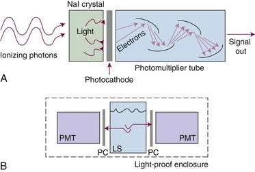
Scintillation materials can also be made in liquid form. With this technique a radiation source (i.e., a sample of radioactive material) is put in direct contact with a liquid scintillator by immersion (see Fig. 6-30B). This intimate contact enables extremely small activities to be detected. Detection limits are in the microcurie and picocurie ranges. This method is used most for detection of very-low-energy beta particles for radioisotope tracer studies, environmental sampling, and isotope analysis of waste or other materials. The liquid scintillator is called a cocktail and includes a solvent and the scintillation material. Liquid scintillation detectors require calibration before use, including determination of background count rates.
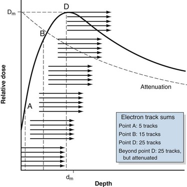
Buildup Phenomenon
Megavoltage photon beams used for radiotherapy exhibit a phenomenon in which the dose in an absorber is relatively low at the surface but rapidly increases to a maximum during the next few millimeters or tens of millimeters. This region of rapidly increasing dose is called the buildup region and is explained as follows. The secondary electrons produced by megavoltage photon interactions travel primarily in the forward direction from the interaction point. The direction and range are represented by the groups of arrows in Figure 6-31. The surface is the first point of interaction, and the dose from these interactions is delivered in the forward direction (point A). Because there are no interaction points upstream from the surface to produce secondary electrons, the surface dose is low. Ignoring attenuation and other small changes to the photon fluence with depth, interactions occur in the next layer of material beneath the surface, with a similar forward dose distribution. These electron tracks overlap (sum) with those from the surface. Additional layers at depth have similar interactions and resulting secondary electron distributions that sum with previous ones. The amount of dose increases rapidly and nonlinearly as successive electron tracks overlap (point B). Given an average, finite secondary electron range, a point is eventually reached where full electron overlap occurs (point D). At this point, the number of summed electron tracks is constant because the electrons being produced match those being lost. A maximum dose, Dm, is reached at a depth called dm (see Fig. 6-31), and dm indicates the average secondary electron range and is the point at which electronic equilibrium is obtained. Because photon attenuation occurs, the number of interactions and resulting secondary electrons decreases with depth from the surface. Attenuation competes with the buildup process; however, buildup is more rapid than attenuation, resulting in a net gain of dose. The presence and steepness of a buildup region depend on incident photon energy that governs the type of interaction and the range and distribution of secondary electrons. At higher photon energies, dm is larger because the average secondary electron range is greater. Beyond dm, photon attenuation results in transient electronic equilibrium (i.e., energy in is slightly greater than energy out) and a decrease in dose with depth (shown in Fig. 6-31 as the dotted line; the difference is exaggerated).
Dose Relationships for External Beams
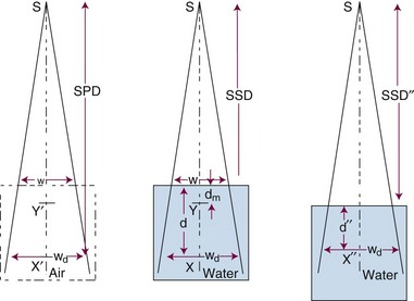
Three mathematical functions are used to describe the dose characteristics for external radiation beams: percent depth dose (PDD), tissue-air ratio (TAR), and tissue-phantom ratio (TPR).12,13 These dose functions relate the dose at any point to the dose at a reference point. The irradiation geometry shown in Figure 6-32 illustrates the measurement conditions for the following discussions.29
Percent Depth Dose
The PDD is the ratio of the dose at depth, Dd, to the maximum dose, Dm, measured along the central axis of the beam and expressed as a percent. Points X and Y are the locations at depth, Dd and Dm, respectively, in Figure 6-32B. PDD is dependent on the depth, d, reference depth, dm (the point of maximum dose), beam quality (or energy), E, source-to-surface distance, SSD, and field size at the surface, w. Mathematically,
Tissue-Air Ratio
Given a fixed irradiation point in space, the ratio of the dose in phantom, Dx, to the dose in air, Dx′, at the same point is called the TAR (see Fig. 6-32A and B). TAR indicates how the dose in air is affected when the air is replaced by tissue. The field size at the point and source-to-point distance are constant; the only variable is the depth in phantom:
Tissue-Phantom Ratio
TPR must be used for photon energies above about 4 MV, when in-air measurements required for the TAR are impractical. As with PDD and the TAR, the TPR is the ratio of two doses; however, both doses are made in phantom. The TPR is the ratio of dose Dx, measured at depth d, to dose Dx″, measured at a reference depth d″ (see Fig. 6-32B and C):
Primary and Scatter Dose: The Scatter-Air Ratio
Mayneord first proposed that PDD could be separated into primary and secondary (or scatter) components.12 Later, Clarkson30 proposed sector integration of scatter components in calculating the PDD at any point inside or outside an irregular field. This concept was later applied by Gupta and Cunningham to the TAR.31 The concept states that dose at a point is the sum of primary and scatter components. The primary dose results from photons that have interactions at the point of interest. The secondary dose results from photons and electrons that scatter to the point of interest from other interaction points. With this concept, TAR is given by the following expression:


The irregular field SAR is found by sector integration:
Although PDD can be measured with an ionization chamber beyond dm over the wide range of clinically used photon energies, the TAR cannot be measured when the photon energy exceeds about 3 MV because the range of secondary electrons exceeds the thickness of the buildup cap for the ionization chamber. At these energies, PDD is measured and converted to TPR and TMR by well-known relationships.21,22 PDD remains the most important and fundamental dose function and performance specification to be measured for almost all physics quality assurance procedures for all external beam treatment devices.
Characteristics of Radiotherapy Photon Beams
Dose Characteristics
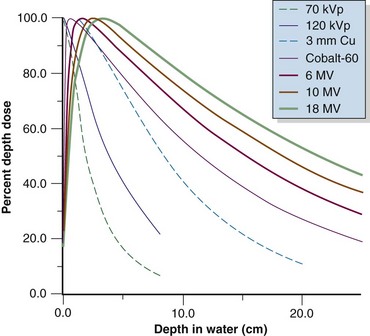
Photon beams used in radiotherapy have dose characteristics that vary primarily as a function of beam energy and treatment machine design. In the standard irradiation geometry (see Fig. 6-32B and C), PDD measurements are obtained in water along the central axis, beginning at the surface and proceeding to depth. A typical PDD curve shown in Figure 6-33 for megavoltage beams has the characteristics listed in Table 6-9.
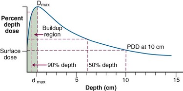
TABLE 6-9 Characteristics of a Typical Percent Depth Dose Curve for Megavoltage Beams
| Characteristic | Definition |
|---|---|
| Surface dose | Nonzero dose at the incident surface |
| Buildup region | Region between the incident surface and dmax where the dose rapidly increase |
| Dmax | Maximum dose along the central axis; often used as a reference dose |
| dmax | Depth of maximum dose; often used as a reference point |
| Percent depth dose | Dose along the central axis of the beam, as a percentage of the dmax dose |
| 90% dose depth | Depth from the surface where the dose in the buildup region reaches 90% of Dmax |
| 50% dose depth | Depth from the surface beyond dmax, where the dose falls to 50% of Dmax |
| 10-cm percent dose | The percent depth dose at 10 cm from the surface, a value often quoted as an indicator of beam penetration |
Field size, flatness, symmetry, and sharpness of the beam edge can be measured with a dose profile (Fig. 6-34), which is a scanned dose measurement perpendicular to the central axis, across a beam (at a fixed depth, occurring along the horizontal line wd in Fig. 6-32B and C). These and PDD measurements are most commonly obtained using a large water phantom with a three-axis scanning system to move a water-immersible ionization chamber or diode detector (Fig. 6-35). Dose profiles are normally made at several depths of interest (i.e., dm, 5 cm, 10 cm, and 25 cm). Beam characteristics from a dose profile are listed in Table 6-10.
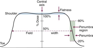
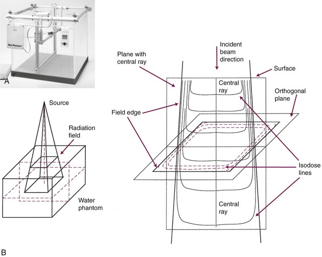
TABLE 6-10 Beam Characteristics from a Dose Profile
| Characteristic | Definition |
|---|---|
| Field size | Distance from field edge to opposite edge at the 50% dose level, with normalization to 100% on the central axis (basically, full-width at half-maximum [FWHM]) |
| Flatness | Deviation in dose level across the width of the field |
| Symmetry | Deviation in dose level for points symmetric about the central axis |
| Penumbra | Dose gradient regions from high to low dose at the beam edge |
The flattening filter and beam steering determine flatness and symmetry in a linear accelerator. Flatness is defined at a reference depth, for instance at a 10-cm depth at the isocenter (SSD = 90 cm). A typical specification is for no more than 3% dose variation across the useful 80% of the field width (see Fig. 6-34). A radiation beam does not have a perfectly sharp edge but instead has a gradient from high to low dose with a rounded “shoulder” and “toe.” This penumbra region is named for geometric shadowing of part of the source, as is the case for 60Co teletherapy beams, which have a large (2 cm) physical source size. However, the penumbra region for linear accelerator beams is mostly a radiation component of secondary electrons and photons scattered from within the field and from the collimators to outside the beam edges. This scatter degrades the beam edge; the dose from the shoulder region scatters outside the beam edge to form the toe. Penumbra is defined as the distance over which the dose falls from 80% to 20% of the central axis dose at the same depth, or at the width of the 90% to 10% dose gradient (see Fig. 6-34).
Various methods exist to measure a radiation beam along lines of equal dose, called isodose lines. In a three-axis water phantom scanner, after determining PDD along the central axis, a certain isodose level is identified in the standard geometry and then tracked to obtain a digital representation of the dosimetric shape of the beam. Figure 6-35 shows sample isodose curves for a plane containing the central ray of a beam and a plane perpendicular to the central ray. The modern water phantom scanning device is computer controlled and has robust software tools for two (2D)- and three-dimensional (3D) renderings and analysis of acquired dose distribution data.
Effect of Energy
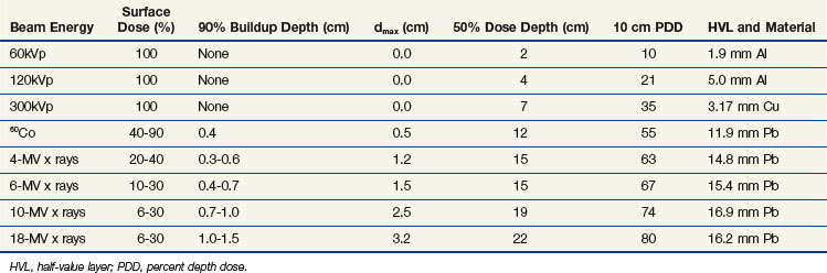
Photon beam characteristics change with beam energy. Representative beam data are presented in Table 6-11, PDDs in Figure 6-36, and isodose curves in Figure 6-37. Several key observations should be considered:
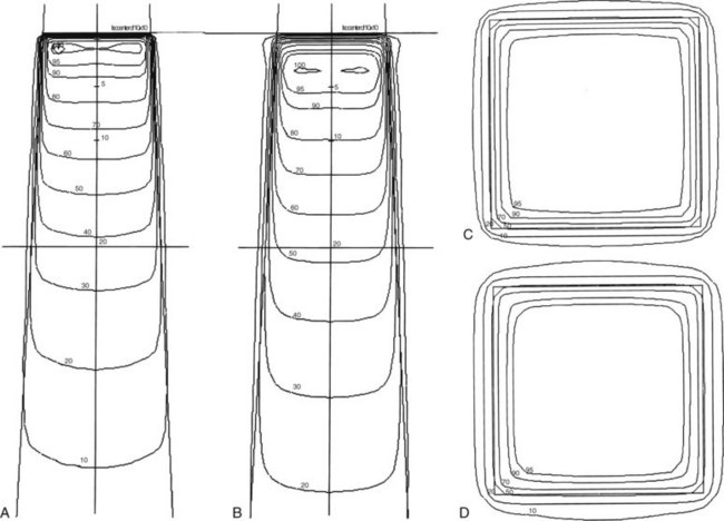
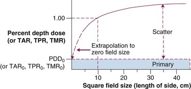
Effect of Field Size
Field size determines the amount of scatter present in the beam, with the following observations:
Penumbra
Beam Modifiers
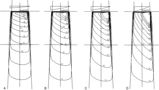
Physical wedges produce skewed isodose lines at fixed angles across the central ray (Fig. 6-39) to compensate for beam angle of incidence, tissue shape, or the trajectory of other treatment beams. Historically, wedge angles of 15, 30, 45, and 60 degrees have been available using physical wedges made of steel or lead. Isodoses show the wedge angle is measured from a perpendicular to the central ray, typically at a depth of 10 cm. A physical wedge produces an attenuated beam that is decreased in absolute dose rate and slightly more penetrating due to beam hardening by the wedge. A commonly available alternative wedging system uses no physical wedge and produces angled isodose lines by scanning one of the independent collimator jaws across the field while the beam is on. This dynamic method does not result in hardening or attenuation of the beam and is called a dynamic, virtual, or soft wedge. Another method to produce an angled beam intensity is to use one physical wedge with the maximum wedge angle of 60 degrees that is left in the beam for various fractions of time to produce wedge angles from 0 (no time in beam) to 60 (full time in beam) degrees.
Compensators attenuate the beam in desired locations to provide dosimetric shaping. A variety of methods exist that include simple and complex approaches.13 Compensators have an important role in dose optimization schemes that include static applications32 as an alternative to dynamic techniques.