[level-membership-for-hematology-oncology-and-palliative-medicine-category]
Quality Assurance in Hematology and Hemostasis Testing
After completion of this chapter, the reader will be able to:
1. Validate and document a new or modified laboratory assay.
2. Define accuracy and calculate accuracy using linear regression to compare to a reference.
3. Compute precision using standard deviation and coefficient of variation.
4. Determine assay linearity using graphical representations and transformations.
5. Discuss analytical limits and analytical specificity.
6. Recount Food and Drug Administration clearance levels for laboratory assays.
7. Compute a reference interval and a therapeutic range for a new or modified assay.
8. Perform internal quality control using controls and moving averages.
9. Participate in periodic external quality assessment.
10. Measure and publish assay clinical efficacy.
11. Compute receiver operating characteristic curves.
12. Periodically assess laboratory staff competence.
13. Provide continuing education programs for laboratory staff.
14. Prepare a quality assurance plan to control for preanalytical and postanalytical variables.
15. List the agencies that regulate hematology and hemostasis quality.
Case Study
1. What do you call the type of error detected in this case?
2. Can you continue to analyze patient samples as long as you subtract 2 g/dL from the results?
3. What aspect of the assay should you first investigate in troubleshooting this problem?
In clinical laboratory science, quality implies the ability to provide accurate, reproducible assay results that offer clinically useful information.1 Because physicians base 70% of their clinical decision making on laboratory results, the results must be reliable. Reliability requires vigilance and effort on the part of all laboratory staff members, and this effort is often directed by an experienced medical laboratory scientist who is a quality assurance and quality control specialist.
Of the terms quality control and quality assurance, quality assurance is the broader concept, encompassing preanalytical, analytical, and postanalytical variables (Box 5-1).2 Quality control processes document assay validity, accuracy, and precision, and should include external quality assessment, reference interval preparation and publication, and lot-to-lot validation.3
Preanalytical variables are addressed in Chapter 3, which discusses blood specimen collection, and in Chapter 45, which includes a section on coagulation specimen management. Postanalytical variables are discussed at the end of this chapter.
The control of analytical variables begins with laboratory assay validation.
Validation of a New or Modified Assay
All new laboratory assays and all assay modifications require validation.4 Validation is comprised of procedures to determine accuracy, specificity, precision, limits, and linearity.5 The results of these procedures are faithfully recorded and made available to on-site assessors upon request.6
Accuracy
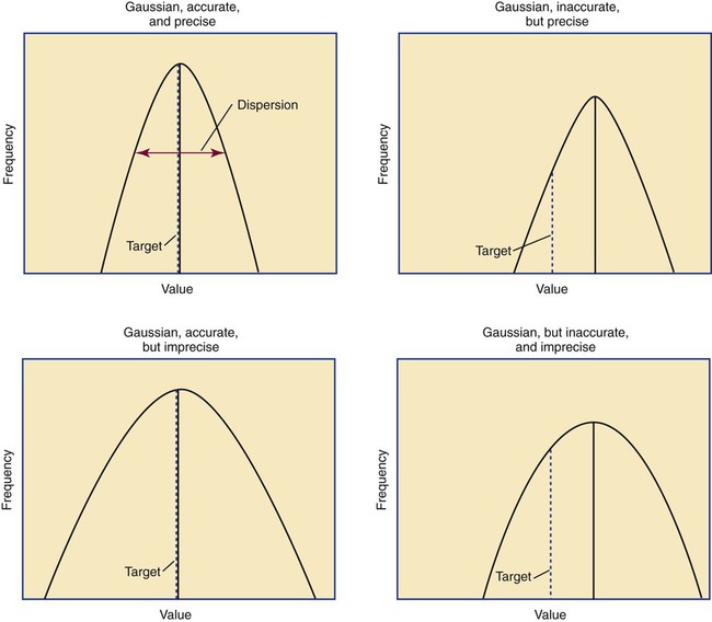
Accuracy is the measure of concurrence or difference between an assay value and the theoretical “true value” of an analyte (Figure 5-1). Some statisticians prefer to define accuracy as the extent of error between the assay result and the true value. Accuracy is easy to define but difficult to establish and maintain.
Unfortunately, in hematology and hemostasis, in which the analytes are often cell suspensions or enzymes, there are just a handful of primary standards: cyanmethemoglobin, fibrinogen, factor VIII, protein C, antithrombin, and von Willebrand factor.7 For scores of analytes, the hematology and hemostasis laboratory scientist relies on calibrators. Calibrators for hematology may be preserved human blood cell suspensions, sometimes supplemented with microlatex particles or nucleated avian red blood cells (RBCs) as surrogates for hard-to-preserve human white blood cells (WBCs). In hemostasis, calibrators may be frozen or lyophilized plasma from healthy human donors. For most analytes it is impossible to prepare “weighed-in” standards; instead, calibrators are assayed using reference methods (“gold standards”) at selected independent expert laboratories. For instance, a vendor may prepare a 1000-L lot of preserved human blood cell suspension, assay for the desired analytes in house, and send aliquots to five laboratories that employ well-controlled reference instrumentation and methods. The vendor obtains blood count results from all five, averages the results, compares them to the in-house values, and publishes the averages as the reference calibrator values. The vendor then distributes sealed aliquots to customer laboratories with the calibrator values published in the accompanying package inserts. Vendors often market calibrators in sets of three or five, spanning the range of assay linearity or the range of potential clinical results.
Determination of Accuracy by Regression Analysis
< ?xml:namespace prefix = "mml" />


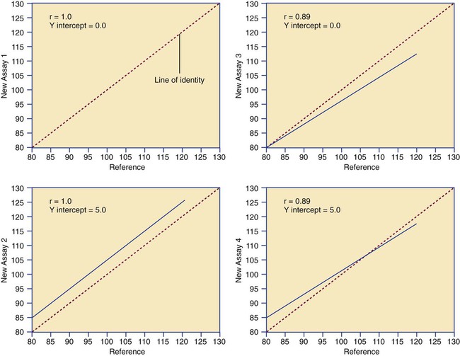
where x and y are the variables; a = intercept between the regression line and the y-axis; b = slope of the regression line; n = number of values or elements; X = first score; Y = second score; ΣXY = sum of the product of first and second scores; ΣX = sum of first scores; ΣY = sum of second scores; ΣX2 = sum of squared first scores. Perfect correlation generates a slope of 1 and a y intercept of 0. Local policy establishes limits for slope and y intercept; for example, many laboratory directors reject a slope of less than 0.9 or an intercept of more than 10% above or below zero (Figure 5-2).
Precision
Unlike determination of accuracy, assessment of precision (dispersion, reproducibility, variation, random error) is a simple validation effort, because it merely requires performing a series of assays on a single sample or lot of reference material.8 Precision studies always assess both within-day and day-to-day variation about the mean and are usually performed on three to five calibration samples, although they may also be performed using a series of patient samples. To calculate within-day precision, the scientist assays a sample at least 20 consecutive times using one reagent batch and one instrument run. For day-to-day precision, at least 10 runs on 10 consecutive days are required. The day-to-day precision study employs the same sample source and instrument but separate aliquots. Day-to-day precision accounts for the effects of different operators, reagents, and environmental conditions such as temperature and barometric pressure.
where (Σx) = the sum of the data values and n = the number of data points collected
The CV% documents the degree of random error generated by an assay, a function of assay stability.
Precision for visual light microscopy leukocyte differential counts on stained blood films is immeasurably broad, particularly for low-frequency eosinophils and basophils.9 Most visual differential counts are performed by reviewing 100 to 200 leukocytes. Although impractical, it would take differential counts of 800 or more leukocytes to improve precision to measurable levels. Automated differential counts generated by profiling instruments, however, provide CV% levels of 5% or lower because these instruments count thousands of cells.
Linearity
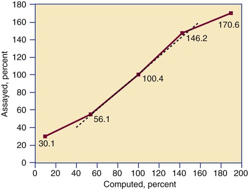
Linearity is the ability to generate results proportional to the calculated concentration or activity of the analyte. The laboratory scientist dilutes a high-end calibrator or patient sample to produce at least five dilutions spanning the full range of assay. The dilutions are then assayed. Computed and assayed results for each dilution are paired and plotted on a linear graph, x scale and y scale, respectively. The line is inspected visually for nonlinearity at the highest and lowest dilutions (Figure 5-3). The acceptable range of linearity is established inboard based on the values at which linearity loss is evident. Although formulas exist for computing the limits of linearity, visual inspection is the accepted practice. Nonlinear graphs may be transformed using semilog or log-log graphs when necessary.
Levels of Laboratory Assay Approval
The U.S. Food and Drug Administration (FDA) categorizes assays as cleared, analyte-specific reagent (ASR) assays, research use only (RUO) assays, and home-brew assays. FDA-cleared assays are approved for the detection of specific analytes and should not be used for off-label applications. Details are given in Table 5-1.
TABLE 5-1
Categories of Laboratory Assay Approval
| Assay Category | Comment |
| Food and Drug Administration cleared | The local institution may use package insert data for linearity and specificity but must establish accuracy and precision. |
| Analyte-specific reagent | Manufacturer may provide individual reagents but not in kit form, and may not provide package insert validation data. Local institution must perform all validation steps. |
| Research use only | Local institution must perform all validation steps. Research use only assays are intended for clinical trials, and carriers are not required to pay. |
| Home brew | Assays devised locally, all validation studies are performed locally. |
Documentation and Reliability
Validation is recorded on standard forms. The Clinical Laboratory Standards Institute (CLSI) and David G. Rhoads Associates (http://www.dgrhoads.com/files1/EE5SampleReports.pdf) provide automated electronic forms. Validation records are stored in prominent laboratory locations and made available to laboratory assessors upon request.
Lot-to-Lot Comparisons
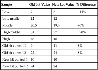
Laboratory managers reach agreements with vendors to sequester kit and reagent lots, which ensures infrequent lot changes, optimistically no more than once a year. The new reagent lot must arrive approximately a month before the laboratory runs out of the old lot so that lot-to-lot comparisons may be completed and differences resolved, if necessary. The scientist uses control or patient samples and prepares a range of analyte dilutions, typically five, spanning the limits of linearity. If the reagent kits provide controls, these are also included, and all are assayed using the old and new reagent lots. Results are charted as illustrated in Table 5-2.
TABLE 5-2
Example of a Lot-to-Lot Comparison
| Sample | Old Lot Value | New Lot Value | % Difference |
| Low | 7 | 6 | −14% |
| Low middle | 12 | 12 | |
| Middle | 20.5 | 19.4 | −5% |
| High middle | 31 | 27 | −20% |
| High | 48 | 48 | |
| Old kit control 1 | 9 | 11 | 8% |
| Old kit control 2 | 22 | 24 | 8% |
| New kit control 1 | 10 | 10 | |
| New kit control 2 | 24 | 24 |
Development of the Reference Interval and Therapeutic Range
Once an assay is validated, the laboratory scientist develops the reference interval (reference range, normal range).10 Most practitioners tend to use the vernacular term normal range; however, reference interval is the preferred term. According to the mathematical definitions, “range” encompasses all assay results from largest to smallest, whereas “interval” is a statistic that trims outliers.
The minimum number of subject samples required to develop a reference interval may be determined using statistical power computations; however, practical limitations prevail.11 For a completely new assay with no currently established reference interval, a minimum of 120 samples is necessary. In most cases, however, the assay manufacturer provides a reference interval on the package insert, and the local laboratory scientist need only assay 30 samples, 15 male and 15 female, to validate the manufacturer’s reference interval, a process called transference. Likewise, the scientist may refer to published reference intervals and, once they are locally validated, transfer them to the institution’s report form.
It is assumed that the population sample subjects employed to generate reference intervals will produce frequency distributions (in laboratory vernacular, histograms) that are normal bell-shaped (gaussian) curves (Figure 5-4). In a gaussian frequency distribution the mean is at the center and the dispersion about the mean is identical in both directions. In many instances, however, biologic frequency distributions are “log-normal” with a “tail” on the high end. For example, it has been assumed for years that the visual reticulocyte percentage reference interval in adults is 0.5% to 1.5%; however, repeated analysis of normal populations in several locations has established it at 0.5% to 2%, owing to a subset of normal subjects whose reticulocyte counts fall at the high end of the range. Scientists may choose to live with a log-normal distribution or they may transform it by replotting the curve using a semilog or log-log graphic display. The decision to transform may arise locally but eventually becomes adopted as a national practice standard.
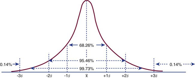
In a normal distribution, the mean ( ) is computed by dividing the sum of the observed values by the number of data points, n, as shown in the equation on page 45. The standard deviation is calculated using the second formula in that equation. A typical reference interval is computed as ±2 standard deviations and assumes that the distribution is normal. The limits at ±2 standard deviations encompass 95.46% of normal results, known as the 95% confidence interval. This implies that 4.54% of theoretically normal results fall outside the interval. A standard deviation computed from a nongaussian distribution may turn out to be too narrow to reflect the true reference interval and may thus encompass fewer than 95% of theoretical normal values and generate a number of false positives. Assays with high CV% values have high levels of random error reflected in a broad curve; low CV% assays with “tight” dispersal have smaller random error and generate a narrow curve, as illustrated in Figure 5-1. The breadth of the curve may also reflect biologic variation in values of the analyte.
Internal Quality Control
Controls
Laboratory managers prepare, or more often purchase, assay controls. Although it may appear similar, a control is wholly distinct from a calibrator. Indeed, cautious laboratory directors may insist that controls be purchased from distributors different from those who supply their calibrators. As discussed in the section Validation of a New or Modified Assay, calibrators are used to adjust instrumentation or to develop a standard curve. Calibrators are assayed by a reference method in expert laboratories and their assigned value is certified. Controls are used independently of the calibration process so that systematic errors caused by deterioration of the calibrator or a change in the analytical process can be detected through internal quality control. This process is continuous and is called calibration verification.12 Compared with calibrators, control materials are inexpensive and are comprised of the same matrix as patient samples except for preservatives or freezing that provide a long shelf life. Controls provide known values and are sampled directly alongside patient specimens to accomplish within-run assay validation. In nearly all instances, two controls are required per test run, one in the normal range and the other in an expected abnormal range. For some assays there is reason to select controls whose values are near the interface of normal and abnormal. In institutions that perform continuous runs, the controls should be run at least once per shift, for instance, at 7 am, 3 pm, and 11 pm. In laboratories where assay runs are discrete events, two controls are assayed with each run.
Control results must fall within predetermined dispersal limits, typically ±2 standard deviations. Control manufacturers provide limits; however, local laboratory scientists must validate and transfer manufacturer limits or establish their own, usually by computing standard deviation from the first 20 control assays. Whenever the result for a control is outside the limits the run is rejected and the cause is found and corrected. The steps for correction are listed in Table 5-3.
TABLE 5-3
Steps Used to Correct an Out-of-Control Assay Run
| Step | Description |
| 1. Reassay | When a limit of ±2 standard deviations is used, 5% of expected assay results fall above or below the limit. |
| 2. Prepare new control and reassay | Controls may deteriorate over time when exposed to adverse temperatures or subjected to conditions causing evaporation. |
| 3. Prepare fresh reagents and reassay | Reagents may have evaporated or become contaminated. |
| 4. Recalibrate instrument | Instrument may require repair. |
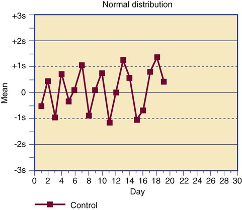
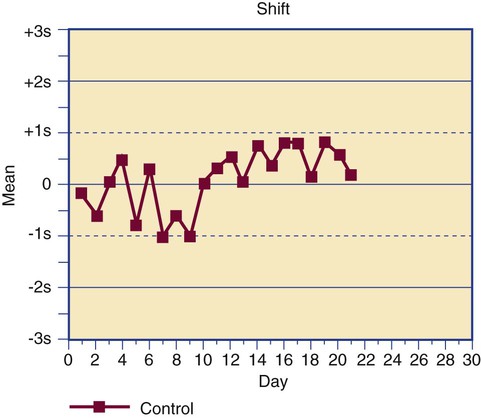
Control results are plotted on a Levey-Jennings chart that displays each data point in comparison to the mean and limits (Figure 5-5).13 The Levey-Jennings chart assumes that the control results distribute in a gaussian manner and provide limits at 1, 2, and 3 standard deviations about the mean. In addition to being analyzed for single-run errors, the data points are examined for sequential errors over time (Figure 5-6). Both single-run and long-term control variation are a function of assay dispersion or random error and reflect the CV% of an assay.
Dr. James Westgard has established a series of internal quality control rules that are routinely applied to long-term deviations, called the Westgard rules.14 The rules were developed for assays that employ primary standards, but a few Westgard rules that are the most useful in hematology and hemostasis laboratories are provided in Table 5-4, along with the appropriate actions to be taken.15
TABLE 5-4
Westgard Rules Employed in Hematology and Hemostasis
| 12s or 22s | A single control assay or two control assays are outside the ±2 standard deviation limit. Assay results are held until the error is identified using the steps in Table 5-3. Variations of this rule are 13s and 41s. |
| 13s | A single control assay is outside the ±3 standard deviation limit. Assay results are held until the error is identified using the steps in Table 5-3. |
| R4s | Two consecutive control values are more than 4 standard deviations apart. Assay results are held until the error is identified using the steps in Table 5-3. |
| Shift | A series of at least 10 control values remain within the dispersal limits but are consistently above or below the mean. Use of the assay is suspended until the cause is found; often it is an instrument calibration issue that has introduced a constant systematic error (bias). |
| Trend | A series of at least 10 control values changes in a consistent direction. Use of the assay is suspended until the cause is found; often it is an instrument calibration issue that has introduced a systematic proportional error. |
Moving Average ( ) of the Red Blood Cell Indices
In 1974, Dr. Brian Bull proposed a method of employing patient RBC indices to monitor the stability of hematology analyzers, recognizing that the RBC indices mean cell volume (MCV), mean cell hemoglobin (MCH), and mean cell hemoglobin concentration (MCHC) remain constant on average despite individual patient variations.16 Each consecutive sequence of 20 patient RBC index assay results is collected and treated by the moving average formula, which accumulates, “smoothes,” and trims data to reduce the effect of outliers. Each trimmed 20-sample mean,  , is plotted on a Levey-Jennings chart and tracked for trends and shifts using Westgard rules. The formula has been automated and embedded in the circuitry of all hematology analyzers, which provide a Levey-Jennings graph for MCV, MCH, and MCHC. The moving average concept has been generalized to WBC and platelet counts and to some clinical chemistry analytes, albeit with moderate success.
Delta Checks
The δ-check system compares a current analyte result with the result from the most recent previous analysis for the same patient.17 Patient values remain relatively consistent over time unless there is an intervention. A result that fails a δ check is investigated for intervention or a profound change in the patient’s condition subsequent to the previous analysis. If there is no ready explanation, the failed δ check may indicate an analytical error or mislabeled specimen. Results that fail a δ check are sequestered until the cause is found. Not all assays are amenable to δ checking; only analytes known to show little intraindividual variation are checked. These include MCV and RBC distribution width. In hemostasis, the prothrombin time and INR are checked. Action limits for δ checks are based on clinical impression and are assigned by hematology and hemostasis laboratory directors in collaboration with the house and laboratory staff. Computerization is essential, and δ checks are designed only to identify gross errors, not changes in random error, or shifts or trends. There is no regulatory requirement for δ checks.
Measurement of Clinical Efficacy
Since 1940 and before, surgeons have used the bleeding time test to predict the risk of intraoperative hemorrhage. The laboratory scientist or phlebotomist activates an automated lancet to make a 5-mm long, 1-mm deep incision in the volar surface of the forearm and, using a filter paper to soak up the blood, times the interval from the initial incision to bleeding cessation, normally 2 to 9 minutes. The test is simple and logical, and for over 50 years experts have claimed that if the incision bleeds for longer than 9 minutes, there is a risk of surgical bleeding. In the 1990s clinical researchers compared normal and prolonged bleeding times with instances of intraoperative bleeding and found to their surprise that prolonged bleeding time predicted only 50% of intraoperative bleeds.18,19 The other 50% occurred despite a normal bleeding time. Thus the positive predictive value of the bleeding time for intraoperative bleeding was 50%, the same as the probability of obtaining heads (or tails) in tossing a coin. Today the bleeding time test is widely agreed to have no clinical relevance and is obsolete.
Like the bleeding time test, many time-honored hematology and hemostasis assays gain credibility on the basis of expert opinion. Now, however, besides being valid, accurate, linear, and precise, a new or modified assay must be clinically effective.20 To compute clinical efficacy, the scientist uses a series of samples from normal healthy subjects, called controls, and patients who conclusively possess a disease or condition. The patient’s diagnosis is based on clinical outcomes, discharge diagnosis notes, or the results of existing laboratory tests, excluding the new assay. The new assay is then applied to samples from both the normal and disease groups to assess its efficacy.
In a perfect world, the laboratory scientist sets the discrimination threshold at the 95% confidence interval limit (±2 standard deviations) of the reference interval. When this threshold is used, the test will hopefully yield a positive result (e.g., elevated or reduced level) in every instance of disease and a negative result (within the reference interval) in all normal control subjects. In reality, there is always overlap: a “gray area” in which some positive test results are generated by normal samples (false positives) and some negative results are generated by samples from patients with disease (false negatives). False positives cause unnecessary anxiety, follow-up expense, and erroneous diagnostic leads—worrisome, expensive, and time consuming, but not fatal. False negatives fail to detect the disease and may delay treatment, which is potentially life-threatening. The laboratory scientist employs clinical efficacy computations to establish laboratory assay efficacy and minimize both false positives and false negatives (Table 5-5). Clinical efficacy testing includes determination of diagnostic sensitivity and specificity, and positive and negative predictive value, as well as receiver operating characteristic analysis.
TABLE 5-5
Clinical Efficacy Definitions and Binary Display
| True positive | Assay correctly identifies a disease or condition in those who have it. |
| False positive | Assay incorrectly identifies disease when none is present. |
| True negative | Assay correctly excludes a disease or condition in those without it. |
| False negative | Assay incorrectly excludes disease when it is present. |
| Normal (Control Sample) | Disease or Condition (Patient Sample) | |
| Assay is negative | True negative | False negative |
| Assay is positive | False positive | True positive |
To start a clinical efficacy study the scientist selects normal control samples and samples from people proven to have the disease or condition addressed by the assay. To make the discussion easy, assume that 50 samples of each are chosen. All are assayed, and the results turn out as shown in Table 5-6.
TABLE 5-6
| Normal (Control Sample) | Disease or Condition (Patient Sample) | |
| Assay is negative | True negative: 45 | False negative: 5 |
| Assay is positive | False positive: 5 | True positive: 45 |
The scientist next computes clinical sensitivity and specificity and positive and negative predictive value as shown in Table 5-7.
TABLE 5-7
Clinical Efficacy Computations
| Statistic | Definition | Formula | Example |
| Sensitivity | Proportion with the disease who have a positive test result | Sensitivity (%) = TP/(TP + FN) × 100 | 45/(45 + 5) × 100 = 90% |
| Distinguish clinical sensitivity from analytical sensitivity. Analytical sensitivity is a measure of the smallest increment of the analyte that can be distinguished by the assay. | |||
| Specificity | Proportion without the disease who have a negative test result | Specificity (%) = TN/(TN + FP) × 100 | 45/(45 + 5) × 100 = 90% |
| Distinguish clinical specificity from analytical specificity. Analytical specificity is the ability of the assay to distinguish the analyte from interfering substances. | |||
| Positive predictive value (PPV) | Proportion with a disease who have a positive test result compared with all subjects who have a positive test result | PPV (%) = TP/(TP + FP) × 100 | 45/(45 + 5) × 100 = 90% |
| The positive predictive value predicts the probability that an individual with a positive assay result has the disease or condition. | |||
| Negative predictive value (NPV) | Proportion without a disease who have a negative test result compared with all subjects who have a negative test result | NPV (%) = TN/(TN + FN) × 100 | 45/(45 + 5) × 100 = 90% |
| The negative predictive value predicts the probability that an individual with a negative assay result does not have the disease or condition. | |||
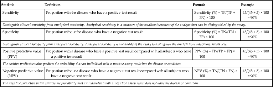
FN, False negative; FP, false positive; TN, true negative; TP, true positive.
Receiver Operating Characteristic Curve
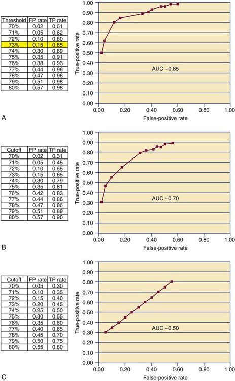
A receiver operating characteristic (ROC) curve or ROC analysis is a further refinement of clinical efficacy testing that may be employed when the assay being validated generates a continuous variable.21 In clinical efficacy testing as described earlier, the ±2 standard deviation limit of the reference interval is used as the threshold for discriminating a positive from a negative test result. Often the “true” threshold varies from the ±2 standard deviation limit. Using ROC analysis, the discrimination threshold is adjusted by increments of 1, and the true-positive and false-positive rates are recomputed for each new threshold level. The threshold that is selected is the one that provides the largest true-positive and smallest false-positive rate (Figure 5-7). A line graph is generated plotting true positives on the y-axis and false positives on the x-axis. The overall efficacy of the assay is assessed by measuring the area under the curve. If the area under the curve is 0.5, the curve is at the line of identity between false and true positives and provides no discrimination. Most agree that a clinically useful assay should have an area under the curve of 0.85 or higher.
Laboratory Staff Competence
Staff integrity and professional staff competence are the keys to assay reliability. In the United States, 12 states have medical laboratory personnel licensure laws. In these states, only licensed laboratory professionals may be employed in medical center or reference laboratories. In nonlicensure states conscientious laboratory directors employ only nationally certified professionals. Certification is available from the American Society for Clinical Pathology Board of Certification in Chicago, Illinois. Studies of outcomes and laboratory errors demonstrate that laboratories that employ only licensed or certified professionals produce the most reliable assay results.22,23
Continuing Education
The American Society for Clinical Pathology Board of Certification and state medical licensure boards require professional personnel to participate in and document continuing education for periodic recertification or relicensure. Continuing education is delivered in the form of journal articles, case studies, distance learning seminars, and professional meetings. Medical centers offer periodic internal continuing education opportunities (in-service education) in the form of grand rounds, lectures, seminars, and participative educational events. Presentation and discussion of local cases is particularly effective. Continuing education maintains the critical skills of laboratory scientists and provides opportunities to learn about new clinical and technical approaches. The Colorado Association for Continuing Medical Laboratory Education (http://www.cacmle.org), the American Society for Clinical Laboratory Science (http://www.ascls.org), the American Society for Clinical Pathology (http://www.ascp.org), the American Society of Hematology (http://www.hematology.org), the National Hemophilia Foundation (http://www.hemophilia.org), CLOT-ED (http://www.clot-ed.com), and the Fritsma Factor (http://www.fritsmafactor.com) are examples of scores of organizations that direct their activities toward quality continuing education in hematology and hemostasis.
Quality Assurance Plan: Preanalytical and Postanalytical
In addition to keeping analytical quality control records, U.S. agencies require laboratory directors to maintain records of preanalytical and postanalytical quality assurance and quality improvement efforts.24 Although not exhaustive, Table 5-8 lists and characterizes a number of examples of preanalytical quality efforts, and Table 5-9 provides a review of postanalytical components. All quality assurance plans include objectives, sources of authority, scope of services, an activity calendar, corrective action, periodic evaluation, standard protocol, personnel involvement, and methods of communication.25
TABLE 5-8
Preanalytical Quality Assurance Components and the Laboratory’s Responsibility
| Preanalytical Component | Laboratory Staff Responsibility |
| Test orders | Conduct continuous utilization reviews to ensure that physician laboratory orders are comprehensive and appropriate to patient condition. Inform physician about laboratory test availability and ways to avoid unnecessary orders. Reduce unnecessary repeat testing. |
| Test request forms |
Is the patient correctly identified, prepared, and available for specimen collection? Is fasting and therapy status appropriate for laboratory testing?
Is the tourniquet correctly applied and released at the right time? Are venipuncture sites appropriately cleansed? Are timed specimens collected at the specified intervals? Are specimen tubes collected in the specified order? Are additive tubes properly mixed? Are specimen tubes labeled correctly?
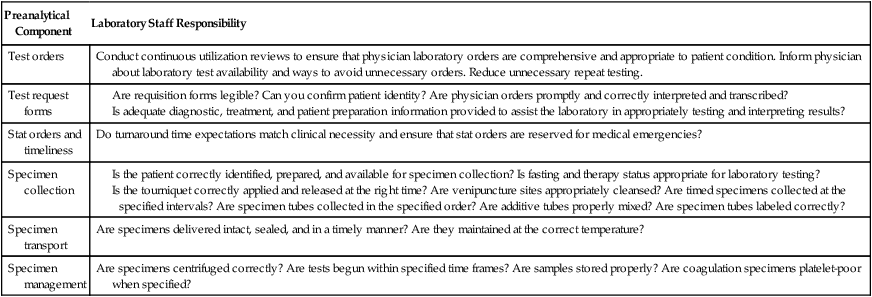
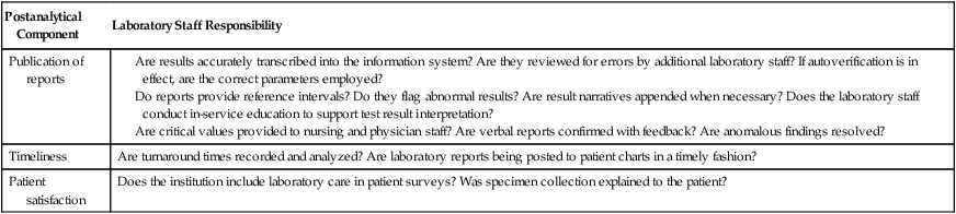
TABLE 5-9
Postanalytical Quality Assurance Components and the Laboratory’s Responsibility
| Postanalytical Component | Laboratory Staff Responsibility |
| Publication of reports |
Are results accurately transcribed into the information system? Are they reviewed for errors by additional laboratory staff? If autoverification is in effect, are the correct parameters employed? Do reports provide reference intervals? Do they flag abnormal results? Are result narratives appended when necessary? Does the laboratory staff conduct in-service education to support test result interpretation? Are critical values provided to nursing and physician staff? Are verbal reports confirmed with feedback? Are anomalous findings resolved? |
| Timeliness | Are turnaround times recorded and analyzed? Are laboratory reports being posted to patient charts in a timely fashion? |
| Patient satisfaction | Does the institution include laboratory care in patient surveys? Was specimen collection explained to the patient? |
Agencies that Address Hematology and Hemostasis Quality
• Clinical and Laboratory Standards Institute (CLSI) (http://www.clsi.org), 940 West Valley Road, Suite 1400, Wayne, PA 19087. Produces guidelines and standards for laboratory practice. Hemostasis documents include H21-A5, H30-A2, and H47–H58. Hematology standards include H02-A4, H07-A3, and H22–H46. Clinical efficacy method evaluation, mostly EP suffix standards; quality assurance and quality management systems, mostly GP suffix standards are available.
• Center for Medicare and Medicaid Services (CMS) (http://www.cms.hhs.gov), 7500 Security Boulevard, Baltimore, MD 21244. Administers the laws and rules developed from the Clinical Laboratory Improvement Amendments of 1988. Establishes Current Procedural Terminology (CPT) codes, reimbursement rules, and test complexity.
• College of American Pathologists (CAP) (http://www.cap.org/apps/cap.portal), 325 Waukegan Road, Northfield, IL 60093. Laboratory accreditation, proficiency testing, and quality assurance programs; laboratory education, reference resources, and e-lab solutions.
• Joint Commission (http://www.jointcommission.org), One Renaissance Boulevard, Oakbrook Terrace, IL 60181. Accreditation and certification programs.
Summary
• Each new assay or assay modification must be validated for accuracy, precision, linearity, specificity, and lower limit of detection ability. In the hematology and hemostasis laboratory, accuracy validation usually requires a series of calibrators, although it may be accomplished by using a number of patient specimens and comparing results with those obtained using a reference method. In all cases, accuracy is established using the Student t-test and linear regression.
• Precision is established by using repeated within-day and day-to-day assays, then computing the mean, standard deviation, and coefficient of variation of the results.
• Assay linearity, specificity, and lower limit of detection are usually provided by the vendor; however, many laboratory managers require that these parameters be revalidated locally.
• Internal quality control is accomplished by assaying controls with each test run. Control results are compared with action limits, usually the mean of the control assay ±2 standard deviations. If the control value is outside the limits, use of the assay is suspended and the scientist begins troubleshooting. Control results are plotted on Levey-Jennings charts and examined for drift and trends. Internal quality control is enhanced through the use of the moving average algorithm.
• All conscientious laboratory directors subscribe to an external quality assessment system, also known as proficiency testing or proficiency surveys. External quality assessment enables the director to compare selected assay results with other laboratory results, nationally and internationally, as a further check of accuracy. Maintaining a good external quality assessment record is essential to laboratory accreditation. Most U.S. states require external quality assessment for laboratory licensure.
• All laboratory assays are analyzed for clinical efficacy, sensitivity, and specificity, including their true-positive and true-negative rates, and positive and negative predictive values. Highly sensitive assays may be used for population screening, but may lack good discrimination. Specific assays may be used to confirm a condition, but generate a number of false negatives. Clinical efficacy computations expand to include receiver operating characteristic curve analysis.
• Thoughtful laboratory managers hire only certified or licensed medical laboratory scientists and technicians and provide regular individual proficiency tests that are correlated with in-service education. Staff are encouraged to participate in continuing education activities and in-house discussion of cases. Quality laboratories provide resources for staff to pursue higher education.
• The laboratory director maintains a protocol for assessing and improving upon preanalytical and postanalytical variables and finds means to communicate enhancements to other members of the health care team.
Review Questions
1. You validate a new assay using linear regression to compare assay calibrator results with the distributor’s published calibrator results. The slope is 0.95 and y intercept is +10%. What type of error is present?
2. The acceptable hemoglobin control value range is 13 ± 0.4 g/dL. The control is assayed five times and produces the following five results:
| 12.0 g/dL | 12.3 g/dL | 12.0 g/dL | 12.2 g/dL | 12.1 g/dL |

3. A WBC count control has a mean value of 6000/mcL and a standard deviation of 300/mcL. What is the 95.5% confidence interval?
4. The ability of an assay to distinguish the targeted analyte from interfering substances within the sample matrix is called:
5. The laboratory purchases reagents from a manufacturer and develops an assay using standard references. What FDA category is this assay?
6. A laboratory scientist measures prothrombin time for plasma aliquots from 15 normal males and 15 normal females. She computes the mean and 95.5% confidence interval and notes that they duplicate the manufacturer’s statistics within 5%. This procedure is known as:
7. You purchase a preserved whole blood specimen from a distributor who provides the mean values for several complete blood count analytes. What is this specimen called?
8. You perform a clinical efficacy test and get the following results:
| Normal (Control Sample) | Disease or Condition (Patient Sample) | |
| Assay is negative | 40 | 5 |
| Assay is positive | 10 | 45 |
What is the number of false-negative results?
9. What agency provides external quality assurance (proficiency) surveys and laboratory accreditation?
a. College of American Pathologists (CAP)
b. Clinical Laboratory Improvement Advisory Committee (CLIAC)
10. What agency provides continuing medical laboratory education?
a. Clinical Laboratory Improvement Advisory Committee (CLIAC)
b. Center for Medicare and Medicaid Services (CMS)
c. Colorado Association for Continuing Medical Laboratory Education (CACMLE)
11. Regular review of blood specimen collection quality is an example of:
[/level-membership-for-hematology-oncology-and-palliative-medicine-category][not-level-membership-for-hematology-oncology-and-palliative-medicine-category]
Quality Assurance in Hematology and Hemostasis Testing
After completion of this chapter, the reader will be able to:
1. Validate and document a new or modified laboratory assay.
2. Define accuracy and calculate accuracy using linear regression to compare to a reference.
3. Compute precision using standard deviation and coefficient of variation.
4. Determine assay linearity using graphical representations and transformations.
5. Discuss analytical limits and analytical specificity.
6. Recount Food and Drug Administration clearance levels for laboratory assays.
7. Compute a reference interval and a therapeutic range for a new or modified assay.
8. Perform internal quality control using controls and moving averages.
9. Participate in periodic external quality assessment.
10. Measure and publish assay clinical efficacy.
11. Compute receiver operating characteristic curves.
12. Periodically assess laboratory staff competence.
13. Provide continuing education programs for laboratory staff.
14. Prepare a quality assurance plan to control for preanalytical and postanalytical variables.
15. List the agencies that regulate hematology and hemostasis quality.
Case Study
1. What do you call the type of error detected in this case?
2. Can you continue to analyze patient samples as long as you subtract 2 g/dL from the results?
3. What aspect of the assay should you first investigate in troubleshooting this problem?
In clinical laboratory science, quality implies the ability to provide accurate, reproducible assay results that offer clinically useful information.1 Because physicians base 70% of their clinical decision making on laboratory results, the results must be reliable. Reliability requires vigilance and effort on the part of all laboratory staff members, and this effort is often directed by an experienced medical laboratory scientist who is a quality assurance and quality control specialist.
Of the terms quality control and quality assurance, quality assurance is the broader concept, encompassing preanalytical, analytical, and postanalytical variables (Box 5-1).2 Quality control processes document assay validity, accuracy, and precision, and should include external quality assessment, reference interval preparation and publication, and lot-to-lot validation.3
Preanalytical variables are addressed in Chapter 3, which discusses blood specimen collection, and in Chapter 45, which includes a section on coagulation specimen management. Postanalytical variables are discussed at the end of this chapter.
The control of analytical variables begins with laboratory assay validation.
Validation of a New or Modified Assay
All new laboratory assays and all assay modifications require validation.4 Validation is comprised of procedures to determine accuracy, specificity, precision, limits, and linearity.5 The results of these procedures are faithfully recorded and made available to on-site assessors upon request.6
Accuracy
Accuracy is the measure of concurrence or difference between an assay value and the theoretical “true value” of an analyte (Figure 5-1). Some statisticians prefer to define accuracy as the extent of error between the assay result and the true value. Accuracy is easy to define but difficult to establish and maintain.
Unfortunately, in hematology and hemostasis, in which the analytes are often cell suspensions or enzymes, there are just a handful of primary standards: cyanmethemoglobin, fibrinogen, factor VIII, protein C, antithrombin, and von Willebrand factor.7 For scores of analytes, the hematology and hemostasis laboratory scientist relies on calibrators. Calibrators for hematology may be preserved human blood cell suspensions, sometimes supplemented with microlatex particles or nucleated avian red blood cells (RBCs) as surrogates for hard-to-preserve human white blood cells (WBCs). In hemostasis, calibrators may be frozen or lyophilized plasma from healthy human donors. For most analytes it is impossible to prepare “weighed-in” standards; instead, calibrators are assayed using reference methods (“gold standards”) at selected independent expert laboratories. For instance, a vendor may prepare a 1000-L lot of preserved human blood cell suspension, assay for the desired analytes in house, and send aliquots to five laboratories that employ well-controlled reference instrumentation and methods. The vendor obtains blood count results from all five, averages the results, compares them to the in-house values, and publishes the averages as the reference calibrator values. The vendor then distributes sealed aliquots to customer laboratories with the calibrator values published in the accompanying package inserts. Vendors often market calibrators in sets of three or five, spanning the range of assay linearity or the range of potential clinical results.
Determination of Accuracy by Regression Analysis
< ?xml:namespace prefix = "mml" />
where x and y are the variables; a = intercept between the regression line and the y-axis; b = slope of the regression line; n = number of values or elements; X = first score; Y = second score; ΣXY = sum of the product of first and second scores; ΣX = sum of first scores; ΣY = sum of second scores; ΣX2 = sum of squared first scores. Perfect correlation generates a slope of 1 and a y intercept of 0. Local policy establishes limits for slope and y intercept; for example, many laboratory directors reject a slope of less than 0.9 or an intercept of more than 10% above or below zero (Figure 5-2).
Precision
Unlike determination of accuracy, assessment of precision (dispersion, reproducibility, variation, random error) is a simple validation effort, because it merely requires performing a series of assays on a single sample or lot of reference material.8 Precision studies always assess both within-day and day-to-day variation about the mean and are usually performed on three to five calibration samples, although they may also be performed using a series of patient samples. To calculate within-day precision, the scientist assays a sample at least 20 consecutive times using one reagent batch and one instrument run. For day-to-day precision, at least 10 runs on 10 consecutive days are required. The day-to-day precision study employs the same sample source and instrument but separate aliquots. Day-to-day precision accounts for the effects of different operators, reagents, and environmental conditions such as temperature and barometric pressure.
where (Σx) = the sum of the data values and n = the number of data points collected
The CV% documents the degree of random error generated by an assay, a function of assay stability.
Precision for visual light microscopy leukocyte differential counts on stained blood films is immeasurably broad, particularly for low-frequency eosinophils and basophils.9 Most visual differential counts are performed by reviewing 100 to 200 leukocytes. Although impractical, it would take differential counts of 800 or more leukocytes to improve precision to measurable levels. Automated differential counts generated by profiling instruments, however, provide CV% levels of 5% or lower because these instruments count thousands of cells.
Linearity
Linearity is the ability to generate results proportional to the calculated concentration or activity of the analyte. The laboratory scientist dilutes a high-end calibrator or patient sample to produce at least five dilutions spanning the full range of assay. The dilutions are then assayed. Computed and assayed results for each dilution are paired and plotted on a linear graph, x scale and y scale, respectively. The line is inspected visually for nonlinearity at the highest and lowest dilutions (Figure 5-3). The acceptable range of linearity is established inboard based on the values at which linearity loss is evident. Although formulas exist for computing the limits of linearity, visual inspection is the accepted practice. Nonlinear graphs may be transformed using semilog or log-log graphs when necessary.
Levels of Laboratory Assay Approval
The U.S. Food and Drug Administration (FDA) categorizes assays as cleared, analyte-specific reagent (ASR) assays, research use only (RUO) assays, and home-brew assays. FDA-cleared assays are approved for the detection of specific analytes and should not be used for off-label applications. Details are given in Table 5-1.
TABLE 5-1
Categories of Laboratory Assay Approval
| Assay Category | Comment |
| Food and Drug Administration cleared | The local institution may use package insert data for linearity and specificity but must establish accuracy and precision. |
| Analyte-specific reagent | Manufacturer may provide individual reagents but not in kit form, and may not provide package insert validation data. Local institution must perform all validation steps. |
| Research use only | Local institution must perform all validation steps. Research use only assays are intended for clinical trials, and carriers are not required to pay. |
| Home brew | Assays devised locally, all validation studies are performed locally. |
Documentation and Reliability
Validation is recorded on standard forms. The Clinical Laboratory Standards Institute (CLSI) and David G. Rhoads Associates (http://www.dgrhoads.com/files1/EE5SampleReports.pdf) provide automated electronic forms. Validation records are stored in prominent laboratory locations and made available to laboratory assessors upon request.
Lot-to-Lot Comparisons
Laboratory managers reach agreements with vendors to sequester kit and reagent lots, which ensures infrequent lot changes, optimistically no more than once a year. The new reagent lot must arrive approximately a month before the laboratory runs out of the old lot so that lot-to-lot comparisons may be completed and differences resolved, if necessary. The scientist uses control or patient samples and prepares a range of analyte dilutions, typically five, spanning the limits of linearity. If the reagent kits provide controls, these are also included, and all are assayed using the old and new reagent lots. Results are charted as illustrated in Table 5-2.
TABLE 5-2
Example of a Lot-to-Lot Comparison
| Sample | Old Lot Value | New Lot Value | % Difference |
| Low | 7 | 6 | −14% |
| Low middle | 12 | 12 | |
| Middle | 20.5 |
