Chapter 31 Physics and technology of ultrasound
What is ultrasound?
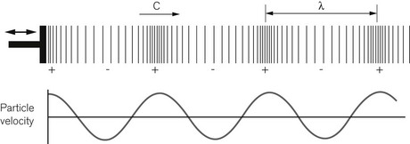
Diagnostic ultrasound uses high-frequency sound waves sent into the body, to build up an image of the anatomical structures within from the detected echoes. A sound wave is what is known as a longitudinal compression wave (Fig. 31.1). It may be formed by some sort of piston, a loudspeaker for example, that pushes forward onto the molecules of air in front of it forming a region of higher density and pressure immediately in front of the piston. These molecules then push on to the molecules in front of them and so on, so the pulse of high pressure starts to move forward away from the piston. Meanwhile the piston moves backwards creating a region of low density and pressure in the molecules in front of it. By repeatedly moving forwards and backwards, a succession of high pressure followed by low-pressure regions move away from the piston forming a longitudinal pressure wave, a sound wave. If we were able to see just one molecule in front of the piston, we would see it oscillate forwards and backwards about an average position, like a child on a swing. Hence the molecules of the medium carrying the sound wave stay in approximately the same place, but the disturbance, i.e. the change in pressure, travels out, away from the piston.

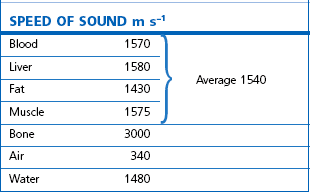
For any given medium the speed of sound is constant. This means that a high frequency implies a short wavelength and low frequency a long wavelength. Table 31.1 gives examples of the speed of sound travelling through different tissues, and also air and water. The speed of sound depends on how rigid a material is, that is: how strongly the molecules are bound together, and how massive the molecules are, i.e. how easy they are to move. In air the molecules are very poorly connected with one another and the speed of sound is low at 340 m s−1. Bone is a very rigid material and the speed of sound is fast at 3000 m s−1. Water has a speed of sound somewhere in between these figures: 1480 m s−1 at 20°C. The speed of sound for all the soft tissues in the body shows little variation, with values being not very different from that of water. For the purposes of image formation using ultrasound, the speed of sound in the different soft tissues can be approximated by an average value of 1540 m s−1 (+/− 10%) and this is the value of c that is used for ultrasound imaging.
Ultrasound is any sound with a frequency that is higher than the range of our hearing, which in a young person runs from 20 Hz to 20 kHz. For diagnostic imaging the frequencies used are far higher than anything we can hear and are in the range of 3–15 MHz. Putting these frequencies into the speed of sound equation, and using a speed of sound of 1540 m s−1, we see that the wavelength of ultrasound in soft-tissue ranges from 0.5 to 0.1 mm. The reason for using these very high frequencies is to produce narrow beams of sound (see below) and to image with high resolution so that small structures within the body can be viewed.
Pulse echo principle
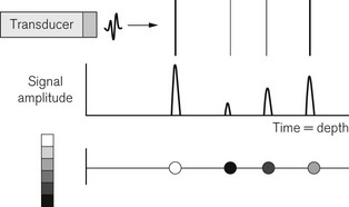
Ultrasound imaging uses the pulse-echo principle in a similar manner to sonar on a submarine (Fig. 31.2). A short pulse of sound is sent into the body and echoes reflected off anatomical structures in the tissues return to the transducer. The received signals are used to build up an image of the anatomy. The pulse transmitted into the body is typically only two to three cycles long and lasts just less than 1 µs. If the transducer were to produce a continuous wave of sound there would be a beam of sound travelling into the body as described before (Fig. 31.2A). When a short pulse is used, the pulse travels down the same beam shape. In other words, the ultrasound beam can be thought of as the corridor down which the pulse travels and from which the echoes will arise. Any tissue lying outside the beam, in general will not see the pulse and not send any echoes back to the transducer. The pulse travels at 1540 m s−1 towards the target at some depth (d) in tissue. An echo is reflected from the target which travels back to the transducer at the same speed. The echo pulse has, therefore, travelled the distance twice, from the transducer to the target and back, and the time of arrival of the echo back at the transducer Δt is given by equation:
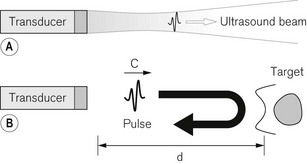

For a speed of sound of 1540 ms−1, the go and return time of the pulse is 13 µs per cm. Because the machine can assume a constant value of sound of 1540 m s−1, the scanner can use the timing of echo arrival to position echoes in the image and mark the depth axis of the display in centimetres depth.
The ultrasound transducer
The transducer plays the role of the piston in producing the sound wave (Fig. 31.3A). It converts electrical energy into sound energy and vice versa. Ultrasound transducers use a piezoelectric material to produce a sound wave. This is a material having the property that when an electrical voltage is placed across it, it changes shape and contracts in the direction of the applied voltage. If the polarity of the voltage is reversed, the piezoelectric material expands. The process is reciprocal. If the material is squeezed, a voltage forms across it, and if the material is stretched, the voltage produced has the opposite polarity. A naturally occurring example of a piezoelectric material is quartz. This is what forms the resonator in a quartz clock. Ultrasound transducers usually use a ceramic material called lead zirconate titanate (PZT). A piece of this material is used whose thickness is such that it has a natural resonance at the frequency of ultrasound we wish to use, say 10 MHz. The PZT element has electrodes on its faces. When a high-voltage spike is applied to the electrodes the PZT is made to rapidly contract. It then vibrates at its resonant frequency, like an empty wine glass struck with a fingernail. In order to make a very short pulse the back of the PZT element has a layer of sound absorbing material (backing layer) stuck to it to reduce the ringing (Fig. 31.3B). This shortens the pulse in a similar way to striking the wine glass, but with the fingers of the other hand pinching the rim of the glass.
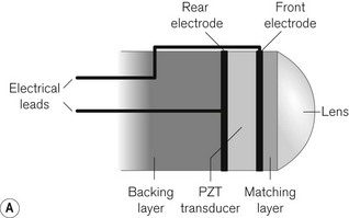
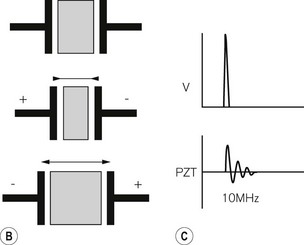
Image formation
The way a modern ultrasound scanner forms an image may be considered in three stages. Firstly, if an ultrasound beam is directed into the body towards a series of reflecting targets the output from the received echoes can be displayed as a series of peaks whose time of arrival depends on the depth equation and whose amplitude depends on the reflecting strength of the targets. A strong reflector gives a high amplitude signal and a weak reflector gives a small signal. This type of display is known as an A-mode or amplitude mode display (Fig. 31.4).
The final step is to sweep the beam through the tissue and to repeatedly interrogate the tissue with a series of pulses, displaying the resulting grey scale encoded lines side by side so as to form an image of extended targets in tissue. This type of display is known as a B-mode, for brightness mode or grey scale image (Fig. 31.5A).
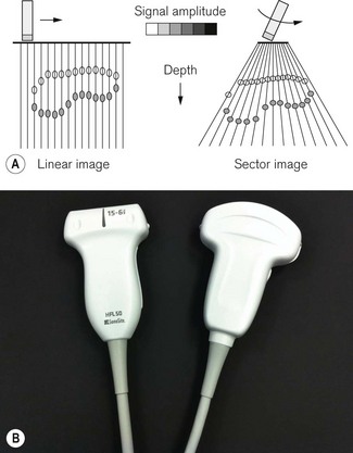
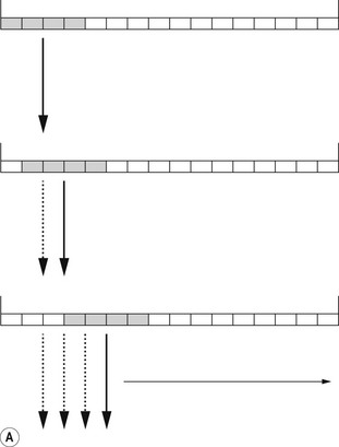
Modern transducer probes consist of an array of 128–256 piezoelectric elements mounted in a flat line to form a linear array, or on a curve to produce a curvilinear array, producing linear and sector images respectively (Fig. 31.5). Groups of elements can be switched electronically between transmit–receive pulse sequences to move the active area along the array. In this way a series of scan lines is produced, scanning through the target to form an image (Fig. 31.6A). The whole image is then scanned and refreshed many times each second to give a continuous real-time image that can show any movement taking place, for example a needle moving towards its intended target.
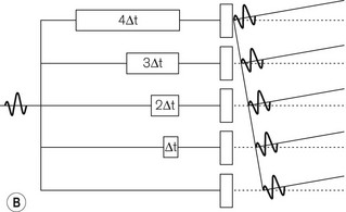
The beam may be steered through different angles by inserting time delays in front of individual elements (Fig. 31.6B). Because the pulse then arrives at adjacent elements at successively later times, the wavefronts of the soundwave propagating away from the elements add up along a line at an angle to the face of the probe. In other words, the transmitted pulse is steered away from a line perpendicular to the probe face. When echoes return to the transducer, the received echoes are again delayed and then added together. Those echoes coming from the steering angle will give a strong signal, as all their wave crests will add together. But for those echoes arriving from other angles, the peaks and troughs will tend to cancel each other out and a signal will not be detected. By switching the time delays electronically, each successive pulse can be steered at a different angle to produce a sector-shaped image. This is the basis for the function of phased array probes, commonly used for cardiac studies and for some intra cavitary applications.
The ultrasound journey
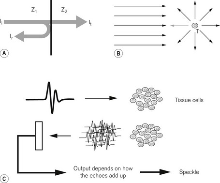
As the ultrasound pulse travels through the body it interacts with the tissue in various ways (Fig. 31.7). At large smooth interfaces, such as are found between one organ and another, muscle–liver for example, some of the energy in the pulse is reflected back towards the transducer as an echo (Fig. 31.7A). This type of reflection from a large smooth interface is known as specular reflection from the Latin speculum meaning a mirror. The strength of the echo will depend on the speed of sound (c) and density (ρ) of the tissues on either side of the interface through a property known as characteristic acoustic impedance (z0). Ii is the incident intensity and Ir is the reflected intensity of ultrasound (Table 31.2).
| Soft tissue–soft tissue | ~1% |
| Soft tissue–air | 99.9% |
| Soft tissue–bone | ~50% |

In practice this means that in going from one soft tissue to another, e.g. muscle–fat, where the density and speed of sound are very similar, only ~1% of the sound energy in the pulse is reflected back to the transducer. The rest of the pulse energy is transmitted on to deeper tissues. In going from soft tissue to a gas there is a very big difference in acoustic impedance between the two. Gas has a very low density and low speed of sound compared with soft tissue. In this case 99.9% of the sound energy is reflected back at the first tissue–gas interface and no ultrasound is transmitted to deeper tissues. The image will show a very bright reflection with no information beyond it. This is also the reason why it is necessary to put gel on the skin of the patient, to exclude all air between the transducer probe and skin so that the ultrasound propagates into the body. For bone, about 50% of the sound energy is reflected at a soft tissue–bone interface giving bone a bright reflection on the image. However, very little is seen beyond the first bone surface as any sound energy that is transmitted into the bone is quickly absorbed.
Speckle
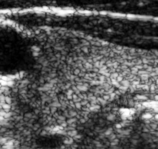
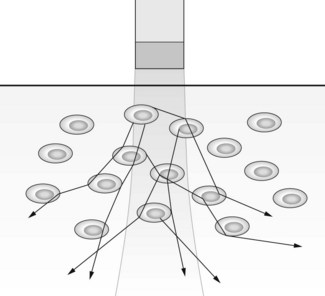
In between the discrete layers of different tissue types the pulse passes through tissue parenchyma. This consists of the cellular structure of the tissue within each organ, together with other microscopic structures that are smaller than the wavelength of the ultrasound. Recall that for the megahertz frequencies of sound used for diagnostic imaging the wavelength is 0.5–0.1 mm. When a sound wave encounters reflectors that are small compared with its wavelength, the sound is scattered in all directions in a process known as Rayleigh scattering (see also Chapter 15, Rayleigh scatter) (Fig. 31.7B). The amount and direction of scattering is strongly dependent on the size of the scatterer and the wavelength or frequency of the sound wave. The transducer will only ‘see’ the very small amount of sound energy scattered in the direction of the transducer. The rest of the energy scattered in other directions is wasted and contributes nothing to the image. The echoes received from scattering form the image we see of tissue parenchyma. However, what we see on the image is not a true image of the microscopic structure of the tissue, as this is too small to resolve. Instead, what we see is a speckle pattern whose appearance depends on the underlying structure of the tissue. Many small scatterers will be within the ultrasound pulse at the same time (Fig. 31.7C). They all send back their tiny echoes at once and what the transducer picks up depends on how the peaks and troughs of all the small sound waves add up. If many peaks arrive at the same time they add up to a large signal and a bright spot will be seen on the image. If the peaks and troughs arrive so that on average they cancel each other out, a small signal will be picked up and a dark spot will be seen on the image. This process is known as superposition of the wavefronts. The image of the tissue parenchyma will, therefore, consist of a random ordering of bright, dark and mid-grey spots forming a speckle pattern (Fig. 31.8). The underlying tissue structure will affect what is seen, so liver speckle looks different from thyroid, and metastases are different from normal tissue, but nevertheless it is important to realize that it is a speckle pattern that is seen, not the microscopic structure of the tissue.
Attenuation
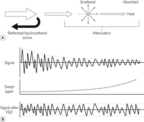
As the ultrasound pulse travels through the body some energy is reflected at interfaces as specular reflection, some is scattered by Rayleigh scattering at microscopic interfaces and some energy is absorbed as heat energy. Heat is simply the energy deposited in the tissue causing increased molecular vibration. All of these mechanisms contribute to attenuation of the pulse as it goes deeper into the body (Fig. 31.9A). We may put in a large amplitude pulse of ultrasound at the skin, but as it passes through tissue the pulse and the echoes reflected back get weaker and weaker. The signals are attenuated until at some depth there is no pulse left to send back echoes. This forms a limit to the penetration of a particular ultrasound transducer. Like scattering, absorption and heating also increases with increasing frequency, so high-frequency probes have poorer penetration than low-frequency probes.
Time gain compensation
Attenuation of the ultrasound pulse has another important consequence for imaging. If strong echoes near the surface get weaker at greater depths, the image should be brighter near the skin surface and get dimmer at greater depths. This would be no good for looking at large uniform organs such as the liver where we want to see the whole organ as uniformly bright (Fig. 31.9B).
In order to overcome this problem the ultrasound scanner applies a gradually increasing gain to the received signal from each transmitted pulse. By this means the decrease in signal strength from echoes arriving later in time, from greater depths, is compensated for by amplifying the signal more. This technique is known as time gain compensation (TGC) or depth gain compensation. It does not increase the penetration of the ultrasound probe for when attenuation has extinguished the pulse, there are no more echoes returning. However, it does enable the image over the useful depth to be uniformly displayed. Beyond the penetration depth only amplified noise will be displayed on the image. TGC is a control that must be correctly adjusted by the user to ensure information in the image is not missed or misinterpreted. Most scanners apply a basic TGC which the user can further adjust. On larger machines the TGC control is usually in the form of sliders set to control the image brightness at 1 cm steps in depth. On portable scanners the control is often simplified to a near field and a far field gain. There is also an overall B-mode gain control affecting the whole image. This should be adjusted so that the brightest parts of the image just reach peak white (Fig. 31.10).
Poor visualization
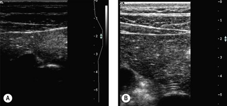
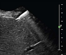
In some patients the image will appear somewhat murky and poorly defined and may be described as poor visualization. This is a result of some types of body fat distorting what should be a well-defined ultrasound beam (Fig. 31.11). Fat consisting of slightly more dense fat globules in a matrix of less dense fat has the same effect on an ultrasound beam as the distorting glass used in bathroom windows has on light. It depends on the particular patient and when seen there is little the operator can do. Pressing the transducer harder on the skin or trying an alternative line of approach to the target may help, but in the end it is one of the limitations of ultrasound as an imaging modality.
Resolution
Axial resolution (Fig. 31.12A) depends on the length of the pulse travelling out along the ultrasound beam. If two targets along the beam axis are just within the pulse at the same time, the echo sent back to the transducer from one target will just overlap the other. In order to see the two targets separately they must be at least half a pulse length apart. The pulse length is nλ, where n is the number of cycles in the pulse and λ the wavelength of ultrasound. A typical transmitted pulse is three cycles long. This gives a pulse length of 0.45 mm at 10 MHz and, therefore, an axial resolution of 0.23 mm. In order to improve the resolution it is necessary to use a shorter pulse or a higher frequency giving a shorter wavelength.
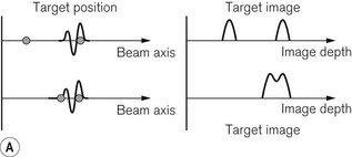
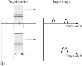
Lateral resolution (Fig. 31.12B) is the resolution in the direction across the beam width, i.e. orthogonal (at right angles) to the axial resolution. As the ultrasound beam is scanned across a target it will just be separated from an adjacent target if the adjacent target is just leaving the beam as the first target is entering the beam. They will be seen as two separate targets on the image if they are more than half a beam width apart. Beam width also depends on frequency with a narrow beam being produced by a higher frequency for a given aperture or active area on the transducer array. For a 10 MHz probe lateral resolution will be slightly greater than the axial resolution at 0.4 mm. From this discussion it may be seen that both the axial and lateral resolutions are improved at higher frequencies, hence the desire to use high-frequency probes.
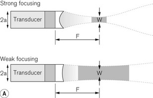
The lateral resolution can be further improved if a lens is put in the ultrasound beam to focus it in a similar way to putting a lens in front of a torch to focus its light (Fig. 31.13A):

Electronic focusing
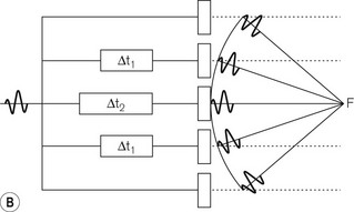
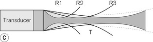
An ultrasound beam will be focused if all of the wavefronts in the sound wave converge on a single point in space: the focal point. This may be achieved by a lens, which refracts or bends the wavefronts into such a converging wave. When a transducer array is used, as is the case in medical imaging, focusing can be achieved electronically by the use of time delays, in a similar manner to electronic beam steering (Fig. 31.13B). Time delays are chosen to control when the transmitted pulse reaches each element so that the propagating wavefront forms a converging line along a circle centred on the desired focal point in front of the transducer. As with the previously described beam steering, the peaks and troughs of the received echoes will add up strongly for echoes arising from the beam directed toward the focal point, but tend to cancel for other directions. By changing the time delays, it is possible to focus the beam on different depths in the tissue. The time delays can be rapidly switched from one set to another so that multiple focal zones can be used in receive, improving the resolution at all depths (Fig. 31.13C). That is, for each transmitted pulse, as echoes arrive from successively greater depths, the next set of time delays is switched in order to focus at that depth. For the transmitted pulse itself, only one focal zone can be used, as that focused pulse travels out to all depths of tissue before it is fully attenuated. Once the pulse has left the transducer, nothing further can be done to change its shape or direction.
Slice thickness
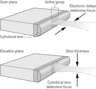
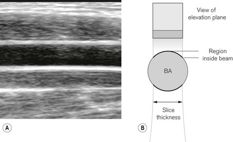
When viewing an ultrasound image we see a slice through the body (Fig. 31.14). The slice in the body is called the scan plane or image plane. It is important to note that the scan plane slice is not infinitesimally thin. The ultrasound beam has a significant width in the out-of-plane or elevation direction. This may be 2–3 mm for a 10 Mhz transducer. This is known as slice thickness and tissue that is outside the image plane, but still within the elevation plane beam width, will also send echoes back to the transducer. This contributes to some degradation in the sharpness of image. It is minimized by the manufacturer putting a weak cylindrical lens across the front of the transducer probe to give some mild focusing in the elevation plane direction.
Artefacts
Post cystic enhancement (Fig. 31.15)
Clear fluids are poor scatterers of ultrasound and there is very little attenuation of the ultrasound as it travels through them. They therefore appear black on the ultrasound image. However, the TGC is operating on the basis that the ultrasound is being attenuated as it travels through tissue. The consequence is that behind the fluid-filled structure, the image is brighter than it should be because the gain has been increased, but the attenuation has not taken place. This effect is known as post cystic enhancement and, together with the dark image of the fluid, is confirmation that the structure seen in the image is fluid filled, such as a cyst, a blood vessel or other fluid collection.
Reverberation (Fig. 31.15)
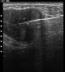
Multiple reflections may also occur within a single target. This will be the case if a hard solid target starts to ring like a bell when it is hit by an ultrasound pulse. The effect is seen on the image as a bright streak or comma behind the target along the beam axis. This is a useful method to detect foreign bodies in tissue and to spot where a needle is, from the reverberation comma seen (Fig. 31.16).
Refraction (Fig. 31.19)
Throughout the image forming process in soft tissue, the assumption is made that the speed of sound is constant at 1540 m s−1. The fact that the speed of sound in real tissue varies by a small amount between the different tissue types gives rise to refraction artefacts. When the ultrasound beam crosses a surface obliquely, the difference in speed of sound either side of the interface causes the beam to be bent, leading to distortion in the image. This is the same effect as seen optically when a pencil is put into a glass of water and viewed from the side. The pencil appears to bend at the air–water interface due to the difference in the speed of light in air and water. Any distortion caused in an ultrasound image is not usually noticed, but when a straight needle is put into tissue and viewed with ultrasound, the needle may appear to be bent as it passes through different tissue layers.
Viewing anatomical structures
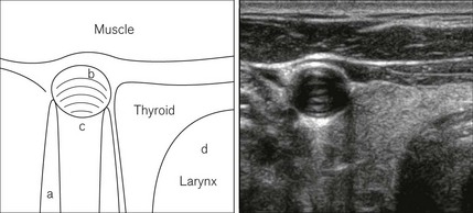
In order to produce a bright sharp surface of an anatomical structure in an image, it is necessary to angle the ultrasound probe so that the ultrasound beams insonate the surface of that structure at 90° (Fig. 31.18). As the surface curves away from the perpendicular it becomes less distinct and slice thickness, reflection and shadowing artefacts become more apparent. Hence if a blood vessel is viewed in longitudinal section, when the image of the walls is sharp and bright, the ultrasound beam is being directed through the centre-line of the vessel. Knowing this can aid ultrasound-directed insertion of needles and cannulas. The easiest way to obtain this longitudinal view is to image the vessel in cross-section with the vessel in the centre of the field of view. Then rotate the probe into the longitudinal view keeping the vessel at the centre of the image as you do so.
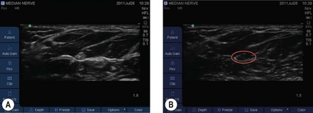
Some tissues have a particular orientation of their structural components causing the ultrasound appearance to vary, depending on the orientation of the image. Their ultrasound appearance is then said to be anisotropic. For example, anisotropy is seen in muscle which has a very strongly striated appearance when viewed along the muscle fibres, but a more uniform appearance when viewed across the fibres. Tendons and nerves also show anisotropy, this being more pronounced in tendons. The effect can be to make the target difficult to see if the probe orientation is not ideal (Fig. 31.20).
Compound mode
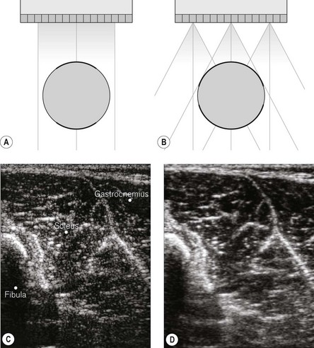
Some scanners have a CT or compound scanning mode that may be turned on or off by the user (Fig. 31.21). This mode sends ultrasound beams into the body at several angles to the face of the transducer from across the whole width of the probe. The effect of this is to insonate each target from a range of angles so reducing the effect of shadowing by sending beams in behind the obstacle, and showing the curved surface of rounded structures more uniformly as the surface is seen by a beam insonating it perpendicularly at more points. Use of compound mode may reduce frame rate and give some blurring of edges due to misregistration of images from multiple directions.
Harmonic imaging
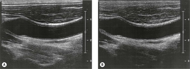
Some scanners have a harmonic imaging mode that the user can switch on or off (Fig. 31.22). This mode reduces the effects of some artefacts, lessening what is often called clutter in the image, and gives some improvement in resolution. It uses the fact that as an ultrasound pulse travels through tissue it changes shape in a way analogous to a wave on the seashore changing its shape as it begins to break. The peaks become more pointed compared with the troughs. What is happening is that some of the energy of the pulse is going into a higher frequency at double the fundamental frequency of the pulse wave. So, for example, if the pulse has a fundamental frequency of 4 MHz when it is transmitted, some of the energy moves to a frequency of 8 MHz as the pulse passes through tissue. If the transducer is a wideband transducer, it can detect both 4 MHz and 8 MHz echoes. In harmonic imaging mode a high-pass filter is used so that the higher frequency 8 MHz echoes are detected and the 4 MHz component is removed. This improves the resolution as the imaging frequency is effectively increased. When using harmonic imaging, the penetration is often poorer and image contrast is reduced.
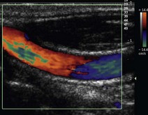
Colour Doppler ultrasound
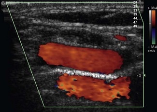
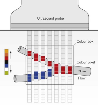
The Doppler effect is very familiar to anyone who has stood at the side of the road and heard a fast police car pass by with its siren going. The Doppler effect is the change in the pitch of the siren heard as the sound waves are squashed together to give a higher frequency as the source comes towards the ‘observer’ and stretched out to give a lower frequency as it moves away. The same effect is used to image moving targets within the body. In particular it is very useful for detecting blood vessels and to aid identification of arteries and veins according to the direction and pulsatility of flow within them. Colour Doppler ultrasound (CDU) uses the difference between the transmitted frequency and the received frequency of the echoes to colour the B-mode image with an overlay, or colour map, showing where there is movement (Fig. 31.23). The difference between received and transmitted frequencies is known as the Doppler frequency. A colour scale with red-yellow for increasing velocity in one direction and blue-green in the other is used. It requires there to be an angle between the blood flow and the ultrasound beam as no Doppler signal will be detected if the vessel is at 90° to the ultrasound beam. The colour map is usually shown within a colour box on the image whose size and angle may be changed, causing angled ultrasound beams to be sent out to avoid the 90° no-signal problem on a given vessel. To confirm direction of flow, it is important to be sure of probe orientation, to know which colour represents flow towards the probe and to know the anatomy being viewed. The angle between blood vessels and the probe can also be improved by tilting the probe on the skin along the line of the array, a process known as heel and toeing.
To form each colour line in the image requires the scanner to send out about 10 pulses, as an estimate of the Doppler frequency is built up from a series of samples, one from each pulse. This has the effect of slowing the image frame rate, as each image takes longer to produce. This may be noticed when scanning in colour mode. In order to keep a high frame rate, the colour box size must be reduced to just include the target of interest. If the blood in the vessel is moving fast, giving a Doppler frequency that is too high to be adequately sampled, an effect known as aliasing is seen. It happens when the pulses are not being sent into the body fast enough to detect the quickly oscillating Doppler frequency. The effect of aliasing is analogous to seeing a wagon wheel or propeller on a movie film going backwards as it gets faster. The repeated rotational motion of the wheel is being inadequately sampled by the frames of the film. In CDU, aliasing is seen as the colour running over the top of the colour scale from yellow to green or vice versa (Fig. 31.24). It can be avoided by increasing the colour scale control. This increases the ultrasound pulse rate thereby increasing the sampling. In a tortuous vessel, the colour filling may alternate red to blue through black as the vessel bends towards and away from the probe. The key to remembering this is: red to blue through black shows a change in flow direction relative to the probe, aliasing with colour over the top shows a high velocity or increased angle of vessel to the probe face (see also Chapter 16, Doppler Effect and equation).