Chapter 4 Physics and Modeling of the Airway
I the Gas Laws
A Ideal Gases
Perhaps the most important law of gas flow in airways is the ideal (or perfect) gas law, which can be written as follows1:
 (1)
(1)P = pressure of gas (pascals or mm Hg)
V = volume of gas (m3 or cm3 or mL)
n = number of moles of the gas in volume V
R = gas constant (8.3143 J g-mol−1·K−1, assuming P in pascals, V in m3)
One mole of gas contains 6.023 × 10²³ molecules, and this quantity is termed Avogadro’s number. One mole of an ideal gas takes up 22.4138 L at standard temperature and pressure (STP); standard temperature is 273.16 K, and standard pressure is 1 atmosphere (760 mm Hg).1 Avogadro also stated that equal volumes of all ideal gases at the same temperature and pressure contain the same number of molecules.
The ideal gas law incorporates the laws of Boyle and Charles.1 Boyle’s law states that, at a constant temperature, the product of pressure and volume (P × V) is equal to a constant. Consequently, P is proportional to 1/V (P ∝ 1/V) at constant T. However, gases do not obey Boyle’s law at temperatures approaching their point of liquefaction (i.e., the point at which the gas becomes a liquid).
Charles’ law states that, at a constant pressure, volume is proportional to temperature (i.e., V ∝ T at constant P). Gay-Lussac’s law states that, at a constant volume, pressure is proportional to temperature (i.e., P ∝ T at constant V).1 Often, these two laws are shortened for convenience to Charles’ law. When a gas obeys both Charles’ law and Boyle’s law, it is said to be an ideal gas and obeys the ideal gas law.
In clinical situations, gases are typically mixtures of several “pure” gases. Quantifiable properties of mixtures may be determined using Dalton’s law of partial pressures. Dalton’s law states that the pressure exerted by a mixture of gases is the sum of the pressures exerted by the individual pure gases1,2:
 (2)
(2)where PA, PB, and PC are the partial pressures of pure ideal gases.
B Nonideal Gases: The van der Waals Effect
Ideal gases have no forces of interaction, but real gases have intermolecular attraction, which requires that the pressure-volume gas law be rewritten as follows1,2:
 (3)
(3)P = pressure of gas (pascals or mm Hg)
V = volume of gas (m3 or cm3 or mL)
n = number of moles of the gas in volume V
R = gas constant (8.3143 J g- mol−1·K−1, assuming P in pascals, V in m3)
The values of a and b for a given gas may be found in physical chemistry textbooks and other sources.1–5 This formulation, provided by van der Waals, accounts for intramolecular forces fairly well.
C Diffusion of Gases
Clinically, diffusion of gases through a membrane is most applicable to gas flow across lung and placental membranes. The most commonly used relation to govern diffusion is Fick’s first law of diffusion, which states that the rate of diffusion of a gas across a barrier is proportional to the concentration gradient for the gas. Fick’s law may be expressed mathematically as follows6:
 (4)
(4)Flux = the number of molecules crossing the membrane each second (molecules/cm2/s)
ΔC = the concentration gradient (molecules/cm3)
Because gases partially dissolve when they come into contact with a liquid, Henry’s law becomes important in some instances. It states that the mass of a gas dissolved in a given amount of liquid is proportional to the pressure of the gas at constant temperature. As a result, the gas concentration (in solvent) is equal to a constant × P (at constant T).1
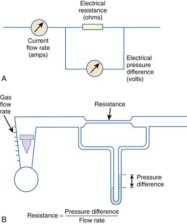
D Pressure, Flow, and Resistance
Flow (i.e., the rate of flow) is equal to the change in pressure (pressure drop or pressure difference) divided by the resistance experienced by the fluid. For example, if the flow is 100 mL/s at a pressure difference of 100 mm Hg, the resistance is 100 mm Hg/100 mL/s, or 1 mm Hg/mL/s. In laminar flow systems only, the resistance is constant, independent of the flow rate.7,8
An important formula that quantifies the relationship of pressure, flow, and resistance in laminar flow systems is given by the Hagen-Poiseuille equation. Poiseuille’s law states that the fluid flow rate through a horizontal straight tube of uniform bore is proportional to the pressure gradient (ΔP), and the fourth power of the radius (π) and is related inversely to the viscosity of the gas (µ, in g/cm·s) and the length of the tube (L, in cm). This law, which is valid for laminar flow only, may be stated as follows7,8:
 (5)
(5)See the discussion of laminar flow in Section II for further details.
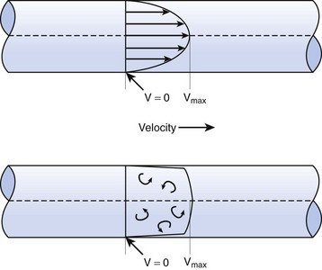
When the flow rate exceeds a critical velocity (the flow velocity below which flow is laminar), the flow loses its laminar parabolic velocity profile, becomes disorderly, and is termed turbulent (Fig. 4-1). If turbulent flow exists, the relationship between pressure drop and flow is no longer governed by the Hagen-Poiseuille equation. Instead, the pressure gradient required (or the resistance encountered) during turbulent flow varies as the square of the flow rate. See the discussion of turbulent flow in Section II.
Viscosity, µ, characterizes the resistance within a fluid to the flow of one layer of molecules over another (shear characteristics).7 Blood viscosity is influenced primarily by hematocrit, so that at low hematocrit blood flow is easier—that is, blood is more dilute. The critical velocity at which turbulent flow begins depends on the ratio of viscosity (µ) to density (ρ), which is defined as the kinematic viscosity (υ)—that is, υ = µ/ρ. (This is illustrated with an example in the section on turbulent flow).7–9 The unit for viscosity is g/cm·s (poise). The typical unit for kinematic viscosity is cm2/s.
The viscosity of water is 0.01 poise at 25° C and 0.007 poise at 37° C. The viscosity of air is 183 micropoise at 18° C. Its density (dry) is 1.213 g/L.10
 (6)
(6)where D0 is a known density of the gas at temperature T0 and pressure P0, and D is the density of the gas at temperature T and pressure P. For dry air at 18° C and 760 mm Hg (atmospheric pressure), D = 1.213 g/L.4
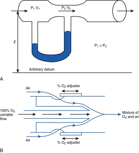
The fall in pressure at points of flow constriction (where the flow velocity is higher) is known as the Bernoulli effect (Fig. 4-2).7,8 This phenomenon is used in apparatus employing the Venturi principle, such as gas nebulizers, Venturi flowmeters, and some oxygen face masks. The lower pressure related to the Bernoulli effect sucks in (entrains) air to mix with oxygen.
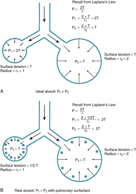
One final consideration that is important in the study of the airway is Laplace’s law for a sphere (Fig. 4-3). It states that, for a sphere with one air-liquid interface (e.g., an alveolus), the relation between the transmural pressure difference, surface tension, and sphere radius is described by the following equation11:
 (7)
(7)E Example: Analysis of Transtracheal Jet Ventilation
Transtracheal jet ventilation (TTJV) has been used to oxygenate and ventilate patients who would otherwise perish because of a lost airway.6 It is a temporizing measure that is used only until an airway can be secured. It is usually employed using equipment commonly available in the operating or emergency room and often using the 50-psi wall oxygen source.6,12–14
1 Analysis
 min = 0.5 L.
In a TTJV setup consisting of a 14-G angiographic catheter connected to a regulated oxygen source by a 4.5-foot polyvinyl chloride (PVC) tube of  -inch inner diameter (ID), for oxygen flows between 10 and 60 L/min, the resistance was found to be relatively constant between 0.6 and 0.8 psi/L/min.15
II Gas Flow
A Laminar Flow
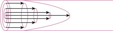
In laminar flow, fluid particles flow along smooth paths in layers, or laminas, with one layer gliding smoothly over an adjacent layer.7 Any tendencies toward instability and turbulence are damped out by viscous shear forces that resist the relative motion of adjacent fluid layers. Under laminar flow conditions through a tube, the flow velocity is greatest at the center of the tube flow and zero at the inner edge of the tube (Fig. 4-4; see also Fig. 4-1). The flow profile has a parabolic shape. Under these conditions in a horizontal tube, the relation between flow, tube, and gas characteristics is given by the Hagen-Poiseuille equation (Equation 5), restated as follows7–9:
 (8)
(8) = flow rate (cm3/s)
Typical units are shown in parentheses. The dot indicates rate of change: V represents volume, and  represents the rate of change of volume, or flow rate. Another way of looking at this concept is that, under conditions of laminar flow through a tube of known radius, the pressure difference across the tube is given by the following proportionality (which is also essentially the same as Equation 5):
 (9)
(9) (10)
(10)B Turbulent Flow
Flow in tubes below the critical flow rate remains mostly laminar. However, at flows greater than the critical flow rate, the flow becomes increasingly turbulent. Under turbulent flow conditions, the parabolic flow pattern is lost, and the resistance to flow increases with flow itself. Turbulence may also be created where sharp angles, changes in diameter, and branches are encountered (Fig. 4-5). The flow-pressure drop relationship is given approximately by the following equation7,8:
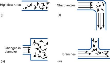
Figure 4-5 Turbulent flow. Four circumstances likely to produce turbulent flow.
(From Nunn JF: Nunn’s applied respiratory physiology, ed 4, Stoneham, MA, 1993, Butterworth-Heinemann.)
 (11)
(11)1 Reynolds Number Calculation Example
The Reynolds number (Re) represents the ratio of inertial forces to viscous forces.7,8,16 It is useful because it characterizes the flow through a long, straight tube of uniform bore. It is a dimensionless number having the following form:
 (12)
(12) = flow rate (mL/s)
Typical units are shown in brackets. For tubes that are long compared with their diameter (i.e., length ÷ diameter > 0.06 × Re),8 the flow is laminar when Re is less than 2000. For shorter tubes, flow is turbulent at Re values as low as 280.
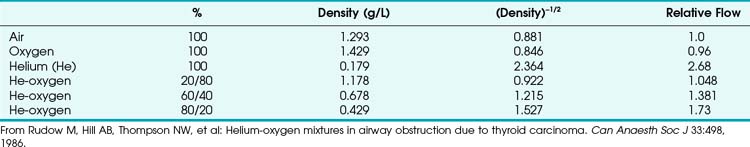
When a tube’s radius exceeds its length, it is an orifice; flow through an orifice is always turbulent. Under these conditions, the flow is influenced by the density rather than the viscosity of the fluid.17 This characteristic explains why heliox (e.g., the mixture of 70% He and 30% O2) flows better in a narrow edematous glottis: as the following data suggest, helium has a very low density and thus presents less resistance to flow through an orifice.
| Viscosity at 20° C | Density at 20° C | |
|---|---|---|
| Helium | 194.1 micropoise | 0.179 g/L |
| Oxygen | 210.8 micropoise | 1.429 g/L |
 ) = 60 L/min = 1000 mL/s
With this information, one can calculate the Reynolds number:
 (13)
(13)Because this number greatly exceeds 2000, flow is probably quite turbulent.
C Critical Velocity
The critical velocity is the point at which the transition from laminar to turbulent flow begins. This point is reached when Re becomes the critical Reynolds number, Recrit. Critical velocity, the flow velocity below which flow is laminar, is calculated by the following equation8:
 (14)
(14) (15)
(15)D Flow Through an Orifice
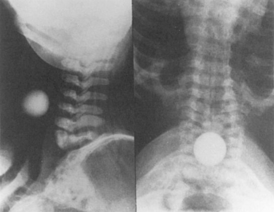
Flow through an orifice (defined as flow through a tube whose length is smaller than its radius) is always somewhat turbulent.17 Clinically, airway-obstructing conditions such as epiglottitis or swallowed obstructions are often best viewed as breathing through an orifice (Fig. 4-6). Under such conditions, the approximate flow across the orifice varies inversely with the square root of the gas density:
 (16)
(16)This is in contrast to laminar flow conditions, in which gas flow varies inversely with gas viscosity. The viscosity values for helium and oxygen are similar, but their densities are very different (Table 4-1). Table 4-2 provides useful data to allow comparison of gas flow rates through an orifice.18
TABLE 4-1 Viscosity and Density Differences of Anesthetic Gases
| Viscosity at 300 K | Density at 20° C | |
|---|---|---|
| Air | 18.6 µPa × s | 1.293 g/L |
| Nitrogen | 17.9 µPa × s | 1.250 g/L |
| Nitrous oxide | 15.0 µPa × s | 1.965 g/L |
| Helium | 20.0 µPa × s | 0.178 g/L |
| Oxygen | 20.8 µPa × s | 1.429 g/L |
Data from Haynes WM: CRC Handbook of chemistry and physics, ed 91, Boca Raton, FL, 2010, CRC Press, and Streeter VL, Wylie EB, Bedford KW: Fluid mechanics, ed 9, New York, 1998, McGraw-Hill.
1 Helium-Oxygen Mixtures
The low density of helium allows it to play a significant clinical role in the management of some forms of airway obstruction.19–22 For instance, Rudow and colleagues described the use of helium-oxygen (heliox) mixtures in a patient with severe airway obstruction related to a large thyroid mass (see next section for clinical examples).18
Although the use of heliox mixtures in patients with upper airway obstruction has met with considerable success, the hope that this approach would also work well for patients with severe asthma has not been borne out. In a systematic review of seven clinical trials involving 392 patients with acute asthma, the authors cautioned that “existing evidence does not provide support for the administration of helium-oxygen mixtures to emergency department patients with moderate-to-severe acute asthma.”23 A similar study noted that “heliox may offer mild-to-moderate benefits in patients with acute asthma within the first hour of use, but its advantages become less apparent beyond 1 hour, as most conventionally treated patients improve to similar levels, with or without it”; however, the authors suggested that its effect “may be more pronounced in more severe cases.” They concluded that “there are insufficient data on whether heliox can avert endotracheal intubation, or change intensive care and hospital admission rates and duration, or mortality.”24
2 Clinical Vignettes
Rudow and colleagues reported the following clinical illustration of heliox therapy.18 A 78-year-old woman with both breast cancer and ophthalmic melanoma developed airway obstruction from a thyroid carcinoma that extended into her mediastinum and compressed her trachea. She had a 2-month history of worsening dyspnea, especially when positioned supine. On examination, inspiratory and expiratory stridor was present. The chest radiograph showed a large superior mediastinal mass and pulmonary metastases. A solid mass was identified on a thyroid ultrasound scan. Computed tomography revealed a large mass at the thoracic inlet and extending caudally. Clinically, the patient was exhausted and in respiratory distress.
Another interesting clinical scenario was published by Khanlou and Eiger.25 They presented the case of a 69-year-old woman in whom bilateral vocal cord paralysis developed after radiation therapy. Heliox was successfully used for temporary management of the resultant upper airway obstruction until the patient was able to receive a tracheostomy.
A final clinical vignette was reported by Polaner,26 who used the laryngeal mask airway and an 80 : 20 heliox mixture to administer anesthesia to a 3-year-old boy with asthma and a large anterior mediastinal mass. Clinical management involved an unusual combination of management strategies: the child was kept in the sitting position, spontaneous ventilation with a halothane-in-heliox inhalation induction was used, and airway stimulation was minimized by use of the laryngeal mask airway. However, the author cautioned that cases such as these can readily take a deadly turn, noting that “one must, of course, always be prepared to intervene with either manipulations of patient position in the event of airway compromise (including upright, lateral, and prone) or more aggressive strategies, such as rigid bronchoscopy and even median sternotomy (in the case of intractable cardiovascular collapse), or to allow the patient to awaken if critical airway or cardiovascular compromise becomes evident at any time during the course of the anesthesia.”26
E Pressure Differences
From the analysis of equations governing laminar flow and turbulent flow, the pressure drop along the noncompliant portion of the airway is given approximately by the Rohrer equation27:
 (17)
(17) is small (i.e., with predominantly laminar flow). However, it is known that under conditions of laminar flow, K1 is largely influenced by viscosity rather than density, and K2 (the turbulent term) is influenced primarily by density and not viscosity.
F Resistance to Gas Flow
When pressure readings are taken at each end of a horizontal tube with a fluid flowing through it, one notices that they are not identical: The pressure at the distal end of the tube is less than the pressure at the proximal end (with fluid flowing from the proximal to the distal end). This pressure loss is attributable to frictional losses incurred by the fluid when in contact with the inside of the tube. This is analogous to heat losses incurred by resistors in an electrical circuit (Fig. 4-7).
Frictional losses are irreversible; that is, the energy lost cannot be recovered by the fluid and is mostly lost as heat. If the tube is not horizontal, there are additional pressure differences attributable to height differences. The most common relation that describes the flow in a tube is the Bernoulli equation, which is valid for both laminar and turbulent flow8:
 (18)
(18)g = gravitational constant (9.81 m/s2 or 9.81 N/kg)
P = pressure (pascals or N/m2)
Typical units are shown in square brackets. Equation 18 is in units of meters and is termed “meters of head loss.” This is typical of fluid mechanics equations. As mentioned previously, the Bernoulli equation is valid for both laminar and turbulent flow.
1 Endotracheal Tube Resistance
ETTs, like all tubes, offer resistance to fluid flow (Fig. 4-8). However, ETTs do not add external resistance to the normal airway; rather, they act as a substitute for the normal resistance of the airway from the mouth to the trachea, which accounts for 30% to 40% of normal airway resistance.28 This is important because, although mechanical ventilators can overcome impedance to inspiratory flow during extended periods of artificial respiration, they do not augment passive exhalation. Resistance to exhalation through a long, small-diameter ETT, which is compounded by turbulence, can seriously constrain ventilation rate and tidal volume.29,30
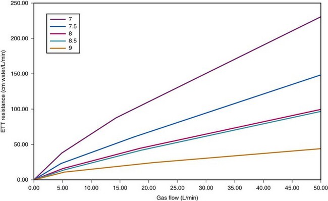
Figure 4-8 Dependence of endotracheal tube (ETT) on flow. The data provided by Hicks in Table 4-3 can be used to show that ETT resistance increases nonlinearly with flow (because of turbulence effects). For pure laminar flow, resistance would be constant, regardless of flow.
The use of the ETT influences respiration in a number of ways. First, it decreases effective airway diameter and therefore increases the resistance to breathing. Resistance is further increased by the curved nature of the tube; resistance measurements are typically about 3% higher than if the tubes were straight.31 Also, the passage from the mouth to the larynx is not a smooth curve and may create additional turbulence. Second, studies show that intubated patients experience decreased peak flow rates (inspiratory and expiratory), decreased forced vital capacity, and decreased forced expiratory volume in 1 second (FEV1).32 However, the tube may paradoxically increase peak flow rates during forced expiration by preventing dynamic compression of the trachea.32 Finally, the tube may cause mechanical irritation of the larynx and trachea that may lead to a reflex constriction of the airway distal to the tube.33
The combination of tube and connector may cause higher resistance than the tube alone. Moreover, because of turbulence at component connections, the total resistance of a system is not necessarily the sum of the resistances of its component parts, especially if sharp-angled connectors are used (see Fig. 4-5).25,34 In addition, humidified gases contribute to slightly higher resistances because of the increased density of moist gas, and the resistance of single-lumen tubes is generally lower than that of double-lumen tubes.35
The resistance associated with ETTs may be reduced by increasing the tube diameter, decreasing tube length, or decreasing the gas density (hence, the occasional use of heliox mixtures). It has been suggested that the presence of an ETT may double the work of breathing in chronically intubated adults and may lead to respiratory failure in some infants.31 Therefore, it is important to use as large an ETT as is practical in patients who exhibit respiratory dysfunction.
ETT resistance can be measured in the laboratory using differential pressure and flow measurement techniques,36,37 most commonly by the method of Gaensler and colleagues.38 Theoretical estimates of resistance under laminar flow conditions can also be obtained by using the Poiseuille equation. In vivo measurements of ETT resistance are generally higher than in vitro measurements, perhaps because of secretions, head or neck position, tube deformation, or increased turbulence.10,39
Airway resistance may be established from first principles using Poiseuille’s law if the gas flow is laminar. If gas flow is turbulent, resistance is no longer independent of material properties, and empirical measurements become the only feasible means of characterizing resistance. Intrinsic airway resistance is determined by measuring the transairway pressure—that is, the pressure drop between the airway opening and the alveoli. The following relationship applies40:
 (19)
(19)R = airway resistance (cm H2O/L/s)
Pairway = proximal airway pressure (cm H2O)
 = gas flow rate (L/s)
Typical units used are shown in parentheses.
In clinical practice, airway resistance is most easily determined by using a whole-body plethysmograph. However, this apparatus is unsuitable for critically ill patients. An alternative method of presenting airway resistance was provided by Hicks,40 who used the following equation and constants:
 (20)
(20) = gas flow (L/min)
The values for the coefficients a and b depend on tube size and are provided in Table 4-3.
| Tube | a | b |
|---|---|---|
| 7.0 | 9.78 | 1.81 |
| 7.5 | 7.73 | 1.75 |
| 8.0 | 5.90 | 1.72 |
| 8.5 | 4.61 | 1.78 |
| 9.0 | 3.90 | 1.63 |
From Hicks GH: Monitoring respiratory mechanics. Probl Respir Care 2:191, 1989.
Figure 4-8 depicts the effects of tube diameter and flow rate on ETT resistance. Notice that resistance is increased as a result of increasing turbulence caused by decreasing ETT diameter and increasing flow rate.
Clinically, the issue of ETT resistance is perhaps most important in pediatrics and during T-piece trials. In a laboratory study, Manczur and coworkers sought to determine the resistances of ETTs commonly used in neonatal and pediatric intensive care units.41 They examined straight tubes with IDs of 2.5 to 6 mm and shouldered (Cole) tubes with ratios of ID to outer diameter ranging from 2.5/4 to 3.5/5 mm. Predictably, they found that resistance increased as ETT diameter decreased. The resistances of the 6-mm ID ETTs were 3.1 and 4.6 cm H2O/L/s at flows of 5 and 10 L/min, respectively, and the resistances of the 2.5-mm ID ETT were 81.2 and 139.4 cm H2O/L/s, respectively. The authors reported that shortening an ETT to a length appropriate for the patient (e.g., shortening a 4.0-mm ID ETT from 20.7 to 11.3 cm) reduced resistance on average by 22%. They also noted that the resistance of a Cole tube was “about 50% lower than that of a straight tube with an ID corresponding to the narrow part of the shouldered tube.”
Using an acoustic reflection research method, Straus and associates sought to study the influence of ETT resistance during T-piece trials by comparing the work of breathing in 14 successfully extubated patients at the end of a 2-hour trial and after extubation.42 They found that work of breathing was identical in both groups and there was no significant difference between the beginning and the end of the T-piece trial. The work caused by the ETT amounted to about 11.0% of the total work of breathing, and the supralaryngeal airway resistance was significantly smaller than the ETT resistance. The authors concluded that “a 2 hr trial of spontaneous breathing through an ETT well mimics the work of breathing performed after extubation, in patients who pass a weaning trial and do not require reintubation.”
III Work of Breathing
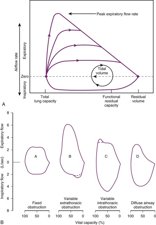
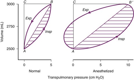
Breathing comprises a two-part cycle: inspiration and expiration. During normal breathing, inspiration is an active, energy-consuming process, and expiration is ordinarily a passive process in which the diaphragm and intercostal muscles relax (Figs. 4-9 and 4-10). However, expiration becomes an active process during forced expiration, such as during exercise or during expiration against a resistance load. Several studies have examined the work of breathing in various clinical settings.43–48
Considering only normal breathing, the work of breathing is given by the following formulas:
Because the air pressure in the lung varies with lung volume and pressure measurements are obtained distal to the end of the ETT, work may be expressed as follows49:
 (21)
(21)dV = (infinitesimal) volume of gas added to the lung (mL)
When the pressure varies as a function of time, Equation 21 may be integrated in the following manner:
 (22)
(22)Changing the limits of integration yields the following:
 (23)
(23)t1 = time at the beginning of inspiration (s)
t2 = time at the end of inspiration (s)
P = pressure measured at a point of interest in the airway (e.g., at the tip of the ETT or at the carina) (cm H2O)
 = flow (mL/s)
 (24)
(24) (25)
(25)where ΔP is the pressure drop across the tube.
Often, the pressure gradient ΔP is relatively constant during inspiration, and therefore:
 (26)
(26)The total work done, measured in joules (kg × m2/s2), is as follows:
 (27)
(27)IV Pulmonary Biomechanics
A The Respiratory Mechanics Equation
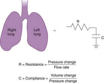
Approximately 3% of the body’s total energy is required to maintain normal respiratory function.11 Energy is required to overcome three main forces: (1) the elastic resistance of the lungs, which restores the lungs to their original size after inflation; (2) the force required to move the rib cage, diaphragm, and appropriate visceral contents; and (3) the dissipative resistance of the airway and any breathing apparatus.50 The respiratory system is commonly modeled as the frictional airway RL that is in series with the lung compliance CL. Such a model is analogous to a resistor and capacitor in series that form a resistive-capacitive (RC) circuit (Fig. 4-11).
A transmural (PTM) pressure gradient exists between the airway at the mouth (i.e., at atmospheric pressure) and the pressure inside the pleural cavity. This pressure gradient is responsible for the lungs’ “hugging” the thoracic cavity as the chest enlarges during inspiration. The presence of an external breathing apparatus causes a further pressure loss (PEXT). The total pressure drop between the atmosphere and the pleural cavity is given by the respiratory mechanics equation and may be modeled as follows50:
 (28)
(28) (29)
(29) (30)
(30)PTOTAL = pressure drop between atmosphere and pleural cavity
PEXT = pressure drop across external breathing apparatus
PTM = transmural pressure gradient
REXT = external apparatus resistance (e.g., an ETT)
 = dV/dt = gas flow rate into the lungs
V = volume of gas above the functional residual capacity (FRC) in the lungs
1 The Pulmonary Time Constant
Using the previous formula (Equation 29) in the case that no external resistance exists, one can show that, during passive expiration, the volume in the lungs in excess of FRC takes on the following form51:
 (31)
(31)where V0 is the volume taken in during inspiration and τ = RLCL is the time constant for the lungs.
Flow from the lungs is obtained by differentiating this equation with respect to time:
 (32)
(32)Tau (τ) may be now estimated by dividing the preceding equation by the first one:
 (33)
(33) ) against volume (V) during expiration. Another means of estimating τ is by taking the natural logarithm of the volume equation V = V0e−t/τ.
 (34)
(34)2 Determination of Rohrer’s Constants
A more complete approach to modeling the pressure-flow relationship of the respiratory system assumes that a single time constant τ may be inadequate to describe pulmonary biomechanics in some situations. The classical form of the equation,27
 (35)
(35)can be changed to a more elaborate form of:
 (36)
(36)where K1 and K2 are known as Rohrer’s constants and (K1 + K2) is a form of RL.
 (37)
(37)When this equation is expressed in the following form,
 (38)
(38)K1 and K2 may be determined as the intercept and slope, respectively, of a plot of V/CL against
  .
.
3 Compliance
Pulmonary compliance measurements reflect the elastic properties of the lungs and thorax and are influenced by factors such as degree of muscular tension, degree of interstitial lung water, degree of pulmonary fibrosis, degree of lung inflation, and alveolar surface tension.52 Total respiratory system compliance is given by the following calculation40:
 (39)
(39) (40)
(40)The values shown in parentheses are some typical normal adult values that can be used for modeling purposes.40 Elastance, the reciprocal of compliance, offers notational advantage over compliance in some physiologic problems. However, its use has not been popular in clinical practice.
Compliance may be estimated using the pulmonary time constant, τ. If a linear resistance of known value (ΔR) is added to the patient’s airway, the time constant will change to τ′, as follows27:
 (41)
(41) (42)
(42)B An Advanced Formulation of the Respiratory Mechanics Equation
An alternative to the elementary respiratory mechanics equation may be used to describe the physical behavior of the lungs. The original formulation of this advanced respiratory mechanics equation was carried out by Rohrer during World War I, but the first completely correct formulation was devised by Gaensler and colleagues and has the following form38:
 (43)
(43) = gas flow rate into (out of) lung
 term is very important in accurately quantifying the pressure losses of respiration. In addition, the advanced equation combines the resistance losses into the constants K1 and K2, which require only empirical determination.
V Anesthesia at Moderate Altitude
The approximate alveolar gas equation is a useful tool in quantifying the differences that occur at higher elevations53:
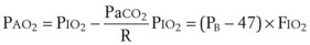 (44)
(44)PAO2 = alveolar oxygen tension
PIO2 = inspired oxygen tension partial pressure
PaCO2 = arterial carbon dioxide tension
R = 0.8 → gas exchange coefficient (CO2 produced/O2 consumed)
PB = barometric pressure (760 mm Hg at sea level)
47 = water vapor pressure at 37° C
FIO2 = fraction of inspired oxygen = 0.21 at all altitudes (room air)
All tensions are in mm Hg (torr).
A Altered Partial Pressure of Gases
The effect of altitude is very apparent on the partial pressure of administered gases. The partial pressure of oxygen is given by PIO2 = (PB − PH2O) × 0.21. At 1524 m (5000 ft) above sea level, PIO2 is reduced to 128 mm Hg from 158 mm Hg at sea level, so that the maximum PaO2 is about 83 mm Hg (assuming PaCO2 = 36).54 At 3048 m (10,000 ft), PIO2 is 111 mm Hg, and the maximum PaO2 is 65 mm Hg.54 In order to counteract the effects of the hypoxia, ventilation is increased, so that at 5000 ft PaCO2 = 36 mm Hg, and at 3048 m PaCO2 = 34 mm Hg on average.54 The effectiveness of nitrous oxide (N2O) decreases with altitude because of an absolute reduction of its partial pressure (tension).
 (45)
(45)F Flowmeter Calibration
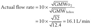
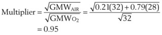
The calibration of standard flowmeters, such as the Thorpe tube, depends on gas properties. Usually, a particular flowmeter is calibrated for a particular gas, such as oxygen or air. The factor used to convert nominal flow measurements to actual flow measurements is given by the following equation53:
 (46)
(46)A list of common anesthetic gases and their respective GMWs is presented in Table 4-4.
TABLE 4-4 Gram Molecular Weight (GMW) for Some Common and Anesthetic Gases
| Name | Symbol | GMW |
|---|---|---|
| Hydrogen | H | 1.00797 |
| Helium | He | 4.0026 |
| Nitrogen (molecular) | N2 | 28.0134 |
| Oxygen (molecular) | O2 | 31.9988 |
| Neon | Ne | 20.183 |
| Argon | Ar | 39.948 |
| Xenon | Xe | 131.30 |
| Halothane | CF3CClBrH | 197 |
| Isoflurane | CF2H-O-CHClCF3 | 184.5 |
| Enflurane | CF2H-O-CF2CFHCl | 184.5 |
| Nitrous oxide | N2O | 44.013 |
 (47)
(47) (48)
(48) (49)
(49) (50)
(50)G Anesthetic Implications
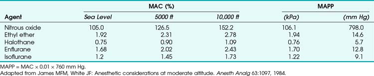
At 10,000 ft, a 30% O2 mixture has the same partial pressure as a 20% O2 mixture at sea level.54 In addition, the reduction in partial pressure of N2O that occurs seriously impairs the effectiveness of the agent, and its administration may be of no benefit. The concept of minimum alveolar concentration (MAC) does not apply at higher altitudes and should be replaced by the concept of minimal alveolar partial pressure (MAPP) (Table 4-5). The use of this concept would eliminate many of the problems identified earlier.
VI Estimation of Gas Rates
A Estimation of Carbon Dioxide Production Rate
 ) of a patient may be estimated in the following manner. The CO2 production rate can be described as the product of the amount of CO2 produced per breath and the number of breaths per minute (BPM), with typical units of mL/min. Therefore,
  may be expressed as follows:
 (51)
(51) (52)
(52)The amount of CO2 produced per breath is calculated as follows:
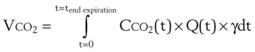 (53)
(53)B Estimation of Oxygen Consumption Rate
 . The oxygen consumption rate can be expressed as the product of oxygen consumed per breath and the number of breaths per minute. Mathematically, this may be written as follows:
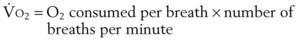 (54)
(54) (55)
(55)The amount of O2 consumed per breath can now be expressed as follows:
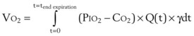 (56)
(56) and
and  are linked by the respiratory exchange coefficient RQ (RQ =
  ), which is governed largely by diet; some diets produce less CO2 than others and have a smaller RQ). Typically, RQ = 0.8.
  and
and  both go up with increases in metabolism, which may be related to factors such as fever, sepsis, light anesthesia, shivering, malignant hyperthermia, and thyroid storm. Decreases in
  and
and  may also have many causes (e.g., hypothermia, deep anesthesia, hypothyroidism).
VII Mathematical Modeling Related to the Airway
B Background
Some physiologic systems are especially well suited to physiologic modeling. For example, physiologic modeling of the cardiopulmonary system may be performed to examine issues such as the determinants of pulmonary gas exchange. For instance, both Doyle and Viale and their coauthors have written custom software to explore the determinants of the arterial-alveolar oxygen tension ratio, and Torda has explored the determinants of the alveolar-arterial oxygen tension difference in a similar manner.55–57 Before the common use of digital computers, graphic techniques were sometimes used for solving respiratory physiologic models. A well-known example is the early work by Kelman and colleagues on the influence of cardiac output (CO) on arterial oxygenation.58 Central to the construction of such a mathematical model is the existence of a number of equations relating physiologic parameters. Examples of physiologic relationships in the respiratory system that are well described by equations include (1) the alveolar gas equation,53,59 (2) the pulmonary shunt equation,60 (3) the blood oxygen content equation,60 and (4) various equations describing the oxyhemoglobin dissociation curve.61–65
C Problems in Model Solving
Some authors have applied successive approximation methods with custom-written software to solve equation sets of this kind.55 However, this approach may involve considerable effort, even by experienced computer programmers. Furthermore, many physiologists have limited experience and training in writing computer programs. The next section describes how equation-solving computer programs can be used to advantage to solve complex physiologic modeling equations. TK SOLVER (Universal Technical Systems, Inc., Rockford, IL) is the equation-solver package used in most of the examples given here, but many other packages could also have been used.
D Description of TK SOLVER
TK SOLVER (the TK stands for “tool kit”) is a software package for equation solving.2,26,47,66,67 Although intended primarily for engineering applications, TK SOLVER functions well in a variety of other application areas. On start-up, TK SOLVER displays 2 “sheets” or tables out of a total of 13. The Variable Sheet is presented on the bottom “window,” and the Rule Sheet goes on the top. Equations are entered in the Rule Sheet using a built-in editor; the variables associated with the equations are then automatically entered in the variable sheet by TK SOLVER. Errors such as unmatched parentheses are automatically detected. Figure 4-12 shows sample Rule and Variable Sheets for a pulmonary exchange model.
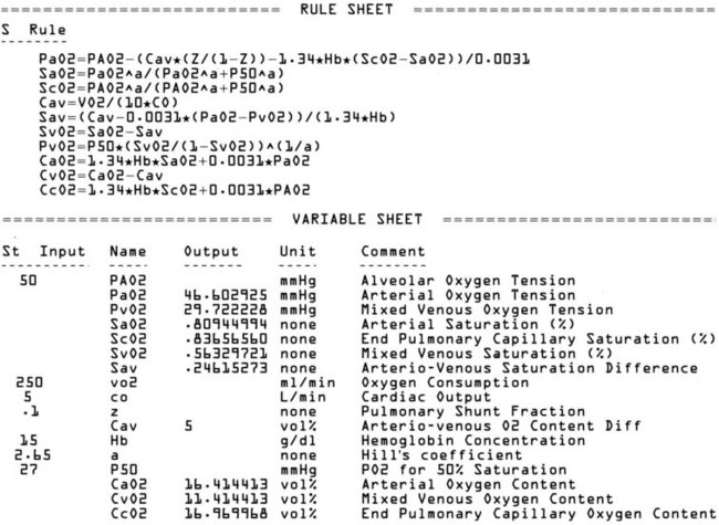
Figure 4-12 Sample TK SOLVER Rule Sheet (top) and Variable Sheet (bottom). In this case, equations relate factors that determine arterial oxygen tension (PaO2). All variables are defined in comment section of variable sheet. The first equation in the Rule Sheet is from Torda and Doyle.55,57 The second and third equations are from Hill.64
Once the equations are entered, TK SOLVER is ready to find solutions. In some cases, the equation set can be solved in “direct-solver” mode, but complex equation sets usually must be solved in “iterative-solver” mode on the basis of initial guesses for all variables. A discussion of the methods used to obtain solutions has been presented by Konopasek and Jayaraman.68 A book reviewing TK SOLVER from a user’s viewpoint is also available.69
E Example 1: Application of Mathematical Modeling to the Study of Gas Exchange Indices
1. Alveolar-arterial oxygen tension difference (PAO2 − PaO2)57,69–71
2. Arterial-alveolar oxygen tension ratio (PaO2/PAO2)55,56,72–74
The importance of these indices and the controversies surrounding their clinical application are reflected in the many publications concerning their use and limitations.34,66,77–79
1 Analysis
 (57)
(57) = mixed venous oxygen content
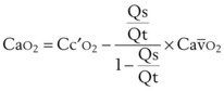
By algebraic manipulation of the shunt equation, it is possible to relate arterial oxygen tension to its influencing factors55,57:
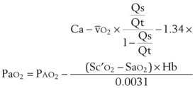 (58)
(58) (vol%) is the arterial–mixed venous oxygen content difference (= Ca
 ), Sc′
 (59)
(59)Equation 58 does not explicitly show the influence of P50 (the oxygen tension corresponding to 50% hemoglobin saturation) on arterial oxygen tension; such influences are mediated indirectly, principally through the SaO2 term. To make explicit the influence of PaO2 and P50 on SaO2, we use the relationship given by Hill’s equation64:
 (60)
(60)where n is an empirical constant (usually taken as 2.65).
A similar expression relates PAO2, P50, and Sc′O2.
The arterial oxygen tension (PaO2), the alveolar-arterial oxygen tension difference (PAO2 − PaO2), and the arterial-alveolar oxygen tension ratio (PaO2/PAO2) can then be obtained using Equations 58, 59, and 60 for specific choices of physiologic variables. Unfortunately, Equation 58 is not easily solved because it requires the solution of two simultaneous nonlinear equations (i.e., equations 58 and 60). In the past, a custom, computer-based successive approximation method was employed to obtain a solution. This amounted to iteratively making successively more accurate estimates of PaO2 levels that satisfied both of those equations. In the case of Doyle,55 Equation 58 was solved in this way to an accuracy of 0.1 mm Hg for various values of Hb,  , FIO2, PaCO2, and Qs/Qt. The process is considerably simplified when TK SOLVER is used, as can be seen by examining the equation sheets presented in Figure 4-12.
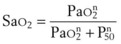
F Example 2: Theoretical Study of Hemoglobin Concentration Effects on Gas Exchange Indices
It is of both theoretical and clinical interest to know what changes in gas exchange indices might be expected with changes in Hb when other physiologic parameters are kept constant. Figure 4-13 shows the results of varying Hb under the following conditions:
 ) = 250 mL/min
G Example 3: Modeling the Oxygenation Effects of P50 Changes at Altitude
It is well known that the oxyhemoglobin dissociation curve shifts in response to physiologic changes. Acidosis, hypercarbia, increased temperature, and increased levels of 2,3-diphosphoglycerate (2,3-DPG) all shift the curve to the right, reducing the affinity of hemoglobin for oxygen and thereby facilitating release of oxygen into tissues. Patients with chronic anemia, for example, have increased intraerythrocyte levels of 2,3-DPG and a right-shifted oxyhemoglobin curve.80 Teleologically, this would also appear to be an appropriate response to high-altitude hypoxemia, but in fact the opposite is true: Animals that have successfully adapted to high-altitude hypoxemia have left-shifted curves,81–83 as do Sherpas.82,84 In the example that follows, computer modeling is used to develop a possible explanation for this finding.
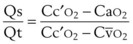
It can be theorized that a left-shifted curve is beneficial in high-altitude hypoxemia because it increases arterial oxygen content by virtue of increasing pulmonary end-capillary oxygen content. The shunt equation described earlier (Equation 57) can be rearranged as follows:
 (61)
(61) (62)
(62)PAO2 is determined only by the alveolar gas equation and is independent of the position of the oxyhemoglobin curve.60 Therefore, the dissolved oxygen portion of Cc′O2 is also independent of the curve position. However, the Sc′O2 term does vary with curve position, increasing with a left-shifted curve. Therefore, Cc′O2 also increases with a left shift, taking on a maximum value of
 (63)
(63)We now consider the effects of P50 changes in two situations.
1. In Situation A, a patient has high-altitude hypoxemia as a result of a PAO2 of 50 mm Hg. With a CO of 5 L/min, an Hb of 15 g/dL, oxygen consumption ( ) of 250 mL/min, and a shunt fraction (Qs/Qt) of 0.1, it can be shown (Table 4-6) that CaO2 changes from 16.41 vol% with a P50 of 27 mm Hg to 18.44 vol% with a P50 of 18 mm Hg—a significant increase.
2. In Situation B, a patient has a large pulmonary shunt (Qs/Qt = 0.4), a normal PAO2 (100 mm Hg), and other parameters as in situation A. In this case, CaO2 goes from 16.47 vol% with a P50 of 27 mm Hg to 16.87 vol% with a P50 of 18 mm Hg—an insignificant change (see Table 4-6).
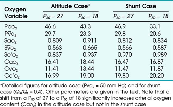
Figure 4-14 illustrates this concept in more detail, showing the two examples for P50 values ranging from 10 to 50 mm Hg. The data provided in situations A and B and in Figure 4-14 were obtained by using the preceding mathematical computer model of the oxyhemoglobin dissociation curve. Hill’s equation relating saturation, tension, and P50 was used in conjunction with Doyle’s equation for arterial oxygen tension and solved with the use of TK SOLVER.55,64
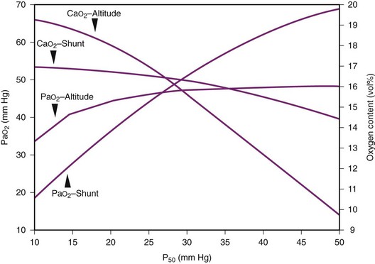
These two situations demonstrate that a leftward shift of the oxyhemoglobin dissociation curve significantly improves arterial oxygen content in the case of high-altitude hypoxemia but not in the case of a large shunt. This observation is consistent with the general finding of a right-shifted curve in patients, such as those with cyanotic heart disease, who have a right-to-left shunt.62 In these cases, a left-shifted curve is not beneficial because only a trivial improvement in Cc′O2 (and thus in PAO2) is obtained. Teleologically, it may be argued that in the presence of hypoxemia, at approximately equal arterial oxygen contents, the body prefers higher oxygen tensions (i.e., right shift), but if arterial oxygen content can be significantly improved, despite a decrease in oxygen tension, a left shift is preferred.
H Example 4: Mathematical/Computer Model for Extracorporeal Membrane Oxygenation
Extracorporeal membrane oxygenation (ECMO) is sometimes used to treat respiratory failure that is refractory to more conservative measures.16 Clinical experience with ECMO is limited, and even clinicians familiar with the therapy may disagree about its potential benefits in a particular clinical setting. This is especially true if the patient has a high CO (e.g., 20 L/min) and the ECMO pump is limited to much smaller flows (e.g., 5 L/min). In the example that follows, we describe how a computer model may be designed to facilitate management decisions for patients being considered for venovenous ECMO.
A mathematical model of the venovenous ECMO situation may be developed on the basis of the shunt equation,56 the Hill model for the oxyhemoglobin dissociation curve,57 Doyle’s equation for arterial oxygen tension as a function of cardiorespiratory parameters,58 and the schematic diagram for venovenous ECMO shown in Figure 4-15. The relevant equations are given in Figure 4-16. The model may be solved for various hypothetical clinical circumstances using an equation solver package. In this instance, we used EUREKA (Borland International, Scotts Valley, CA), a DOS-based commercial computer software package for solving systems of equations.
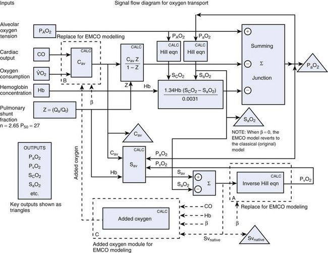
 , oxygen consumption; Svnative, mixed venous oxygen saturation in the absence of ECMO support.
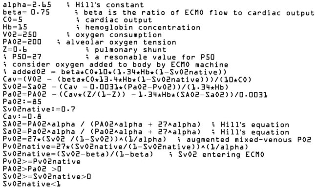
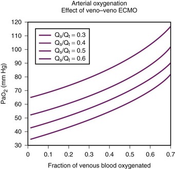
Some sample results are shown in Figure 4-17. The patient’s parameters were as follows: CO = 5 L/min;  = 250 mL/min; Hb = 15 g/dL; Qs/Qt = 0.5; PAO2 = 200 mm Hg. The oxygenator oxygen tension output was sufficient to result in complete hemoglobin saturation.
I Discussion
1. It relies on well-established physiologic relationships (e.g., alveolar gas equation, pulmonary shunt equation).
2. It permits insight into physiologic issues not generally attainable in other ways.
4. It potentially reduces the need to carry out animal experimentation.
Three drawbacks to the method exist:
1. It is no better than the equations on which it is based.
2. It may not be convincing to some physiologists who would be satisfied only by confirmatory experimental results.
One potential difficulty with such modeling methods is that the results obtained depend critically on the equations used. If the equations are known from first principles (e.g., alveolar gas equation, pulmonary shunt equation), this is not an issue, but with empirical formulas, alternative equations may possibly produce different results. An example is the equation for the oxyhemoglobin dissociation curve, which has many competing formulations.61–64 In that example, we used the formulation given by Hill.64
J Utility
On the basis of a model constructed for the time point when the data were gathered, one could explore, for example, the effect of augmenting CO and mixed venous oxygen tension in the ECMO situation. Without a model to describe this problem, the best that can be done is to fit empirical curves to experimental data. However, with a model, one can easily ask “what if” questions, such as, What happens when the ratio of pump oxygenator flow to CO is set at a particular value?.80
A good example is a question frequently asked in respiratory physiology: How does a patient’s alveolar-arterial oxygen tension difference change with reduced inspired oxygen tension? The first attempt at answering this question used pulse oximetry to infer arterial oxygen tension in volunteers subjected to controlled hypoxia by rebreathing.81 A subsequent study took a more direct approach by cannulating the radial artery of elderly respiratory patient volunteers and drawing off serial arterial blood samples as the patients were subjected to hypoxemia in a hypobaric chamber.83 Both of these studies were performed in 1974. The latter investigation was sufficiently invasive (and possibly risky) that many hospital ethics committees would not have approved it under current guidelines.
VIII Selected Dimensional Equivalents
Discussions regarding physics in anesthesia may be confusing because of the variety of units used in the clinical literature. The list in Box 4-1 is a compilation of units and equivalents that one is likely to encounter.
X Clinical Pearls
• An important formula that quantifies the relationship of pressure, flow, and resistance in laminar flow systems is given by the Hagen-Poiseuille equation. This law states that the fluid flow rate through a horizontal straight tube of uniform bore is proportional to the pressure gradient and the fourth power of the radius and is related inversely to the viscosity of the gas and the length of the tube. This law is valid for laminar flow conditions only.
• When the flow rate exceeds a critical velocity (the flow velocity below which flow is laminar), the flow loses its laminar parabolic velocity profile, becomes disorderly, and is termed turbulent. If turbulent flow exists, the relationship between pressure drop and flow is no longer governed by the Hagen-Poiseuille equation. Instead, the pressure gradient required (or the resistance encountered) during turbulent flow varies as the square of the gas flow rate. In addition, flow becomes inversely related to gas density rather than viscosity (as occurs with laminar flow).
• Clinically, airway-obstructing conditions such as epiglottitis or inhaled foreign bodies are often best modeled as breathing through an orifice. Under such conditions, the approximate flow across the orifice varies inversely with the square root of the gas density, in contrast to laminar flow conditions, in which gas flow varies inversely with gas viscosity. In such conditions, the low density of helium allows it to play a significant clinical role in the management of some forms of airway obstruction.
• Laplace’s law predicts that for two alveoli of unequal size but equal surface tension, the smaller alveolus experiences a larger intra-alveolar pressure than the larger alveolus, causing the smaller alveolus to collapse. In real life, however, collapse of the smaller alveolus is prevented through the action of pulmonary surfactant, which serves to decrease alveolar surface tension in the smaller alveolus, resulting in equal pressure in both alveoli.
• One of the most important gas laws in physiology is the ideal (or perfect) gas law, PV = nRT (where P = pressure of gas, V = volume of gas, n = number of moles of the gas in volume V, R = gas constant, and T = absolute temperature). This is the equation for ideal gases, which experience no forces of interaction. Real gases, however, experience intermolecular attraction (van der Waals forces), which requires that the pressure-volume gas law be written in a more complex form.
• Most flowmeters measure the drop in pressure that occurs when a gas passes through a known resistance and correlate this pressure drop to flow. When the resistance is an orifice, resistance depends primarily on gas density. Usually, a given flowmeter is calibrated for a particular gas, such as oxygen or air, with conversion tables available to provide flow data for other gases.
• Fick’s law of diffusion, applicable to gas flow across lung and placental membranes, states that the rate of diffusion of a gas across a barrier is proportional to the concentration gradient for the gas and inversely proportional to the diffusion distance over which the gas molecules must travel.
• There are five main types of oxygen analyzers: paramagnetic analyzers, fuel cell analyzers, oxygen electrodes, mass spectrometers, and Raman spectrographs. All respond to oxygen partial pressure and not to oxygen concentration.
• The concept of minimum alveolar concentration (MAC) does not apply at higher altitudes and should be replaced by the concept of minimal alveolar partial pressure (MAPP).
• The pulmonary shunt equation is used as a foundation upon which arterial oxygenation and gas exchange indices can be studied. Calculation of pulmonary shunt requires the following information: (1) pulmonary end-capillary oxygen content, (2) arterial oxygen content, and (3) mixed venous oxygen content.
All references can be found online at expertconsult.com.
11 Sherwood L. Human physiology: From cells to systems, ed 2. St. Paul, MN: West Publishing; 1993.
20 Kemper KJ, Ritz RH, Benson MS, Bishop MS. Helium-oxygen mixture in the treatment of postextubation stridor in pediatric trauma patients. Crit Care Med. 1991;19:356–359.
23 Rodrigo GJ, Rodrigo C, Pollack CV, Rowe B. Use of helium-oxygen mixtures in the treatment of acute asthma: A systematic review. Chest. 2003;123:891–896.
25 Khanlou H, Eiger G. Safety and efficacy of heliox as a treatment for upper airway obstruction due to radiation-induced laryngeal dysfunction. Heart Lung. 2001;30:146–147.
26 Polaner DM. The use of heliox and the laryngeal mask airway in a child with an anterior mediastinal mass. Anesth Analg. 1996;82:208–210.
42 Straus C, Louis B, Isabey D, et al. Contribution of the endotracheal tube and the upper airway to breathing workload. Am J Respir Crit Care Med. 1998;157:23–30.
49 Bolder PM, Healy TE, Bolder AR, et al. The extra work of breathing through adult endotracheal tubes. Anesth Analg. 1986;65:853–859.
50 Davis PD, Kenny GNC. Basic physics and measurement in anaesthesia, ed 5. Philadelphia: Elsevier Health Science; 2003.
54 James MF, White JF. Anesthetic considerations at moderate altitude. Anesth Analg. 1984;63:1097–1105.
78 Herrick IA, Champion LK, Froese AB. A clinical comparison of indices of pulmonary gas exchange with changes in the inspired oxygen concentration. Can J Anaesth. 1990;37:69–76.
1 Zumdahl SS, Zumdahl SA. Chemistry, ed 8. Belmont, CA: Brooks Cole; 2008.
2 Moran MJ, Shapiro HN. Fundamentals of engineering thermodynamics, ed 6. Hoboken, NJ: Wiley; 2007.
3 Boltz RE, Tuve GL. CRC Handbook of tables for applied engineering science, ed 2. Cleveland, OH: CRC Press; 1973.
4 Haynes WM. CRC Handbook of chemistry and physics, ed 91. Boca Raton, FL: CRC Press; 2010.
5 Askeland DR, Phule PP. The science and engineering of materials, ed 5. Toronto: Thompson; 2006.
6 Benumof JL, Scheller MS. The importance of transtracheal jet ventilation in the management of the difficult airway. Anesthesiology. 1989;71:769–778.
7 Streeter VL, Wylie EB, Bedford KW. Fluid mechanics, ed 9. New York: McGraw-Hill; 1998.
8 White FM. Fluid mechanics, ed 6. New York: McGraw-Hill; 2007.
9 Zuck D. Osborne Reynolds, 1842-1912, and the flow of fluids through tubes. Br J Anaesth. 1971;43:1175–1182.
10 Wright PE, Marini JJ, Bernard GR. In vitro versus in vivo comparison of endotracheal tube airflow resistance. Am Rev Respir Dis. 1989;140:10–16.
11 Sherwood L. Human physiology: From cells to systems, ed 2. St. Paul, MN: West Publishing; 1993.
12 Delaney WA, Kaiser RE, Jr. Percutaneous transtracheal jet ventilation made easy. Anesthesiology. 1991;74:952.
13 Meyer PD. Emergency transtracheal jet ventilation system. Anesthesiology. 1990;73:787–788.
14 Sprague DH. Transtracheal jet oxygenator from capnographic monitoring components. Anesthesiology. 1990;73:788.
15 Doyle DJ, Zawacki J. Importance of catheter resistance in transtracheal jet ventilation. Can J Anaesth. 1993;40:A37.
16 Zapol WM, Snider MT, Hill JD, et al. Extracorporeal membrane oxygenation in severe acute respiratory failure: A randomized prospective study. JAMA. 1979;242:2193–2196.
17 Hill DW. Physics applied to anaesthesia: VI. Gases and vapours (2). Br J Anaesth. 1966;38:753–759.
18 Rudow M, Hill AB, Thompson NW, Finch JS. Helium-oxygen mixtures in airway obstruction due to thyroid carcinoma. Can Anaesth Soc J. 1986;33:498–501.
19 Duncan PG. Efficacy of helium-oxygen mixtures in the management of severe viral and post-intubation croup. Can Anaesth Soc J. 1979;26:206–212.
20 Kemper KJ, Ritz RH, Benson MS, Bishop MS. Helium-oxygen mixture in the treatment of postextubation stridor in pediatric trauma patients. Crit Care Med. 1991;19:356–359.
21 Lu TS, Ohmura A, Wong KC, Hodges MR. Helium-oxygen in treatment of upper airway obstruction. Anesthesiology. 1976;45:678–680.
22 Skrinskas GJ, Hyland RH, Hutcheon MA. Using helium-oxygen mixtures in the management of acute upper airway obstruction. Can Med Assoc J. 1983;128:555–558.
23 Rodrigo GJ, Rodrigo C, Pollack CV, Rowe B. Use of helium-oxygen mixtures in the treatment of acute asthma: A systematic review. Chest. 2003;123:891–896.
24 Ho AM, Lee A, Karmakar MK, et al. Heliox vs air-oxygen mixtures for the treatment of patients with acute asthma: A systematic overview. Chest. 2003;123:882–890.
25 Khanlou H, Eiger G. Safety and efficacy of heliox as a treatment for upper airway obstruction due to radiation-induced laryngeal dysfunction. Heart Lung. 2001;30:146–147.
26 Polaner DM. The use of heliox and the laryngeal mask airway in a child with an anterior mediastinal mass. Anesth Analg. 1996;82:208–210.
27 Gottfried SP, Emili JM. Noninvasive monitoring of respiratory mechanics. In: Nochomovitz ML, Cherniac NS. Noninvasive respiratory monitoring. New York: Churchill Livingstone, 1986.
28 Ferris BG, Jr., Mead J, Opie LH. Partitioning of respiratory flow resistance in man. J Appl Physiol. 1964;19:653–658.
29 Boretos JW, Battig CG, Goodman L. Decreased resistance to breathing through a polyurethane pediatric endotracheal tube. Anesth Analg. 1972;51:292–296.
30 Weissman C, Askanazi J, Rosenbaum SH, et al. Response to tubular airway resistance in normal subjects and postoperative patients. Anesthesiology. 1986;64:353–358.
31 Wall MA. Infant endotracheal tube resistance: Effects of changing length, diameter, and gas density. Crit Care Med. 1980;8:38–40.
32 Gal TJ. Pulmonary mechanics in normal subjects following endotracheal intubation. Anesthesiology. 1980;52:27–35.
33 Nadel JA. Mechanisms controlling airway size. Arch Environ Health. 1963;7:179–182.
34 Hegyi T, Hiatt IM. Respiratory index: A simple evaluation of severity of idiopathic respiratory distress syndrome. Crit Care Med. 1979;7:500–501.
35 Aalto-Setälä M, Heinonen J. Resistance to gas-flow of endobronchial tubes. Ann Chir Gynaecol Fenn. 1973;62:271–276.
36 Holst M, Striem J, Hedenstierna G. Errors in tracheal pressure recording in patients with a tracheostomy tube: A model study. Intensive Care Med. 1990;16:384–389.
37 Michels A, Landser FJ, Cauberghs M, Van de Woestijne KP. Measurement of total respiratory impedance via the endotracheal tube: A model study. Bull Eur Physiopathol Respir. 1986;22:615–620.
38 Gaensler EA, Maloney JV, Jr., Bjork VO. Bronchospirometry: II. Experimental observations and theoretical considerations of resistance breathing. J Lab Clin Med. 1952;39:935–953.
39 Gal TJ, Suratt PM. Resistance to breathing in healthy subjects following endotracheal intubation under topical anesthesia. Anesth Analg. 1980;59:270–274.
40 Hicks GH. Monitoring respiratory mechanics. Probl Respir Care. 1989;2:191.
41 Manczur T, Greenough A, Nicholson GP, Rafferty GF. Resistance of pediatric and neonatal endotracheal tubes: Influence of flow rate, size, and shape. Crit Care Med. 2000;28:1595–1598.
42 Straus C, Louis B, Isabey D, et al. Contribution of the endotracheal tube and the upper airway to breathing workload. Am J Respir Crit Care Med. 1998;157:23–30.
43 Beatty PC, Healy TE. The additional work of breathing through Portex Polar “Blue-Line” pre-formed paediatric tracheal tubes. Eur J Anaesthesiol. 1992;9:77–83.
44 Fawcett W, Ooi R, Riley B. The work of breathing through large-bore intravascular catheters. Anesthesiology. 1992;76:323–324.
45 Mullins JB, Templer JW, Kong J, et al. Airway resistance and work of breathing in tracheostomy tubes. Laryngoscope. 1993;103:1367–1372.
46 Ooi R, Fawcett WJ, Soni N, Riley B. Extra inspiratory work of breathing imposed by cricothyrotomy devices. Br J Anaesth. 1993;70:17–21.
47 Petros AJ, Lamond CT, Bennett D. The Bicore pulmonary monitor: A device to assess the work of breathing while weaning from mechanical ventilation. Anaesthesia. 1993;48:985–988.
48 Shikora SA, Bistrian BR, Borlase BC, et al. Work of breathing: Reliable predictor of weaning and extubation. Crit Care Med. 1990;18:157–162.
49 Bolder PM, Healy TE, Bolder AR, et al. The extra work of breathing through adult endotracheal tubes. Anesth Analg. 1986;65:853–859.
50 Davis PD, Kenny GNC. Basic physics and measurement in anaesthesia, ed 5. Philadelphia: Elsevier Health Science; 2003.
51 Zin WA, Pengelly LD, Milic-Emili J. Single-breath method for measurement of respiratory mechanics in anesthetized animals. J Appl Physiol. 1982;52:1266–1271.
52 West JB. Respiratory physiology. The essentials, ed 8. Philadelphia: Lippincott Williams & Wilkins; 2008.
53 Chathurn R, Miresles-Cabodevila E. Handbook of respiratory care, ed 3. Sudbury, MA: Jones & Bartlett; 2010.
54 James MF, White JF. Anesthetic considerations at moderate altitude. Anesth Analg. 1984;63:1097–1105.
55 Doyle DJ. Arterial/alveolar oxygen tension ratio: A critical appraisal. Can Anaesth Soc J. 1986;33:471–474.
56 Viale JP, Percival CJ, Annat G, et al. Arterial-alveolar oxygen partial pressure ratio: A theoretical reappraisal. Crit Care Med. 1986;14:153–154.
57 Torda TA. Alveolar-arterial oxygen tension difference: A critical look. Anaesth Intensive Care. 1981;9:326–330.
58 Kelman GR, Nunn JF, Prys-Roberts C, Greenbaum R. The influence of cardiac output on arterial oxygenation: A theoretical study. Br J Anaesth. 1967;39:450–458.
59 Standardization of definitions and symbols in respiratory physiology. Fed Proc. 1950;9:602–605.
60 Jones N. Blood gases and acid-base physiology, ed 2. New York: Thieme-Stratton; 1987.
61 Aberman A, Cavanilles JM, Trotter J, et al. An equation for the oxygen hemoglobin dissociation curve. J Appl Physiol. 1973;35:570–571.
62 Kelman GR. Digital computer subroutine for the conversion of oxygen tension into saturation. J Appl Physiol. 1966;21:1375–1376.
63 Lobdell DD. An invertible simple equation for computation of blood O2 dissociation relations. J Appl Physiol. 1981;50:971–973.
64 Schneider AJ, Stockman JA, 3rd., Oski FA. Transfusion nomogram: An application of physiology to clinical decisions regarding the use of blood. Crit Care Med. 1981;9:469–473.
65 Severinghaus JW. Simple, accurate equations for human blood O2 dissociation computations. J Appl Physiol. 1979;46:599–602.
66 Rasanen J, Downs JB, Malec DJ, Oates K. Oxygen tensions and oxyhemoglobin saturations in the assessment of pulmonary gas exchange. Crit Care Med. 1987;15:1058–1061.
67 Rodgers E. TK Solver: A new concept in problem solving software. PC World. 1983;1:93.
68 Konopasek M, Jayaraman S. Constant and declarative languages for engineering applications: The TK Solver contribution. Proc IEEE. 1985;73:1791.
69 Konopasek M, Jayaraman S. The TK Solver book: A guide to problem-solving in science, engineering, business and education. Berkeley, CA: Osborne/McGraw-Hill; 1984.
70 Kanber GJ, King FW, Eshchar YR, Sharp JT. The alveolar-arterial oxygen gradient in young and elderly men during air and oxygen breathing. Am Rev Respir Dis. 1968;97:376–381.
71 Farhi LE, Rahn H. A theoretical analysis of the alveolar-arterial O2 difference with special reference to the distribution effect. J Appl Physiol. 1955;7:699–703.
72 Gilbert R, Auchincloss JH, Jr., Kuppinger M, Thomas MV. Stability of the arterial/alveolar oxygen partial pressure ratio: Effects of low ventilation/perfusion regions. Crit Care Med. 1979;7:267–272.
73 Gilbert R, Keighley JF. The arterial-alveolar oxygen tension ratio: An index of gas exchange applicable to varying inspired oxygen concentrations. Am Rev Respir Dis. 1974;109:142–145.
74 Shapiro AR, Virgilio RW, Peters RM. Interpretation of alveolar-arterial oxygen tension difference. Surg Gynecol Obstet. 1977;144:547–552.
75 Peris LV, Boix JH, Salom JV, et al. Clinical use of the arterial/alveolar oxygen tension ratio. Crit Care Med. 1983;11:888–891.
76 Goldfarb MA, Ciurej TF, McAslan TC, et al. Tracking respiratory therapy in the trauma patient. Am J Surg. 1975;129:255–258.
77 Covelli HD, Nessan VJ, Tuttle WK, 3rd. Oxygen derived variables in acute respiratory failure. Crit Care Med. 1983;11:646–649.
78 Herrick IA, Champion LK, Froese AB. A clinical comparison of indices of pulmonary gas exchange with changes in the inspired oxygen concentration. Can J Anaesth. 1990;37:69–76.
79 Zetterstrom H. Assessment of the efficiency of pulmonary oxygenation: The choice of oxygenation index. Acta Anaesthesiol Scand. 1988;32:579–584.
80 Torrance J, Jacobs P, Restrepo A, et al. Intraerythrocytic adaptation to anemia. N Engl J Med. 1970;283:165–169.
81 Eaton JW, Skelton TD, Berger E. Survival at extreme altitude: Protective effect of increased hemoglobin-oxygen affinity. Science. 1974;183:743–744.
82 Hebbel RP, Eaton JW, Kronenberg RS, et al. Human llamas: Adaptation to altitude in subjects with high hemoglobin oxygen affinity. J Clin Invest. 1978;62:593–600.
83 Monge C, Whittembury J. Increased hemoglobin-oxygen affinity at extremely high altitudes [Letter]. Science. 1974;186:843.
84 Morpurgo G, Arese P, Bosia A, et al. Sherpas living permanently at high altitutde: A new pattern of adaptation. Proc Natl Acad Sci U S A. 1976;73:747–751.