CHAPTER 11 Neurosurgical Epidemiology and Outcomes Assessment
Concepts—Sources of Error in Analysis
Bias
Structural error, or bias, in contrast, is error that tends to apply specifically to one group of subjects in a study and is a consequence of intentional or unintentional features of the study design itself. This is error designed into the experiment and is not measurable or controllable by statistical techniques, but it can be minimized with proper experimental design. For example, if we are determining the normal head size of term infants by measuring the head size of all such patients born over a 1-week period, we have a high probability of introducing random error into our reported rate because we are considering a small sample. We can measure this tendency of random error in the form of a confidence interval around the reported head size. The larger the confidence interval, the higher the chance that our reported head size differs from the true average head size of our population of interest. We can solve this problem by increasing the sample size without any other change in experimental technique. Conversely, if we choose to conduct our study only in the newborn intensive care unit, with exclusion of the well-child nursery, and reported our measurements as pertaining to newborn children in general, we have introduced a structural error, or bias, into our experimental design. No statistical test that we can apply to our data set will alert us that this is occurring, nor will measures such as increasing the number of patients in our study help solve the problem. In considering the common study designs enumerated later, note how different types of studies are subject to different biases and how the differences in study design arise out of an attempt to control for bias.1
Control of Confounding Variables
Noise—Statistical Analysis in Outcomes Assessment
Alpha and Beta Error and Power
The second, more common error is a type II or β error.2 This represents the probability of incorrectly concluding that a difference does not exist between therapies when in fact it does. This is analogous to missing the signal for the noise. Here, the key issue is the natural degree of variability among study subjects, independent of what might be due to treatment effects. When small but real differences exist between groups and there is enough variability among subjects, the study requires a large sample size to be able to show a difference. Missing the difference is a β error, and the power of a study is 1 − β. Study power is driven by sample size. The larger the sample, the greater the power to resolve small differences between groups.
Frequently, when a study fails to show a difference between groups, there is a tendency to assume that there is in fact no difference between them.3 What is needed is an assessment of the likelihood of a difference being detected, given the sample size and subject variability. Although the authors should provide this, they frequently do not, thereby leaving readers to perform their own calculations or refer to published nomograms.4,5 Arbitrarily, we say that a power of 80%, or the chance of detecting a difference of a specified amount given a sample size of n, is acceptable. If the penalties for missing a difference are high, other values for power can be selected, but the larger the power desired, the larger the sample size required.
Statistics and Probability in Diagnosis
Pretest and Posttest Probability—A Bayesian Approach
At the onset, certain quickly ascertainable features about a clinical encounter should lead to the formation of a baseline probability of the most likely diagnoses for the particular clinical findings. In the example just presented, among all children seen by a neurosurgeon within 3 months of initial shunt placement, about 30% will subsequently be found to have shunt malfunction.6 Before any tests are performed or even a physical examination completed, elements of the history provided allow the clinician to form this first estimate of the likelihood of shunt failure. The remainder of the history and physical findings allow revision of that probability, up or down. This bayesian approach to diagnosis requires some knowledge of how particular symptoms and signs affect the baseline, or the “pretest” probability of an event. The extent to which a particular clinical finding or diagnostic study influences the probability of a particular end diagnosis is a function of its sensitivity and specificity, which may be combined into the clinically more useful likelihood ratio.7 Estimates of the pretest probability of disease tend to be situation specific; for example, the risk of failure of a cerebrospinal fluid (CSF) shunt after placement is heavily dependent on the age of the patient and the time elapsed since the last shunt-related surgical procedure.8 Individual practitioners can best provide their own data for this by studying their own practice patterns.
Properties of Diagnostic Tests
Elements of the history, physical examination, and subsequent diagnostic studies can all be assessed to describe their properties as predictors of an outcome of interest. These properties may be summarized as sensitivity, specificity, positive and negative predictive values, and likelihood ratios, as illustrated in Table 11-1.
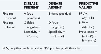
Sensitivity indicates the percentage of patients with a given illness who have a positive clinical finding or study. In other words, that a straight leg raise test has a sensitivity of 80% for lumbar disk herniation in the setting of sciatic pain means that 80 of 100 patients with sciatica and disk herniation do, in fact, have a positive straight leg raise test.9 In Table 11-1, sensitivity is equal to a/(a + c). Conversely, specificity, equal to d/(b + d) in Table 11-1, refers to the number of patients without a clinical diagnosis who also do not have a clinical finding. Again, using the example of the evaluation of low back pain in patients with sciatica, a positive straight leg raise test has about 40% specificity, which means that of 100 patients with sciatica but without disk herniation, 40 will have a negative straight leg raise test.
Sensitivity and specificity are difficult to use clinically because they describe clinical behavior in a group of patients known to carry the diagnosis of interest. These properties provide no information about performance of the clinical factor in patients who do not have the disease and who probably represent the majority of patients seen. Sensitivity ignores the important category of false-positive results (Table 11-1, B), whereas specificity ignores false-negative results (Table 11-1, C). If the sensitivity of a finding is very high (e.g., >95%) and the disease is not overly common, it is safe to assume that there will be few false-negative results (C in Table 11-1 will be small). Thus, the absence of a finding with high sensitivity for a given condition will tend to rule out the condition. When the specificity is high, the number of false-positive results is low (B in Table 11-1 will be small), and the absence of a symptom will tend to rule in the condition. Epidemiologic texts have suggested the mnemonics SnNout (when sensitivity is high, a negative or absent clinical finding rules out the target disorder) and SpPin (when specificity is very high, a positive study rules in the disorder), although some caution may be in order when applying these mnemonics strictly.10
A key component of these latter two values is the underlying prevalence of the disease. Examine Table 11-2. In both the common disease and rare disease case, the sensitivity and specificity for the presence or absence of a particular sign are each 90%, but in the common disease case, the total number of patients with the diagnosis is much larger, thereby leading to much higher positive and lower negative predictive values. When the prevalence of the disease drops, the important change is the relative increase in the number of false versus true positives, with the reverse being true for false versus true negatives.
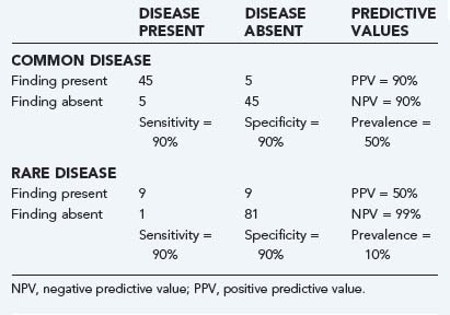
The impact of prevalence plays a particularly important role when one tries to assess the role of screening studies in which there is only limited clinical evidence that a disease process is present. Examples include the use of screening magnetic resonance imaging studies for cerebrovascular aneurysms in patients with polycystic kidney disease11 and routine use of CT for follow-up after shunt insertion12 and for determining cervical spine instability in patients with Down syndrome,13 as well as to search for cervical spine injuries in polytrauma patients.14,15 In these situations, the low prevalence of the disease makes false-positive results likely, particularly if the specificity of the test is not extremely high, and usually results in additional, potentially more hazardous and expensive testing.
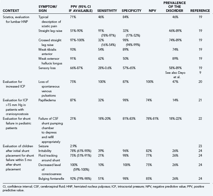
Likelihood ratios (LRs) are an extension of the previously noted properties of diagnostic information. LRs express the odds (rather than the percentage) of a patient with a target disorder having a particular finding present as compared with the odds of the finding in patients without the target disorder. An LR of 4 for a clinical finding indicates that it is four times as likely for a patient with the disease to have the finding as those without the disease. The advantage of this approach is that odds ratios, which are based on sensitivity and specificity, do not have to be recalculated for any given prevalence of a disease. In addition, if one starts with the pretest odds of a disease, this may be simply multiplied by the LR to generate the posttest odds of a disease. Nomograms exist to further simplify this process.16 A number of useful articles and texts are available to the reader for further explanation.17,18 Table 11-3 gives examples of the predictive values of selected symptoms and signs encountered in clinical neurosurgical conditions.9,19–24
Clinical Decision Rules
The preceding examples demonstrate the mathematical consequences of the presence of a single symptom or sign on the diagnostic process. The usual diagnostic process involves the integration of different symptoms and signs, often simultaneous with the process of generating a differential diagnosis. Clinical decision rules or decision instruments allow integration of multiple symptoms or signs into a diagnostic algorithm. The desired properties of such algorithms depend on the disease process studied, the consequences of false-positive and false-negative results, and the risk and cost of evaluation maneuvers. For example, the National Emergency X-Radiography Utilization Study (NEXUS) sought to develop a clinical prediction rule to determine which patients require cervical spine x-ray assessment after blunt trauma.15
Measurement in Clinical Neurosurgery
Techniques of Measurement
Quantifying clinical findings and outcomes remains one of the largest stumbling blocks in performing and interpreting clinical research. Although outcomes such as mortality and some physical attributes such as height and weight are easily assessed, many of the clinical observations and judgments that we make are much more difficult to measure. All measurement scales should be valid, reliable, and responsive. A scale is valid if it truly measures what it purports to measure. It is reliable when it reports the same result for the same condition, regardless of who applies it or when they do so. It is responsive when meaningful changes in the item or event being measured are reflected as changes in the scale.25 The complexity of neurologic assessment has led to a proliferation of such measurement scales.26
Validity
Content validity is a similar concept that arises out of scale development. In the course of developing scales, a series of domains are determined. For example, again referring to the activities of daily living, the functional independence measure has domains of self-care, sphincter control, mobility and transfer, location, communication, and social cognition.27 The more completely that a scale addresses the perceived domains of interest, the better its content validity.
Criterion validity refers to performance of the new scale in comparison to a previously established standard. Simplified shorter scales that are more readily usable in routine clinical practice should be expected to have criterion validity when compared with longer, more complex research-oriented scales.28
Reliability
To be clinically useful, a scale should give a consistent report when applied repeatedly to a given patient. Reliability and discrimination are intimately linked in that the smaller the error attributable to measurement, the finer the resolving power of the measurement instrument. Measurement in part involves determining differences, so the discriminatory power of an instrument is of critical importance. Although often taught otherwise, reliability and agreement are not the same thing. An instrument that produces a high degree of agreement and no discrimination between subjects is, by definition, unreliable. This need for reproducibility and discrimination is dependent not only on the nature of the measurement instrument but also on the nature of the system being measured. An instrument found reliable in one setting may not be so in another if the system being measured has changed dramatically. Mathematically, reliability is equal to subject variability divided by the sum of subject and measurement variability.25 Thus, the larger the variability (error) caused by measurement alone, the lower the reliability of a system. Similarly, for a given measurement error, the larger the degree of subject variability, the less the impact of measurement error on overall reliability. Reliability testing involves repeated assessments of subjects by the same observers, as well as by different observers.
Reliability is typically measured by correlation coefficients, with values ranging between 0 and 1. Although there are several different statistical methods of determining the value of the coefficient, a common strategy involves the use of analysis of variance (ANOVA) to produce an intraclass correlation coefficient (ICC).29 The ICC may be interpreted as representing the percentage of total variability attributable to subject variability, with 1 being perfect reliability and 0 being no reliability. Reliability data reported as an ICC can be converted into a range of scores expected simply because of measurement error. The square root of (1 − ICC) gives the percentage of the standard deviation of a sample expected to be associated with measurement error. A quick calculation brings the ICC into perspective. For an ICC of 0.9, the error associated with measurement is (1 − 0.9)0.5, or about 30% of the standard deviation.25 Reliability measures can also be reported with the κ statistic, discussed more fully in the next section as a measure of clinical agreement.30
Internal consistency is a related property of scales that are used for measurement. Because scales should measure related aspects of a single dimension or construct, responses on one question should have some correlation to responses on another question. Although a high degree of correlation renders a question redundant, very limited correlation raises the possibility that the question is measuring a different dimension or construct. This has the effect of adding additional random variability to the measure. There are a variety of statistics that calculate this parameter, the best known of which is Cronbach’s alpha coefficient.31 Values between 0.7 and 0.9 are considered acceptable.25
Clinical Agreement
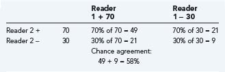
One of the common statistical ways to measure agreement is the κ statistic.32,33 It attempts to compensate for the likelihood of chance agreement when only a few possible choices are available. If two observers identify the presence of a clinical finding 70% of the time in a particular patient population, by chance they will agree on the finding 58% of the time (Table 11-4). If they actually agree 80% of the time, the κ statistic for this clinical parameter is 80% to 58% actual agreement beyond chance and 100% to 58% potential agreement beyond chance. This is equal to 0.52. Interpretation of these κ values is somewhat arbitrary, but by convention, κ values of 0 to 0.2 indicate slight agreement; 0.2 to 0.4, fair agreement; 0.4 to 0.6, moderate agreement; and 0.8 to 1.0, high agreement.34
The concept of clinical agreement can be broadened to apply not only to individual symptoms, signs, or tests but also to whole diagnoses; for example, Kestle and colleagues reported that a series of objective criteria for establishing the diagnosis of shunt malfunction have a high degree of clinical agreement (κ = 0.81) with the surgeon’s decision to revise the shunt.35
The κ statistic is commonly used to report the agreement beyond that expected by chance alone and is easy to calculate. However, concern has been raised about its mathematical rigor and its usefulness for comparison across studies (for a detailed discussion see http://ourworld.compuserve.com/homepages/jsuebersax/kappa.htm#start).36,37
Responsiveness
Measurement is largely a matter of discrimination among different states of being, but change needs to be both detected and meaningful. Between 1976 and 1996, Bracken and associates performed a series of randomized controlled trials (RCTs) to evaluate the role of corticosteroids in the management of acute spinal cord injury.38–40 In the last two trials, the main outcome measure was performance on the American Spinal Cord Injury Association (ASIA) scale. Both studies demonstrated small positive benefits in preplanned subgroup analyses for patients receiving methylprednisolone. Subsequent to their publication, however, controversy arose regarding whether the degree of change demonstrated on the ASIA scale is clinically meaningful and justifies the perceived risk of increased infection rates with the therapy. The scale itself assesses motor function in 10 muscle groups on a 6-point scale from 0 (no function) to 5 (normal function and resistance). Sensory function is assessed in 28 dermatomes for both pinprick and light touch. In the first National Acute Spinal Cord Injury Study (NASCIS 1), the net benefit of methylprednisolone was a mean motor improvement of 6.7 versus 4.8 on a scale of 0 to 70. What is unclear from the scale is whether changes of this degree produce any significant functional improvement in a spinal cord injury patient.41–43 Presumably seeking to address this question, the last of these trials included a separate functional assessment, the functional independence measure. This multidimensional instrument assesses the need for assistance in a variety of activities of daily living. A change in this measure, at least on face, produces a more obvious change in functional state than does the ASIA scale. Indeed, a small improvement in the sphincter control subgroup of the scale was seen in the NASCIS 3 trial, although considering the scale as a whole, no improvement was seen.38
Measurement Instruments
A large number of measurement instruments are now in regular use for the assessment of neurosurgical outcomes. Table 11-5 lists just a few of these,44–84 as do other summaries.85 Several types of instruments are noted. First, a number of measures focus on physical findings, such as the Glasgow Coma Scale (GCS), Mini-Mental Status Examination, and House-Brackmann score for facial nerve function. These measures are specific to a disease process or body system. A second group of instruments focus on the functional limitations produced by the particular system insult. A third group of instruments look at the role that functional limitations play in the general perception of health. Instruments that assess health status or health perceptions, such as the 36-item short-form health survey (SF-36) or Sickness Impact Profile, measure in multiple domains and are thought of as generic instruments applicable to a wide variety of illnesses. Others instruments include both general and disease-specific questions. The World Health Organization defines health as “a state of complete physical, mental, and social well-being and not merely the absence of disease or infirmity.”86 In this context, it is easy to see the importance of broader measures of outcome that assess quality of life. Finally, economic measures such as health utilities indices are designed to translate health outcomes into monetary terms.87
| DISEASE PROCESS/SCALE | FEATURES | REFERENCE |
|---|---|---|
| Head Injury | ||
| Glasgow Coma Scale (GCS) | Examination scale: Based on eye (1-4 points), verbal (1-5 points), and motor assessment (1-6 points) | 44 |
| Glasgow Outcome Scale | 1, Dead; 2, vegetative; 3, severely disabled; 4, moderately disabled; 5, good | 45 |
| DRS (disability rating scale) | Score of 0 (normal) to 30 (dead); incorporates elements of the GCS and functional outcome | 46 |
| Ranchos Los Amigos | I, No response; II, generalized response to pain; III, localizes; IV, confused/agitated; V, confused/nonagitated; VI, confused/appropriate; VII, automatic/appropriate; VII, purposeful/appropriate | 47 |
| Mental Status Testing | ||
| Folstein’s Mini-Mental State Examination | 11 Questions: orientation, registration (repetition), attention (serial 7s), recall, language (naming, multistage commands, writing, copying design) | 48, 49 |
| Cognitive Testing | ||
| Wechsler Adult Intelligence Scale (WAIS) | The standard IQ test for adults with verbal (information, comprehension, arithmetic, similarities, digit span, vocabulary) and performance domains (digit symbols, picture completion, block designs, picture arrangement, object assembly)50 | 51 |
| Epilepsy | ||
| Engel class | ||
Original version had no grade 0 and grade 1 equivalent to grade 2 above
ADLs, activities of daily living; ASIA, American Spinal Cord Injury Association; EORTC, European Organization for Research and Treatment of Cancer; NIH, National Institutes of Health; SF-36, short-form health survey (36 items); WFNS, World Federation of Neurological Surgeons.
Choosing a Specific Measure
Functional outcome measures assess the impact of physiologic changes on more general function. Evidence from these sources may be more compelling than changes in physiologic parameters (see discussion on the NACSIS trials earlier). Even more broadly, health status measures place the loss of function in the context of the patient’s global health picture. These measures are particularly useful when comparing across disease processes or comparing healthy and diseased populations. A common strategy is to incorporate both system/disease-specific and generic outcome measures in the same study. Authors and readers must be clear which of these represents the primary outcome measure of the study. When the purpose of the study is to measure the economic impact of a therapy or its “utility” in an economic context, summary measures that report a single score rather than a series of scores for different domains are necessary. In many cases it is appropriate to have the quality-of-life measure as the principal outcome assessment tool. For example, in assessments of therapy for glioblastoma multiforme, efforts to extend survival have thus far been only minimally successful. Studies focusing on maximizing quality of life with the available modalities are often the best ones to provide information on therapeutic decision making.88
Rating scales and quality-of-life assessment measures need not be limited to research studies. Familiarity with these measures can lead to their introduction into general clinic practice and thereby give the practitioner a more effective way to communicate with others and assess individual results. The “Guidelines for the Management of Acute Cervical Spine and Spinal Cord Injuries” offers as a guideline that the functional independence measure be used as a clinical assessment tool by practitioners when assessing patients with spinal cord injury.89 Practical considerations dictate that instruments used in the conduct of routine care be short and feasible to perform. However, ad hoc modification or simplification of instruments to suit individual tastes or needs voids the instruments’ validation and reduces comparability with other applications. Access to many of the outcome measures listed in Table 11-5 is available through the Internet.
Specific Study Designs
Clinical researchers and clinicians using clinical research must be familiar with the various research designs available and commonly used in the medical literature. To better understand the features of study design, it is helpful to consider factors that limit the ability of a study to answer that question. In this context, it is easier to understand the various permutations of clinical research design. Elementary epidemiology textbooks broadly divide study designs into descriptive and analytic studies (Table 11-6).90 The former seek to describe health or illness in populations or individuals but are not suited to describing causal links or establishing treatment efficacy. Comparisons can be made with these study modalities only on an implicit, or population, basis. Thus, a death rate may be compared with a population norm or with death rates in other countries. Analytic or explanatory studies have the specific purpose of direct comparison between assembled groups and are designed to yield answers concerning causation and treatment efficacy. Analytic studies may be observational, as in case-control and cohort studies, or interventional, as in controlled clinical trials. In addition to being directed at different questions, different study designs are more or less robust in managing the various study biases that must be considered as threats to their validity (Table 11-7).1,91
| EXAMPLE | LIMITATIONS (TYPICAL) | |
|---|---|---|
| Descriptive Studies | ||
| Population correlation studies | Rate of disease in population vs. incidence of exposure in population | No link at the individual level, cannot assess or control for other variables. Used for hypothesis generation only |
| Changes in disease rates over time | No control for changes in detection techniques | |
| Individuals | ||
| Case reports and case series | Identification of rare events, report of outcome of particular therapy | No specific control group or effort to control for selection biases |
| Cross-sectional surveys | Prevalence of disease in sample, assessment of coincidence of risk factor and disease at a single point in time at an individual level | “Snapshot” view does not allow assessment of causation, cannot assess incident vs. prevalent cases. Sample determines degree to which findings can be generalized |
| Descriptive cohort studies | Describes outcome over time for specific group of individuals, without comparison of treatments | Cannot determine causation, risk of sample-related biases |
| Analytic Studies | ||
| Observational | ||
| Case control | Disease state is determined first. Identified control group retrospectively compared with cases for presence of particular risk factor | Highly suspect for bias in selection of control group. Generally can study only one or two risk factors |
| Retrospective cohort studies | Population of interest determined first, outcome and exposure determined retrospectively | Uneven search for exposure and outcome between groups. Susceptible to missing data, results dependent on entry criteria for cohort |
| Prospective cohort studies | Exposure status determined in a population of interest, then monitored for outcome | Losses to follow-up over time, expensive, dependent on entry criteria for cohort |
| Interventional | ||
| Dose escalation studies (phase I) | Risk for injury from dose escalation | Comparison is between doses, not vs. placebo. Determines toxicity not efficacy |
| Controlled nonrandom studies | Allocation to different treatment groups by patient/clinician choice | Selection bias in allocation between treatment groups |
| Randomized controlled trials | Random allocation of eligible subjects to treatment groups | Expensive. Experimental design can limit generalizability of results |
| Meta-analysis | Groups randomized trials together to determine average response to treatment | Limited by quality of original studies, difficulty combining different outcome measures. Variability in base study protocols |
After Hennekens C, Buring J. Epidemiology in Medicine. Boston: Little, Brown; 1987.
TABLE 11-7 Common Biases in Clinical Research
| BIAS NAME | EXPLANATION |
|---|---|
| Sampling Biases | |
| Prevalence-incidence | Drawing a sample of patients late in a disease process excludes those who have died of the disease early in its course. Prevalent (existing) cases may not reflect the natural history of incident (newly diagnosed) cases |
| Unmasking | In studies investigating causation, factors that cause symptoms, which in turn cause a more diligent search for the disease of interest. An example might be whether a particular medication caused headaches, which led to the performance of more magnetic resonance imaging studies and resulted in an increase in the diagnosis of arachnoid cysts in patients taking the medication. The conclusion that the medication caused arachnoid cysts would reflect unmasking bias |
| Diagnostic suspicion | A predisposition to consider an exposure as causative prompts a more thorough search for the presence of the outcome of interest |
| Referral filter | Patients referred to tertiary care centers are often not reflective of the population as a whole in terms of disease severity and comorbid conditions. Natural history studies are particularly prone to biases of this sort |
| Chronologic | Patients cared for in previous periods probably underwent different diagnostic studies and treatments. Studies with historical controls are at risk |
| Nonrespondent/volunteer | Patients who choose to respond or not respond to surveys or follow-up assessments differ in tangible ways. Studies with incomplete follow-up or poor response rates are prone to this bias |
| Membership bias | Cases or controls drawn from specific self-selected groups often differ from the general population. The result of this bias is the assumption that the group’s defining characteristic is the cause of their performance with respect to a risk factor |
| Intervention Biases | |
| Co-intervention | Patients in an experimental or control group systematically undergo an additional treatment not intended by the study protocol. If a treatment were significantly more painful than a control procedure, a potential co-intervention would be increased analgesic use postoperatively. A difference in outcome could be due to either the treatment or the co-intervention |
| Contamination | When patients in the control group receive the experimental treatment, the potential differences between the groups are masked |
| Therapeutic personality | In unblinded studies, the belief in a particular therapy may influence the way in which the provider and patient interact and alter the outcome |
| Measurement | |
| Expectation | Prior expectations about the results of an assessment can substitute for actual measurement. In assessments of either diagnosis or therapy, belief in the predictive ability or therapeutic efficacy increases the likelihood that a positive effect will be measured. Unblinded studies and those with a subjective outcome measure are prone to this bias |
| Recall | In cohort and case-control studies, different assessment techniques or frequencies applied to those with the outcome of interest may increase the likelihood of detection of a risk factor, in particular, asking cases multiple times vs. controls improves chances for recall. This bias applies especially to retrospective studies and is the inverse of the diagnostic-suspicion bias (see earlier) |
| Unacceptability | Measurements that are uncomfortable, either physically or mentally, may be avoided by study subjects |
| Unpublished scales | The use of unpublished outcome scales has been shown in certain settings to result in a greater probability of the study finding in favor of experimental treatment91 |
| Analysis | |
| Post hoc significance | When decisions regarding levels of significance or statistical measures to be used are determined after the results are analyzed, it is more likely that a significant result will be found. It is very unlikely that authors would state this in a manuscript, but protection is afforded by publication of the study methods in advance of the study itself |
| Data dredging | Asking multiple questions of a dataset until something with statistical significance is found. Subgroup analysis, depending on whether preplanned and coherent with the study aims and hypotheses, may also fall into this category |
From Sackett DL. Bias in analytic research. J Chronic Dis. 32:51, 1979.
Analytic Studies
Diagnosis and Patient Assessment Studies
Studies looking at the discriminatory power of diagnostic tests or strategies ask the general question, “How well do the results of this diagnostic test predict the presence or absence of the sought-after disease?” Most often such studies take on the general form of a cohort study. The group of patients with the suspected disease is the cohort (e.g., all adult patients undergoing major surgery at a particular institution). The cohort is assessed for the presence of a risk factor (positive duplex scan of the lower extremity for clots) and then monitored for an outcome, which is usually the result of the “gold standard” diagnostic test (presence of deep venous thrombosis on venography).92 Like other cohort studies, studies looking at diagnostic accuracy are susceptible to bias when knowledge of the gold standard result can influence interpretation of the diagnostic study under question, or the reverse. This is similar to recall bias or diagnostic-suspicion bias for the more typical prospective and retrospective cohort studies.
Natural History Studies
Usually a variant of a cohort design, natural history studies observe a group of patients drawn from a defined population over time to determine the occurrence of particular outcome events such as mortality, rebleeding rates, stroke rates, and others. In essence, the study seeks to determine how accurately the future outcome can be predicted by a group of know predictors. Studies of this sort occupy a critical place in clinical reasoning because they can provide information about the consequences of a decision not to treat. Natural history studies do not replace a randomized comparison between placebo and treatment, but they are often the starting point for therapy decisions in the absence of such studies and frequently provide the framework for subsequent randomized comparisons. The line between a natural history study and a case series with long-term follow-up may seem a fine one, but the key is in determining the degree to which the study patients are representative of the population as a whole and the degree to which the follow-up investigations are evenly applied. The literature regarding the debate on the hemorrhage rate for unruptured aneurysms smaller than 1 cm provides numerous examples of this type of study and highlights the potential bias in studies of this type.93–96 Critical in such studies is the development of an inception cohort. These individuals should have been identified at a clearly defined and similar point in their disease process. For example, if a study attempts to define the risk for hemorrhage after radiosurgery for an arteriovenous malformation and the study population consists of patients 4 or more years after the procedure, an important group, those who suffer hemorrhage before 4 years, will be missed. Because the hemorrhage rate appears different over time after radiosurgery, the study will report a rate that is biased in favor of a lower value. Thus, a set of inclusion and exclusion criteria must be specified for such studies, and it is to similar patients that the study results can be applied. To provide generalizable conclusions, the cohort being observed must be representative of the population of interest. As is true for all cohort studies, all members of the cohort must undergo the same degree of scrutiny for the outcome of interest, and assessors should be blinded to potential associated risk factors for the outcome of interest to prevent a more careful search for the outcome of interest in certain patients.
Large Database Studies: Case Registries and Administrative Databases
Case registries contain data on patients with a specific diagnosis or procedure, often collected by a voluntary group of treating physicians who design and maintain the registry to facilitate observational research in a given clinical subject area. Neurosurgical examples include the Glioma Outcomes Project97 and the Ontario Carotid Endarterectomy Registry.98 Some case registries are maintained by government agencies, such as the Veterans Administration National Surgical Quality Improvement Program (NSQIP) registry99 or population-based cancer registries ranging from state registries to the nationally representative Surveillance, Epidemiology, and End Results (SEER) database.100 Drug or device companies sometimes maintain case registries, particularly in the postmarketing phase of development when use is widespread and unregulated, and these registries can be valuable in studying rare instances of harm from therapies. Case registries may or may not achieve complete identification and enrollment of the target patient population and are usually rich in detailed demographic and clinical data. Some large clinical trials can also serve as detailed case registries for secondary research goals besides the primary trial question, especially if additional data can be acquired to address new hypotheses. For example, secondary analyses of chemotherapy trials have shown that extensive resection of pediatric malignant gliomas confers a survival benefit101 and that pediatric subspecialists are more likely to achieve gross total resection of pediatric brain tumors.102 Many trials intentionally lay the groundwork for subsequent correlative research by mandating tissue collection in tumor banks, imaging study archives, and long-term clinical follow-up.
Administrative databases typically include all patients treated at participating institutions or in geographic areas and contain relatively little clinical detail about individual patients. Data collection in administrative databases is typically mandated by state or federal government and is often closely tied to hospital billing for diagnoses and procedures, so patients’ primary diagnoses and procedures are coded more reliably than secondary procedures or comorbid conditions. An example of an administrative database is the Nationwide Inpatient Sample (NIS) maintained by the U.S. Agency for Healthcare Research and Quality.103 This database contains information on about 20% of all inpatient admissions to U.S. nonfederal hospitals, thus providing a very large sample size, and was constructed by using sophisticated sampling methods to allow ready generalization to the U.S. population as a whole. The level of clinical detail is low, disease-specific measures are largely absent, and there is no way to track patient outcomes after hospital discharge. State administrative databases usually include all patient care within the boundaries of the state, and some allow tracking of a single patient across multiple sequential hospital admissions, but most do not. National or regional administrative databases exist for many countries outside the United States; Canada and the Scandinavian countries are frequent sites for research.
Depending on the characteristics of the individual databases, it is sometimes possible to link two disparate data sets—by using personal identifiers for patients who are contained in both—to gain additional depth of analysis. An example is the linked SEER-Medicare database,104 which offers the ability to identify all incident cases of cancer in defined geographic areas (through SEER data) combined with detailed clinical information on the Medicare population that extends both before and after diagnosis (through billing data).
Using Large Databases
Given the extremely large size and low cost of using many available administrative and case registry databases, the possibility of economically studying treatment effects even for relatively rare procedures has obvious appeal. Unfortunately, there are significant barriers to using most large databases for this purpose, especially administrative databases. First, accurately identifying a defined incident patient cohort may be difficult because diagnoses and procedures are often coded with unfamiliar schemes. For example, the NIS identifies diagnoses and procedures with codes from the International Statistical Classification of Diseases, ninth revision (ICD-9), which do not always correspond to familiar clinical diagnostic categories or Current Procedural Terminology (CPT) codes. Codes are frequently applied ambiguously or incorrectly.105 Accurate coding of novel treatments is particularly unlikely because there is a considerable lag before the ICD-9 scheme can be modified to reflect changing practice. Even the histologic diagnoses that sometimes underlie diagnostic coding can be unreliable because there is no central pathologic review.106,107 Second, because such studies are nonrandomized, accurate risk adjustment for individuals is necessary to ensure a level playing field for assessing treatment efficacy. However, important risk factors may be undercoded or even absent (e.g., functional status, specific neurological symptoms, time since the onset of symptoms, subarachnoid hemorrhage severity, or tumor size). Case registries are much more likely than administrative databases to contain the data needed for accurate risk adjustment—indeed, case registries are often used to develop risk adjustment methods for clinical use. Third, many initial signs of neurological disease can also represent complications of neurosurgical treatment, and distinguishing between the two is not possible in many administrative databases.108 Fourth, long-term follow-up of patient status and subsequent treatment is poor in most large databases, and detailed outcome information is not usually available. In contrast, because most clinical trials are powered to show the benefit of a treatment, their ability to identify rare but serious treatment morbidity is usually poor. Large databases offer higher sensitivity for detecting these rare treatment toxicities or patient safety events such as retained foreign bodies after surgery.
Although treatment efficacy is often better studied by using smaller databases specifically designed for that purpose, large multicenter databases are ideally suited for conducting many other specific types of outcome study. For example, studying the practical application of a treatment in real-life situations (as opposed to the highly controlled setting of most clinical trials) offers a chance to examine effectiveness in a more diverse patient population. In “pattern of care” studies, the aim is to measure the application of a treatment (often one already known to be effective, such as radiation therapy after tumor resection) to find evidence of underuse, overuse, or misuse.97 In small-area studies, the number of procedures per capita is measured in small, defined geographic areas; a large variation in use of a procedure (as seen for carotid endarterectomy and back surgery) is interpreted as showing lack of consensus on the appropriate application of a treatment.109 Volume-outcome studies test whether providers with larger annual volumes of care for a diagnosis or procedure provide better outcomes for their patients; accurate risk adjustment is important to remove bias caused by healthier patients obtaining care at specialized centers.110 Closely related studies compare outcomes for generalist providers versus specialists or older versus younger surgeons. When procedures are performed by surgeons from two or more different specialties, such as carotid endarterectomy, outcome differences and sometimes differences in processes of care can be measured.111 Disparity studies examine equity of care; treatment outcomes may vary in relation to socially defined patient characteristics such as race, ethnicity, education, or socioeconomic status.112 Differences in access to high-quality care, as reflected by large-volume or other more direct quality measures, are another focus of disparities research. In many of these types of studies, the health care system—rather than the patient—is the one whose “disease” is being diagnosed, and a comprehensive multicenter data source is the only possible starting point for the investigation.
Experimental Studies
Randomized Clinical Trials
Reporting Results
Publication of results, especially negative results, is of paramount importance. Much has been written about publication biases wherein positive trials are more likely to be submitted and accepted for publication than those with negative results. Standardized reporting of clinical trials is encouraged. The CONSORT (Consolidated Standards in Reporting Trials) statement offers a step-by-step checklist of the necessary components of a clinical trial report.113
Special Issues in Surgical Randomized Controlled Trials
Randomized trials involving surgical maneuvers face particular methodologic challenges that differ from those in trials of medical therapy. Such challenges include the difficulty in standardizing an operative maneuver. In addition to the patient’s compliance with the prescribed allocation, the surgeon performing the procedure must be “compliant” with the technique being studied, both by desire and by ability. Therefore, surgeon eligibility must be specified in the study protocol. Controversy exists over the timing of a surgical trial relative to introduction of the procedure into clinical practice because of the potential “learning curve” for the procedure. Similarly, great controversy exists over the role of a placebo, or sham, control for surgical maneuvers.114,115 In most settings it is not possible to blind the patient or the surgeon to the allocation group. To avoid bias in outcome assessment, strategies such as outcome assessment by members other than the surgical team and the inclusion of “hard” outcome measures are used. Further discussion on the evaluation of surgical techniques is included later and may be found in the text by Spilker.116
Meta-analysis
In some descriptions of the “hierarchy of evidence,” there is a level above the large, well-conducted RCT—a meta-analysis of RCTs without significant heterogeneity.117 This means, in essence, that when several well-designed trials are available with generally similar results, those results gain in credibility over a single trial. Although this makes intrinsic sense, there are special problems that arise in collecting and combining data from individual trials that deserve special attention.
Data for the meta-analysis are collected from a systematic review of published and unpublished evidence relevant to the chosen clinical question. When the review is complete, the meta-analyst next extracts the data from the primary trials that were located in the search, assesses the quality of the trials resulting from the search, and decides whether to proceed with combining their results. In extracting data from primary trials, a basic choice is whether to rely on published data only or to seek data on individual patients from the trialists who conducted the primary studies (an individual patient data meta-analysis). Individual patient data meta-analyses have much greater power for identifying the influence of patient characteristics (such as age or disease severity) on treatment effects, but they require the cooperation of the original trialists and are very resource intensive.118,119
Trials differ in quality as well, and meta-analysts make choices here by necessity. The simplest and most common form of quality judgment is to limit the analysis to randomized trials. Incorporating nonrandomized studies into a meta-analysis, especially when there are no randomized studies to act as an internal gold standard, carries all the bias of the original studies into the analysis and can lead to seriously misleading conclusions. This is because the mathematical process of meta-analysis will isolate and magnify any consistent biases in the original studies just as efficiently as it can detect weak treatment effects that are common to the studies—the “garbage in, garbage out” problem. Many standardized instruments are available for assessing the “quality” of both randomized120,121 and observational treatment trials122 based on various details of the trials’ methods and reporting, but none has been shown to correlate predictably with larger or smaller treatment effect estimates. Nonetheless, researchers often include a comparison between treatment effect estimates derived from high- and low-quality trials as a sensitivity analysis.
The final step in meta-analysis, the statistical process of combining the study results to yield a single unified conclusion, is based on the idea that studies addressing a similar question come from a population of such studies that should produce answers that vary in a predicable fashion around the “true” answer. Almost any measure of treatment effect, such as odds ratios or risk differences, can be combined in a meta-analysis.123,124 Two basic methods used are the fixed-effects method, which assumes that all trials provide individual estimates of the same treatment effect, and random-effects methods, which assume that the true treatment effect might differ slightly between trials (usually a safer and more conservative assumption).124 After a summary measure of treatment effect is constructed with appropriate confidence intervals, researchers next derive a measure of the heterogeneity present in the analysis.125 This is a measure of the degree to which trials’ results differ from one another in excess of what would be expected from the play of chance. When a large degree of heterogeneity between trials is detected in a meta-analysis, the summary measure of treatment effect may not be applicable to all the patients or treatments, or both, included in the individual trials. However, advanced techniques sometimes demonstrate important differences between trial characteristics that predict the treatment effects seen in the original trials.126,127 For example, a treatment’s efficacy might differ in specific patient populations defined by age or disease severity, or one drug or operative technique might work better than another.
The Systematic Review
Combining evidence from multiple sources is frequently required to assess treatment effects. The traditional literature review, usually written by a recognized expert, is a common means of combining results from many studies to give a broader view of the field. Typical goals of an expert review can include describing recent progress or the present state of the art in a research or clinical area, calling attention to unsolved problems, or proposing new solutions to recognized problems; reviews are an efficient way for readers to gain currency in a broader subject area than single research papers typically address. However, the traditional expert review is a subjective and qualitative process that is subject to citation bias on the part of the individual review author or authors. Most such reviews contain no description of the methods used for identifying primary studies or for weighing their relative merits when conflict between studies is found.128–131
In contrast to the traditional expert review, a structured review contains a description of the protocol that the authors used for identifying primary studies in the field and attempts complete coverage of a given field or specific clinical question. Systematic reviews have increased in number very rapidly over the past 2 decades. About half of published systematic reviews combine the results of primary studies by using meta-analysis, a mathematical technique described earlier in this chapter.132
Systematic reviews on treatment questions require an extensive literature search, beginning with the use of several medical literature databases (such as PubMed and EMBASE, in addition to specific databases of clinical trials), but also including citation-based searching to identify trials that are referenced in the identified literature or that include identified trials in their own reference lists, hand searching of appropriate journals and abstract sources, identification of relevant “gray literature” such as conference proceedings or abstracts, and consultation with experts in the field to identify additional published or unpublished data.133 The goal is to identify all evidence, both published and unpublished, that has a bearing on the chosen question. The reason that unpublished data are important is because trials that are never published or are delayed in publication (whether as a result of the author’s actions or the peer review process) are especially likely to have negative results (the “file drawer” problem). Reviews limited to published results are thus skewed toward trials with positive results, an effect known as publication bias.134,135 One way of avoiding publication bias is to require all clinical trials to be registered with a central authority (such as clinicaltrials.gov) before starting so that unpublished clinical trials can be readily located. Many medical journals require such registration before they will accept a clinical trial report for review. Some systematic reviews end with too little evidence or too poor-quality evidence to combine in a meta-analysis. This is, unfortunately, common in neurosurgery.136,137 The Cochrane Collaboration offers online systematic reviews on a broad range of medical topics,138–142 which are updated regularly by the original analysis team or their successors, and also provides protocols and software to aid in performing new meta-analyses at www.cochrane.org.
Evaluating New Technologies
Phase IV evaluation should begin. The transition from a controlled clinical trial to standard clinical practice introduces much larger variation in surgical diagnostic and technical skill, disease severity, patient compliance, and follow-up. Unless great care is taken, surgeons may undertake the operation without sufficient training to carry it out successfully. They may apply it to patients for whom it has not been tested, and they may not evaluate critical outcome parameters to assess the effectiveness of the procedure in their own practice. Therefore, the main goal of the fourth phase of evaluation is to assess the effectiveness of an operation with proven efficacy once it is introduced into practice. This is primarily the realm of outcome science. The rigid controls of the phase III evaluation no longer apply, but the careful principles of scientific observation do. Such careful observations on a large scale could validate or invalidate additional indications for the procedure, assess the effectiveness of surgeon training, and monitor the effects of minor variations in the procedure on outcome. This type of evaluation has not been widely practiced. Because of the lack of strict governmental oversight and a significant funding source for such large-scale studies, they are relatively uncommonly done. There is therefore wide variation in the utilization and outcome of “standard” surgical procedures (Dartmouth Atlas of Health Care, http://www.dartmouthatlas.org/).
Evidence-Based Approach to Practice
 The following definition of “evidence-based practice” answers many of the criticisms put forth: “a paradigm of neurosurgical practice in which best available evidence is consistently consulted first to establish principles of diagnosis and treatment that are artfully applied in light of the neurosurgeon’s training and experience informed by the patient’s individual circumstances and preferences to regularly produce the best possible health outcomes.”143 A brief introduction for neurosurgeons is available.144 For the practitioner of neurosurgery, there are several skills and understandings necessary to appropriately incorporate a growing body of sound scientific evidence into clinical practice, including critical analysis of single articles in the published literature, systematic review (summarization) of critically analyzed published literature, and practice outcome assessment. The first of these skills is the ability to critically evaluate a clinical article. There are several excellent resources available for self-education in this regard (Table 11-8).17,18,143,145–172 The online version of this text offers a summary of the key questions to ask in reviewing clinical articles.
TABLE 11-8 Resources for Self-Education in Evidence-Based Practice
Because critical analysis of an article can be a time-consuming process, it is necessary to have a way of screening all the literature that appears in an ever-increasing volume these days. Our method for screening journal articles is diagrammed in Figure 11-1.The first step is to determine from the abstract or introductory paragraph what question the article proposes to answer. Is this an article on the prognosis of a disease, either untreated (i.e., natural history) or treated? Does it concern the usefulness of a diagnostic test or the value of a treatment modality? Does this article propose to review the existing literature on one of these topics or to assess the economic aspects of a health care intervention? If it is not clear from this preliminary information what questions the authors propose to answer, there is virtually no prospect of obtaining useful information from the article and time is better spent screening the next.
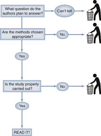
If an interesting question has been posed in a clearly assessable way and an appropriate method has been chosen to answer the question, it is worth delving into the details to determine whether the authors have carried out the study well and obtained a useful answer to their question. The details of understanding appropriate methodology and appropriate results are not difficult or terribly voluminous and are well within the capabilities of the practicing neurosurgeon to have a working knowledge sufficient for evaluating publications in the neurosurgical literature. According to a scheme first proposed by Sackett and colleagues, single therapeutic studies are classified into five levels according to the quality of the evidence.173 These categories are relevant to articles on therapeutic efficacy. Corresponding ratings for articles on diagnostic tests, prognosis, and review methodology remain to be developed. The single article on classification is shown in Table 11-9. The Centre for Evidence-Based Medicine at Oxford University maintains a detailed updated list of levels of evidence for both single studies and cumulative evidence at http://www.cebm.net/index.aspx?o=1025.
TABLE 11-9 Classification of Cumulative Evidence
| Evidentiary Classification of Levels of Evidence for Single Articles on Therapy173 |
Evaluating Cumulative Evidence
Accumulated evidence may also be summarized in a practice parameter development process. Many professional organizations have participated in the development of evidence-based practice parameters (sometimes called guidelines). When the principles of critical analysis, systematic review, and meta-analysis have been applied, true evidence-based practice parameters should result. Such practice parameters provide a tremendous time savings for the busy practitioner. Classification of cumulative evidence is also shown in Table 11-9 (see also http://www.cebm.net/index.aspx?o=1025).173 A few sources of practice parameters are shown in Table 11-10.174 The practitioner must be aware, however, that not all practice parameters are developed with evidence-based principles and that the methods used to develop the parameters must be reviewed if they are to be relied on. Excellent neurosurgical examples of evidence-based practice parameters can be found in the guidelines for the management of acute cervical spine and spinal cord injuries.89
Practice Assessment
The third stage of evidence-based practice is the implementation of ongoing outcome assessment.
Health functional status measurement instruments developed by the Foundation for Health Care Evaluation are available in paper and computerized form. These would allow SF-36 or SF-12 instruments to be collected on every patient. Some commercial outcome measurement systems are available, and some states have developed outcome monitoring instruments (e.g., http://www.rand.org/health/surveys/sf36item/ and http://www.qualitymetric.com).
Aldape K, Simmons ML, Davis RL, et al. Discrepancies in diagnoses of neuroepithelial neoplasms: the San Francisco Bay Area Adult Glioma Study. Cancer. 2000;88:2342.
Barker FGII, Curry WTJr, Carter BS. Surgery for primary supratentorial brain tumors in the United States, 1988 to 2000: the effect of provider caseload and centralization of care. Neuro Oncol. 2005;7:49.
Bhandari M, Devereaux PJ, Montori V, et al. Users’ guide to the surgical literature: how to use a systematic literature review and meta-analysis. Can J Surg. 2004;47:60.
Blettner M, Sauerbrei W, Schlehofer B, et al. Traditional reviews, meta-analyses and pooled analyses in epidemiology. Int J Epidemiol. 1999;28:1.
Davis FG, McCarthy BJ, Berger MS. Centralized databases available for describing primary brain tumor incidence, survival, and treatment: Central Brain Tumor Registry of the United States; Surveillance, Epidemiology, and End Results; and National Cancer Data Base. Neuro Oncol. 1999;1:205.
Gerszten PC. Outcomes research: a review. Neurosurgery. 1998;43:1146.
Haines S, Walters B. Evidence-Based Neurosurgery: An Introduction. New York: Thieme; 2006.
Haynes RB, Sackett DL, Guyatt GH, et al. Clinical Epidemiology. How To Do Clinical Practice Research, 3rd ed. Philadelphia: Lippincott Williams & Wilkins; 2006.
Lefebvre C, Clarke M. Identifying randomised trials. In: Egger M, vey Smith G, Altman D, editors. Systematic Reviews in Health Care: Meta-analysis in Context. 2nd ed. London: BMJ; 2001:69.
Pollock BE. Guiding Neurosurgery by Evidence. Basel: Karger; 2006.
Thompson SG, Sharp SJ. Explaining heterogeneity in meta-analysis: a comparison of methods. Stat Med. 1999;18:2693.
, 1998 Unruptured intracranial aneurysms—risk of rupture and risks of surgical intervention. International Study of Unruptured Intracranial Aneurysms Investigators [published erratum appears in N Engl J Med. 1999;340(9):744]. N Engl J Med. 1998;339:1725.
1 Sackett DL. Bias in analytic research. J Chronic Dis. 1979;32:51.
2 Freiman JA, Chalmers TC, Smith HJr, et al. The importance of beta, the type II error and sample size in the design and interpretation of the randomized control trial. Survey of 71 “negative” trials. N Engl J Med. 1978;299:690.
3 Haines SJ, Walters BC. Proof of equivalence. The inference of statistical significance. “Caveat emptor” [editorial]. Neurosurgery. 1993;33:432.
4 Detsky AS, Sackett DL. When was a “negative” clinical trial big enough? How many patients you needed depends on what you found. Arch Intern Med. 1985;145:709.
5 Goodman SN, Berlin JA. The use of predicted confidence intervals when planning experiments and the misuse of power when interpreting results. Ann Intern Med. 1994;121:200.
6 Drake JM, Kestle JR, Milner R, et al. Randomized trial of cerebrospinal fluid shunt valve design in pediatric hydrocephalus. Neurosurgery. 1998;43:294.
7 Haynes RB, Sackett DL, Guyatt GH, et al. Clinical Epidemiology. How To Do Clinical Practice Research, 3rd ed. Philadephia: Lippincott Williams & Wilkins; 2006.
8 Tuli S, Drake J, Lawless J, et al. Risk factors for repeated cerebrospinal shunt failures in pediatric patients with hydrocephalus. J Neurosurg. 2000;92:31.
9 Deyo RA, Rainville J, Kent DL. What can the history and physical examination tell us about low back pain? JAMA. 1992;268:760.
10 Pewsner D, Battaglia M, Minder C, et al. Ruling a diagnosis in or out with “SpPIn” and “SnNOut”: a note of caution. BMJ. 2004;329:209.
11 Bederson JB, Awad IA, Wiebers DO, et al. Recommendations for the management of patients with unruptured intracranial aneurysms: a statement for healthcare professionals from the stroke council of the American Heart Association. Stroke. 2000;31:2742.
12 Steinbok P, Boyd M, Flodmark CO, et al. Radiographic imaging requirements following ventriculoperitoneal shunt procedures. Pediatr Neurosurg. 1995;22:141.
13 Brockmeyer D. Down syndrome and craniovertebral instability. Topic review and treatment recommendations. Pediatr Neurosurg. 1999;31:71.
14 Stiell IG, Wells GA, Vandemheen KL, et al. The Canadian C-spine rule for radiography in alert and stable trauma patients. JAMA. 2001;286:1841.
15 Hoffman JR, Mower WR, Wolfson AB, et al. Validity of a set of clinical criteria to rule out injury to the cervical spine in patients with blunt trauma. National Emergency X-Radiography Utilization Study Group. N Engl J Med. 2000;343:94.
16 Fagan TJ. Nomogram for Bayes theorem [letter]. N Engl J Med. 1975;293:257.
17 Jaeschke R, Guyatt GH, Sackett DL. Users’ guides to the medical literature. III. How to use an article about a diagnostic test. B. What are the results and will they help me in caring for my patients? The Evidence-Based Medicine Working Group. JAMA. 1994;271:703.
18 Jaeschke R, Guyatt G, Sackett DL. Users’ guides to the medical literature. III. How to use an article about a diagnostic test. A. Are the results of the study valid? Evidence-Based Medicine Working Group. JAMA. 1994;271:389.
19 Vroomen PC, de Krom MC, Knottnerus JA. Diagnostic value of history and physical examination in patients suspected of sciatica due to disc herniation: a systematic review. J Neurol. 1999;246:899.
20 Levin BE. The clinical significance of spontaneous pulsations of the retinal vein. Arch Neurol. 1978;35:37.
21 Tuite GF, Chong WK, Evanson J, et al. The effectiveness of papilledema as an indicator of raised intracranial pressure in children with craniosynostosis. Neurosurgery. 1996;38:272.
22 Piatt JHJr. Physical examination of patients with cerebrospinal fluid shunts: is there useful information in pumping the shunt? Pediatrics. 1992;89:470.
23 Johnson DL, Conry J, O’Donnell R. Epileptic seizure as a sign of cerebrospinal fluid shunt malfunction. Pediatr Neurosurg. 1996;24:223.
24 Garton HJ, Kestle JR, Drake JM. Predicting shunt failure on the basis of clinical symptoms and signs in children. J Neurosurg. 2001;94:202.
25 Streiner D, Norman G. Health Measurement Scales: A Practical Guide to Their Development and Use, 2nd ed. Oxford: Oxford University Press; 1995.
26 Gerszten PC. Outcomes research: a review. Neurosurgery. 1998;43:1146.
27 Hamilton BB, Laughlin JA, Fiedler RC, et al. Interrater reliability of the 7-level functional independence measure (FIM). Scand J Rehabil Med. 1994;26:115.
28 Guyatt GH, Feeny DH, Patrick DL. Measuring health-related quality of life. Ann Intern Med. 1993;118:622.
29 Shrout P, Fleiss J. Intraclass correlations: uses in assessing rater reliability. Psychol Bull. 1979;86:420.
30 Fleiss J, Levin B, Park M. Statistical Methods for Rates and Proportions. New York: John Wiley; 2004.
31 Cronbach LJ. Coefficient alpha and the internal structure of tests. Psychometrika. 1951;16:297.
32 Cohen J. A coefficient of agreement for nominal scales. Educ Psychol Meas. 1960;20:37.
33 Cohen J. Weighted kappa: nominal scale agreement with provision for scaled disagreement of partial credit. Psychol Bull. 1968;70:213.
34 Landis JR, Koch GG. The measurement of observer agreement for categorical data. Biometrics. 1977;33:159.
35 Kestle J, Milner R, Drake J. The shunt design trial: variation in surgical experience did not influence shunt survival. Pediatr Neurosurg. 1999;30:283.
36 Guggenmoos-Holzmann I. How reliable are chance-corrected measures of agreement? Stat Med. 1993;12:2191.
37 Guggenmoos-Holzmann I. The meaning of kappa: probabilistic concepts of reliability and validity revisited. J Clin Epidemiol. 1996;49:775.
38 Bracken MB, Shepard MJ, Holford TR, et al. Administration of methylprednisolone for 24 or 48 hours or tirilazad mesylate for 48 hours in the treatment of acute spinal cord injury. Results of the Third National Acute Spinal Cord Injury Randomized Controlled Trial. National Acute Spinal Cord Injury Study. JAMA. 1997;277:1597.
39 Bracken MB, Shepard MJ, Collins WF, et al. A randomized, controlled trial of methylprednisolone or naloxone in the treatment of acute spinal-cord injury. Results of the Second National Acute Spinal Cord Injury Study. N Engl J Med. 1990;322:1405.
40 Bracken MB, Collins WF, Freeman DF, et al. Efficacy of methylprednisolone in acute spinal cord injury. JAMA. 1984;251:45.
41 Molloy S, Price M, Casey AT. Questionnaire survey of the views of the delegates at the European Cervical Spine Research Society meeting on the administration of methylprednisolone for acute traumatic spinal cord injury. Spine. 2001;26:E562.
42 Nesathurai S. Steroids and spinal cord injury: revisiting the NASCIS 2 and NASCIS 3 trials. J Trauma. 1998;45:1088.
43 Hurlbert RJ. Methylprednisolone for acute spinal cord injury: an inappropriate standard of care. J Neurosurg. 2000;93:1.
44 Teasdale G, Jennett B. Assessment of coma and impaired consciousness. A practical scale. Lancet. 1974;2:81.
45 Jennett B, Bond M. Assessment of outcome after severe brain damage. Lancet. 1975;1:480.
46 Rappaport M, Hall KM, Hopkins K, et al. Disability rating scale for severe head trauma: coma to community. Arch Phys Med Rehabil. 1982;63:118.
47 Hagen C, Malkmus D, Durham P. Measures of Cognitive Functioning in the Rehabilitation Facility. Brain Injury Association. 1984.
48 Cockrell J, Folstein M. Mini-Mental State Examination (MMSE). Psychopharmocol Bull. 1988;24:689.
49 Folstein M, Folstein S, McHugh P. “Mini-mental state.” A practical method for grading the cognitive state of patients for the clinician. J Psychiatr Res. 1975;12:189.
50 Bowling A. Measuring Disease, 2nd ed. Buckingham: Open University Press; 2001.
51 Wechsler D. WAIS-R Manual: Wechsler Adult Intelligence Scale, revised ed. New York: Psychological Corporation; 1981.
52 Engel J. Outcome with respect to epileptic seizures. In: Engle J, editor. Surgical Treatment of the Epilepsies. New York: Raven Press; 1987:5531.
53 Fahn S, Elton RL, members of the UPDRS Development Committee. Unified Parkinson’s Disease Rating Scale. In: Fahn S, Marsden CD, Goldstein M, et al, editors. Recent Developments in Parkinson’s Disease, Vol. 2. Florham Park, NJ: McMillan; 1987:153.
54 Ashworth B. Preliminary trail of carisoprodol in multiple sclerosis. Practitioner. 1964;192:540.
55 Hunt WE, Hess RM. Surgical risk as related to time of intervention in the repair of intracranial aneurysms. J Neurosurg. 1968;28:14.
56 Hunt WE, Kosnik EJ. Timing and perioperative care in intracranial aneurysm surgery. Clin Neurosurg. 1974;21:79.
57 Drake CG. Report of World Federation of Neurological Surgeons Committee on a Universal Subarachnoid Hemorrhage Grading Scale. J Neurosurg. 1988;68:985.
58 Brott T, Adams HPJr, Olinger CP, et al. Measurements of acute cerebral infarction: a clinical examination scale. Stroke. 1989;20:864.
59 Ranklin J. Cerebral vascular accidents in patients over the age of 60. II: Prognosis. Scott Med J. 1957;2:200.
60 United Kingdom transient ischaemic attack (UK-TIA) aspirin trial: interim results. UK-TIA Study Group. BMJ. 1988;296:316.
61 House JW, Brackmann DE. Facial nerve grading system. Otolaryngol Head Neck Surg. 1985;93:146.
62 Maynard FMJr, Bracken MB, Creasey G, et al. International standards for neurological and functional classification of spinal cord injury. American Spinal Injury Association. Spinal Cord. 1997;35:266.
63 Frankel HL, Hancock DO, Hyslop G, et al. The value of postural reduction in the initial management of closed injuries of the spine with paraplegia and tetraplegia. I. Paraplegia. 1969;7:179.
64 Medical Research Council. Aids to Examination of the Peripheral Nervous System. Memorandum No. 45. London: HMSO; 1976.
65 Hunsaker FG, Cioffi DA, Amadio PC, et al. The American Academy of Orthopaedic Surgeons outcomes instruments: normative values from the general population. J Bone Joint Surg Am. 2002;84:208.
66 Fairbank JC, Couper J, Davies JB, et al. The Oswestry low back pain disability questionnaire. Physiotherapy. 1980;66:271.
67 Jamjoom A, Williams C, Cummins B. The treatment of spondylotic cervical myelopathy by multiple subtotal vertebrectomy and fusion. Br J Neurosurg. 1991;5:249.
68 Kulkarni AV, Drake JM, Rabin D, et al. Measuring the health status of children with hydrocephalus by using a new outcome measure. J Neurosurg. 2004;101:141.
69 Kulkarni AV, Rabin D, Drake JM. An instrument to measure the health status in children with hydrocephalus: the Hydrocephalus Outcome Questionnaire. J Neurosurg. 2004;101:134.
70 Whitaker LA, Bartlett SP, Schut L, et al. Craniosynostosis: an analysis of the timing, treatment, and complications in 164 consecutive patients. Plast Reconstr Surg. 1987;80:195.
71 Karnofsky D, Burchenal J. The clinical evaluation of chemotherapy agents in cancer. In: Macleod CM, editor. Evaluation of Chemotherapy Agents. New York: Columbia University Press; 1949:191.
72 Bampoe J, Laperriere N, Pintilie M, et al. Quality of life in patients with glioblastoma multiforme participating in a randomized study of brachytherapy as a boost treatment. J Neurosurg. 2000;93:917.
73 Kiebert GM, Curran D, Aaronson NK, et al. Quality of life after radiation therapy of cerebral low-grade gliomas of the adult: results of a randomised phase III trial on dose response (EORTC trial 22844). EORTC Radiotherapy Co-operative Group. Eur J Cancer. 1998;34:1902.
74 Granger CV, Hamilton BB, Keith RA, et al. Advances in functional assessment for medical rehabilitation. Top Geriatr Rehabil. 1986;1:59.
75 Msall ME, DiGaudio K, Duffy LC, et al. WeeFIM. Normative sample of an instrument for tracking functional independence in children. Clin Pediatr (Phila). 1994;33:431.
76 Msall ME, DiGaudio K, Rogers BT, et al. The Functional Independence Measure for Children (WeeFIM). Conceptual basis and pilot use in children with developmental disabilities. Clin Pediatr (Phila). 1994;33:421.
77 Mahoney FI, Barthel DW. Functional evaluation: the Barthel Index. Md State Med J. 1965;14:62.
78 Collin C, Wade DT, Davies S, et al. The Barthel ADL Index: a reliability study. Int Disabil Stud. 1988;10:61.
79 Melzack R. The McGill Pain Questionnaire: major properties and scoring methods. Pain. 1975;1:277.
80 Huskisson EC. Measurement of pain. Lancet. 1974;2:1127.
81 Ware JEJr, Sherbourne CD. The MOS 36-item short-form health survey (SF-36). I. Conceptual framework and item selection. Med Care. 1992;30:473.
82 Bergner M, Bobbitt RA, Carter WB, et al. The Sickness Impact Profile: development and final revision of a health status measure. Med Care. 1981;19:787.
83 Hunt SM, McEwen J, McKenna SP. Measuring health status: a new tool for clinicians and epidemiologists. J R Coll Gen Pract. 1985;35:185.
84 McKenna S, Hunt S, Tennant A. The development of a patient-completed index of distress from the Nottingham health profile: a new measure for use in cost-utility studies. Br J Med Econ. 1993;6:13.
85 McDowell I, Newell C. Measuring Health, 2nd ed. New York: Oxford University Press; 1996.
86 World Health Organization. Constitution of the World Health Organization. WHO Chron. 1947;1:29.
87 Walters B. Measuring treatment success: outcome assessments in neurological surgery. In: Crockard A, Hayward RD, Hoff JT, editors. Neurosurgery: The Scientific Basis of Medical Practice, Vol 2. Oxford: Blackwell Scientific; 2000:12707.
88 Bampoe J, Ritvo P, Bernstein M. Quality of Life in patients with brain tumor: what’s relevant in our quest for therapeutic efficacy. Neurosurg Focus. 1998;4(6):e6.
89 AANS/CNS Joint section on Disorders of the Spine and Peripheral Nerves Guidelines Committee. Clinical assessment after acute cervical spinal cord injury. Neurosurgery. 2002;50:S21.
90 Hennekens C, Buring J. Epidemiology in Medicine. Boston: Little, Brown; 1987.
91 Marshall M, Lockwood A, Bradley C, et al. Unpublished rating scales: a major source of bias in randomised controlled trials of treatments for schizophrenia. Br J Psychiatry. 2000;176:249.
92 Flinn WR, Sandager GP, Cerullo LJ, et al. Duplex venous scanning for the prospective surveillance of perioperative venous thrombosis. Arch Surg. 1989;124:901.
93 Unruptured intracranial aneurysms—risk of rupture and risks of surgical intervention. International Study of Unruptured Intracranial Aneurysms Investigators [published erratum appears in N Engl J Med. 1999;340(9):744]. N Engl J Med. 1998;339:1725.
94 Wiebers DO, Whisnant JP, Huston J3rd, et al. Unruptured intracranial aneurysms: natural history, clinical outcome, and risks of surgical and endovascular treatment. Lancet. 2003;362:103.
95 Juvela S, Porras M, Heiskanen O. Natural history of unruptured intracranial aneurysms: a long-term follow-up study. J Neurosurg. 1993;79:174.
96 Juvela S, Porras M, Poussa K. Natural history of unruptured intracranial aneurysms: probability of and risk factors for aneurysm rupture. J Neurosurg. 2000;93:379.
97 Chang SM, Parney IF, Huang W, et al. Patterns of care for adults with newly diagnosed malignant glioma. JAMA. 2005;293:557.
98 Tu JV, Wang H, Bowyer B, et al. Risk factors for death or stroke after carotid endarterectomy: observations from the Ontario Carotid Endarterectomy Registry. Stroke. 2003;34:2568.
99 Khuri SF. The NSQIP: a new frontier in surgery. Surgery. 2005;138:837.
100 Davis FG, McCarthy BJ, Berger MS. Centralized databases available for describing primary brain tumor incidence, survival, and treatment: Central Brain Tumor Registry of the United States; Surveillance, Epidemiology, and End Results; and National Cancer Data Base. Neuro Oncol. 1999;1:205.
101 Wisoff JH, Boyett JM, Berger MS, et al. Current neurosurgical management and the impact of the extent of resection in the treatment of malignant gliomas of childhood: a report of the Children’s Cancer Group trial no. CCG-945. J Neurosurg. 1998;89:52.
102 Albright AL, Sposto R, Holmes E, et al. Correlation of neurosurgical subspecialization with outcomes in children with malignant brain tumors. Neurosurgery. 2000;47:879.
103 Steiner C, Elixhauser A, Schnaier J. The healthcare cost and utilization project: an overview. Eff Clin Pract. 2002;5:143.
104 Cooper GS, Virnig B, Klabunde CN, et al. Use of SEER-Medicare data for measuring cancer surgery. Med Care. 2002;40(8 suppl):IV-43.
105 Benesch C, Witter DMJr, Wilder AL, et al. Inaccuracy of the International Classification of Diseases (ICD-9-CM) in identifying the diagnosis of ischemic cerebrovascular disease. Neurology. 1997;49:660.
106 Aldape K, Simmons ML, Davis RL, et al. Discrepancies in diagnoses of neuroepithelial neoplasms: the San Francisco Bay Area Adult Glioma Study. Cancer. 2000;88:2342.
107 Davis FG, Malmer BS, Aldape K, et al. Issues of diagnostic review in brain tumor studies: from the Brain Tumor Epidemiology Consortium. Cancer Epidemiol Biomarkers Prev. 2008;17:484.
108 Best WR, Khuri SF, Phelan M, et al. Identifying patient preoperative risk factors and postoperative adverse events in administrative databases: results from the Department of Veterans Affairs National Surgical Quality Improvement Program. J Am Coll Surg. 2002;194:257.
109 Birkmeyer JD, Sharp SM, Finlayson SR, et al. Variation profiles of common surgical procedures. Surgery. 1998;124:917.
110 Barker FG2nd, Curry WTJr, Carter BS. Surgery for primary supratentorial brain tumors in the United States, 1988 to 2000: the effect of provider caseload and centralization of care. Neuro Oncol. 2005;7:49.
111 Hannan EL, Popp AJ, Feustel P, et al. Association of surgical specialty and processes of care with patient outcomes for carotid endarterectomy. Stroke. 2001;32:2890.
112 Smedley B, Stith A, Nelson A, editors. Unequal Treatment. Confronting Racial and Ethnic Disparities in Health Care. Washington, DC: Institute of Medicine, 2003.
113 Moher D, Schulz KF, Altman D. The CONSORT statement: revised recommendations for improving the quality of reports of parallel-group randomized trials. JAMA. 2001;285:1987.
114 Freeman TB, Vawter DE, Leaverton PE, et al. Use of placebo surgery in controlled trials of a cellular-based therapy for Parkinson’s disease. N Engl J Med. 1999;341:988.
115 Macklin R. The ethical problems with sham surgery in clinical research. N Engl J Med. 1999;341:992.
116 Spilker B. Guide to Clinical Trials. New York: Raven Press; 1991.
117 Bhandari M, Devereaux PJ, Montori V, et al. Users’ guide to the surgical literature: how to use a systematic literature review and meta-analysis. Can J Surg. 2004;47:60.
118 Steinberg KK, Smith SJ, Stroup DF, et al. Comparison of effect estimates from a meta-analysis of summary data from published studies and from a meta-analysis using individual patient data for ovarian cancer studies. Am J Epidemiol. 1997;145:917.
119 Berlin JA, Santanna J, Schmid CH, et al. Individual patient- versus group-level data meta-regressions for the investigation of treatment effect modifiers: ecological bias rears its ugly head. Stat Med. 2002;21:371.
120 Verhagen AP, de Vet HC, de Bie RA, et al. The art of quality assessment of RCTs included in systematic reviews. J Clin Epidemiol. 2001;54:651.
121 Jadad AR, Moore RA, Carroll D, et al. Assessing the quality of reports of randomized clinical trials: is blinding necessary? Control Clin Trials. 1996;17:1.
122 Slim K, Nini E, Forestier D, et al. Methodological index for non-randomized studies (minors): development and validation of a new instrument. Aust N Z J Surg. 2003;73:712.
123 Deeks JJ. Issues in the selection of a summary statistic for meta-analysis of clinical trials with binary outcomes. Stat Med. 2002;21:1575.
124 DerSimonian R, Laird N. Meta-analysis in clinical trials. Control Clin Trials. 1986;7:177.
125 Deeks J, Altman D, Bradburn M. Statistical methods for examining heterogeneity and combining results from several studies in meta-analysis. In Egger M, vey Smith G, Altman D, editors: Systematic Reviews in Health Care: Meta-analysis in Context, 2nd ed, London: BMJ, 2001.
126 Thompson SG, Sharp SJ. Explaining heterogeneity in meta-analysis: a comparison of methods. Stat Med. 1999;18:2693.
127 Thompson SG. Why sources of heterogeneity in meta-analysis should be investigated. BMJ. 1994;309:1351.
128 Oxman AD, Guyatt GH. Validation of an index of the quality of review articles. J Clin Epidemiol. 1991;44:1271.
129 Mulrow CD. The medical review article: state of the science. Ann Intern Med. 1987;106:485.
130 Bramwell VH, Williams CJ. Do authors of review articles use systematic methods to identify, assess and synthesize information? Ann Oncol. 1997;8:1185.
131 Blettner M, Sauerbrei W, Schlehofer B, et al. Traditional reviews, meta-analyses and pooled analyses in epidemiology. Int J Epidemiol. 1999;28:1.
132 Moher D, Tetzlaff J, Tricco AC, et al. Epidemiology and reporting characteristics of systematic reviews. PLoS Med. 2007;4:e78.
133 Lefebvre C, Clarke M. Identifying randomised trials. In: Egger M, vey Smith G, Altman D, editors. Systematic Reviews in Health Care: Meta-analysis in Context. 2nd ed. London: BMJ; 2001:69.
134 Begg CB. Comment on A comparison of methods to detect publication bias in meta-analysis by P. Macaskill, S. D. Walter and L. Irwig. Statistics in Medicine. 2001;20:641-654. Stat Med. 2002;21:1803; author reply 1804
135 Pham B, Platt R, McAuley L, et al. Is there a “best” way to detect and minimize publication bias? An empirical evaluation. Eval Health Prof. 2001;24:109.
136 van Limbeek J, Jacobs WC, Anderson PG, et al. A systematic literature review to identify the best method for a single level anterior cervical interbody fusion. Eur Spine J. 2000;9:129.
137 Metcalfe SE, Grant R. Biopsy versus resection for malignant glioma. Cochrane Database Syst Rev. 2001;3:CD002034.
138 Schierhout G, Roberts I. The Cochrane Brain and Spinal Cord Injury Group. J Neurol Neurosurg Psychiatry. 1997;63:1.
139 Levin A. The Cochrane Collaboration. Ann Intern Med. 2001;135:309.
140 Bombardier C, Esmail R, Nachemson AL. The Cochrane Collaboration Back Review Group for spinal disorders. Spine. 1997;22:837.
141 Counsell C, Warlow C, Sandercock P, et al. The Cochrane Collaboration Stroke Review Group. Meeting the need for systematic reviews in stroke care. Stroke. 1995;26:498.
142 Bero L, Rennie D. The Cochrane Collaboration. Preparing, maintaining, and disseminating systematic reviews of the effects of health care. JAMA. 1995;274:1935.
143 Haines S, Walters B. Evidence-Based Neurosurgery: An Introduction. New York: Thieme; 2006.
144 Haines SJ. Evidence-based neurosurgery. Neurosurgery. 2003;52:36.
145 Guyatt GH, Sackett DL, Cook DJ. Users’ guides to the medical literature. II. How to use an article about therapy or prevention. A. Are the results of the study valid? Evidence-Based Medicine Working Group. JAMA. 1993;270:2598.
146 Richardson WS, Wilson MC, Williams JWJr, et al. Users’ guides to the medical literature: XXIV. How to use an article on the clinical manifestations of disease. Evidence-Based Medicine Working Group. JAMA. 2000;284:869.
147 Oxman AD, Sackett DL, Guyatt GH. Users’ guides to the medical literature. I. How to get started. Evidence-Based Medicine Working Group. JAMA. 1993;270:2093.
148 Guyatt GH, Sackett DL, Cook DJ. Users’ guides to the medical literature. II. How to use an article about therapy or prevention. B. What were the results and will they help me in caring for my patients? Evidence-Based Medicine Working Group. JAMA. 1994;271:59.
149 Laupacis A, Wells G, Richardson WS, et al. Users’ guides to the medical literature. V. How to use an article about prognosis. Evidence-Based Medicine Working Group. JAMA. 1994;272:234.
150 Levine M, Walter S, Lee H, et al. Users’ guides to the medical literature. IV. How to use an article about harm. Evidence-Based Medicine Working Group. JAMA. 1994;271:1615.
151 Oxman AD, Cook DJ, Guyatt GH. Users’ guides to the medical literature. VI. How to use an overview. Evidence-Based Medicine Working Group. JAMA. 1994;272:1367.
152 Guyatt GH, Sackett DL, Sinclair JC, et al. Users’ guides to the medical literature. IX. A method for grading health care recommendations. Evidence-Based Medicine Working Group [published erratum appears in JAMA. 1996;275(16):1232]. JAMA. 1995;274:1800.
153 Hayward RS, Wilson MC, Tunis SR, et al. Users’ guides to the medical literature. VIII. How to use clinical practice guidelines. A. Are the recommendations valid? The Evidence-Based Medicine Working Group. JAMA. 1995;274:570.
154 Wilson MC, Hayward RS, Tunis SR, et al. Users’ guides to the medical literature. VIII. How to use clinical practice guidelines. B. What are the recommendations and will they help you in caring for your patients? Evidence-Based Medicine Working Group. JAMA. 1995;274:1630.
155 Naylor CD, Guyatt GH. Users’ guides to the medical literature. XI. How to use an article about a clinical utilization review. Evidence-Based Medicine Working Group. JAMA. 1996;275:1435.
156 Drummond MF, Richardson WS, O’Brien BJ, et al. Users’ guides to the medical literature. XIII. How to use an article on economic analysis of clinical practice. A. Are the results of the study valid? Evidence-Based Medicine Working Group. JAMA. 1997;277:1552.
157 Guyatt GH, Naylor CD, Juniper E, et al. Users’ guides to the medical literature. XII. How to use articles about health-related quality of life. Evidence-Based Medicine Working Group. JAMA. 1997;277:1232.
158 O’Brien BJ, Heyland D, Richardson WS, et al. Users’ guides to the medical literature. XIII. How to use an article on economic analysis of clinical practice. B. What are the results and will they help me in caring for my patients? Evidence-Based Medicine Working Group [published erratum appears in JAMA. 1997;278(13):1064]. JAMA. 1997;277:1802.
159 Dans AL, Dans LF, Guyatt GH, et al. Users’ guides to the medical literature: XIV. How to decide on the applicability of clinical trial results to your patient. Evidence-Based Medicine Working Group. JAMA. 1998;279:545.
160 Barratt A, Irwig L, Glasziou P, et al. Users’ guides to the medical literature: XVII. How to use recommendations about screening. Evidence-Based Medicine Working Group. JAMA. 1999;281:2029.
161 Bucher HC, Guyatt GH, Cook DJ, et al. Users’ guides to the medical literature: XIX. Applying clinical results. A. How to use an article measuring the effect of an intervention on surrogate end points. Evidence-Based Medicine Working Group. JAMA. 1999;282:771.
162 Guyatt GH, Sinclair J, Cook DJ, et al. Users’ guides to the medical literature: XVI. How to use a recommendation. Evidence-Based Medicine Working Group and the Applicability Methods Working Group. JAMA. 1999;281:1836.
163 Randolph AG, Haynes RB, Wyatt JC, et al. Users’ guides to the medical literature: XVIII. How to use an article evaluating the clinical impact of a computer-based clinical decision support system. Evidence-Based Medicine Working Group. JAMA. 1999;282:67.
164 Richardson WS, Wilson MC, Guyatt GH, et al. Users’ guides to the medical literature: XV. How to use an article about disease probability for differential diagnosis. Evidence-Based Medicine Working Group. JAMA. 1999;281:1214.
165 Giacomini MK, Cook DJ. Users’ guides to the medical literature: XXIII. Qualitative health care B. What are the results and how do they help me care patients? Evidence-Based Medicine Working Group. JAMA. 2000;284:478.
166 Giacomini MK, Cook DJ. Users’ guides to the medical literature: XXIII. Qualitative health care A. Are the results of the study valid? Evidence-Based Medicine Working Group. JAMA. 2000;284:357.
167 Guyatt GH, Haynes RB, Jaeschke RZ, et al. Users’ guides to the medical literature: XXV. Evidence-based principles for applying the users’ guides to patient care. Evidence-Based Medicine Working Group. JAMA. 2000;284:1290.
168 Hunt DL, Jaeschke R, McKibbon KA. Users’ guides to the medical literature: XXI. Using electronic information resources in evidence-based practice. Evidence-Based Medicine Working Group. JAMA. 2000;283:1875.
169 McAlister FA, Straus SE, Guyatt GH, et al. Users’ guides to the medical literature: XX. Integrating research with the care of the individual patient. Evidence-Based Medicine Working Group. JAMA. 2000;283:2829.
170 McGinn TG, Guyatt GH, Wyer PC, et al. Users’ guides to the medical literature: XXII: how to use clinical decision rules. Evidence-Based Medicine Working Group. JAMA. 2000;284:79.
171 Rennie D. Users’ Guides to the Medical Literature: A Manual for Evidence-Based Clinical Practice. et al. New York: McGraw Hill. 2008.
172 Pollock BE. Guiding Neurosurgery by Evidence. Basel: Karger; 2006.
173 Sackett DL. Rules of evidence and clinical recommendations on the use of antithrombotic agents. Chest. 1989;95:2S.
174 Rosenberg J, Greenberg MK. Practice parameters: strategies for survival into the nineties. Neurology. 1992;42:1110.
Appendix
Critical Assessment of the Medical Literature
In an evidence-based approach to medicine, one attempts to generalize data from the medical literature to the specific clinical question at hand. Therefore, it is of great value to be able to critically assess the quality of the evidence provided therein. Given an understanding of the design features of the particular study types described in this chapter, a structure for systematically assessing individual publications becomes apparent. The following guidelines are in summary form and address only the common study methodologies identified earlier. The basic questions are Why?, How?, Who?, What?, How many?, and So what?1 Additional assistance with these methodologies, as well as others such as economic analyses, clinical decision analysis, and health services research, can be found through the “Users Guide to the Medical Literature” series that has appeared periodically during the past decade in the Journal of the American Medical Association2–28 and has recently been updated in book form.29
Why
The initial step is to define a study’s purpose or principal question. This should be clearly stated in the introduction or abstract. Sackett and colleagues offer these common clinical research questions relevant to both the designer and user of clinical research. Basic questions include the following30,31:
Each of these types of studies should then be assessed methodologically as follows.
Studies About Diagnosis
Who Is Being Studied and How?
What Is Being Studied?
How Has the Analysis Occurred?
Studies About Natural History
Who Is Being Studied?
What Is Being Studied?
How Has the Analysis Occurred?
Studies About Best Therapy
How Is the Study Conducted?
Who Are the Patients in the Study?
What Is Being Done to the Patients?
How Are the Results Analyzed?
1 Schechter MT, LeBlanc FE, Lawrence VA. Appraising new information. In: Tyroidl H, McKneally MF, Mulder DS, et al, editors. Surgical Research. New York: Springer-Verlag, 1998.
2 Jaeschke R, Guyatt G, Sackett DL. Users’ guides to the medical literature. III. How to use an article about a diagnostic test. A. Are the results of the study valid? Evidence-Based Medicine Working Group. JAMA. 1994;271:389.
3 Jaeschke R, Guyatt GH, Sackett DL. Users’ guides to the medical literature. III. How to use an article about a diagnostic test. B. What are the results and will they help me in caring for my patients? Evidence-Based Medicine Working Group. JAMA. 1994;271:703.
4 Guyatt GH, Sackett DL, Cook DJ. Users’ guides to the medical literature. II. How to use an article about therapy or prevention. A. Are the results of the study valid? Evidence-Based Medicine Working Group. JAMA. 1993;270:2598.
5 Richardson WS, Wilson MC, Williams JWJr, et al. Users’ guides to the medical literature: XXIV. How to use an article on the clinical manifestations of disease. Evidence-Based Medicine Working Group. JAMA. 2000;284:869.
6 Oxman AD, Sackett DL, Guyatt GH. Users’ guides to the medical literature. I. How to get started. Evidence-Based Medicine Working Group. JAMA. 1993;270:2093.
7 Guyatt GH, Sackett DL, Cook DJ. Users’ guides to the medical literature. II. How to use an article about therapy or prevention. B. What were the results and will they help me in caring for my patients? Evidence-Based Medicine Working Group. JAMA. 1994;271:59.
8 Laupacis A, Wells G, Richardson WS, et al. Users’ guides to the medical literature. V. How to use an article about prognosis. Evidence-Based Medicine Working Group. JAMA. 1994;272:234.
9 Levine M, Walter S, Lee H, et al. Users’ guides to the medical literature. IV. How to use an article about harm. Evidence-Based Medicine Working Group. JAMA. 1994;271:1615.
10 Oxman AD, Cook DJ, Guyatt GH. Users’ guides to the medical literature. VI. How to use an overview. Evidence-Based Medicine Working Group. JAMA. 1994;272:1367.
11 Guyatt GH, Sackett DL, Sinclair JC, et al. Users’ guides to the medical literature. IX. A method for grading health care recommendations. Evidence-Based Medicine Working Group. JAMA. 1995;274:1800.
12 Wilson MC, Hayward RS, Tunis SR, et al. Users’ guides to the medical literature. VIII. How to use clinical practice guidelines. B. What are the recommendations and will they help you in caring for your patients? Evidence-Based Medicine Working Group. JAMA. 1995;274:1630.
13 Naylor CD, Guyatt GH. Users’ guides to the medical literature. XI. How to use an article about a clinical utilization review. Evidence-Based Medicine Working Group. JAMA. 1996;275:1435.
14 Drummond MF, Richardson WS, O’Brien BJ, et al. Users’ guides to the medical literature. XIII. How to use an article on economic analysis of clinical practice. A. Are the results of the study valid? Evidence-Based Medicine Working Group. JAMA. 1997;277:1552.
15 Guyatt GH, Naylor CD, Juniper E, et al. Users’ guides to the medical literature. XII. How to use articles about health-related quality of life. Evidence-Based Medicine Working Group. JAMA. 1997;277:1232.
16 O’Brien BJ, Heyland D, Richardson WS, et al. Users’ guides to the medical literature. XIII. How to use an article on economic analysis of clinical practice. B. What are the results and will they help me in caring for my patients? Evidence-Based Medicine Working Group. JAMA. 1997;277:1802.
17 Dans AL, Dans LF, Guyatt GH, et al. Users’ guides to the medical literature: XIV. How to decide on the applicability of clinical trial results to your patient. Evidence-Based Medicine Working Group. JAMA. 1998;279:545.
18 Barratt A, Irwig L, Glasziou P, et al. Users’ guides to the medical literature: XVII. How to use guidelines and recommendations about screening. Evidence-Based Medicine Working Group. JAMA. 1999;281:2029.
19 Bucher HC, Guyatt GH, Cook DJ, et al. Users’ guides to the medical literature: XIX. Applying clinical trial results. A. How to use an article measuring the effect of an intervention on surrogate end points. Evidence-Based Medicine Working Group. JAMA. 1999;282:771.
20 Guyatt GH, Sinclair J, Cook DJ, et al. Users’ guides to the medical literature: XVI. How to use a treatment recommendation. Evidence-Based Medicine Working Group and the Cochrane Applicability Methods Working Group. JAMA. 1999;281:1836.
21 Randolph AG, Haynes RB, Wyatt JC, et al. Users’ guides to the medical literature: XVIII. How to use an article evaluating the clinical impact of a computer-based clinical decision support system. Evidence-Based Medicine Working Group. JAMA. 1999;282:67.
22 Richardson WS, Wilson MC, Guyatt GH, et al. Users’ guides to the medical literature: XV. How to use an article about disease probability for differential diagnosis. Evidence-Based Medicine Working Group. JAMA. 1999;281:1214.
23 Giacomini MK, Cook DJ. Users’ guides to the medical literature: XXIII. Qualitative research in health care A. Are the results of the study valid? Evidence-Based Medicine Working Group. JAMA. 2000;284:357.
24 Giacomini MK, Cook DJ. Users’ guides to the medical literature: XXIII. Qualitative research in health care B. What are the results and how do they help me care for my patients? Evidence-Based Medicine Working Group. JAMA. 2000;284:478.
25 Guyatt GH, Haynes RB, Jaeschke RZ, et al. Users’ guides to the medical literature: XXV. Evidence-based medicine: principles for applying the users’ guides to patient care. Evidence-Based Medicine Working Group. JAMA. 2000;284:1290.
26 Hunt DL, Jaeschke R, McKibbon KA. Users’ guides to the medical literature: XXI. Using electronic health information resources in evidence-based practice. Evidence-Based Medicine Working Group. JAMA. 2000;283:1875.
27 McAlister FA, Straus SE, Guyatt GH, et al. Users’ guides to the medical literature: XX. Integrating research evidence with the care of the individual patient. Evidence-Based Medicine Working Group. JAMA. 2000;283:2829.
28 McGinn TG, Guyatt GH, Wyer PC, et al. Users’ guides to the medical literature: XXII: how to use articles about clinical decision rules. Evidence-Based Medicine Working Group. JAMA. 2000;284:79.
29 Bero L, Rennie D. The Cochrane Collaboration: preparing, maintaining, and disseminating systematic reviews of the effects of health care. JAMA. 1995;274:1935.
30 Sackett DL, Haynes RB, Guyatt GH, et al. Clinical Epidemiology. A Basic Science for Clinical Medicine. Boston: Little, Brown; 1991.
31 Haynes RB, Sackett DL, Guyatt GH, et al. Clinical Epidemiology: How To Do Clinical Practice Research. Philadelphia: Lippincott Williams & Wilkins; 2006.
32 Feldman RD, Campbell N, Larochelle P, et al. 1999 Canadian recommendations for the management of hypertension. Task Force for the Development of the 1999 Canadian Recommendations for the Management of Hypertension. CMAJ. 1999;161(suppl 12):S1.