[level-membership-for-emergency-medicine-category]
218 Introduction to Cost-Effectiveness Analysis
 Key Points
• Cost-effectiveness analysis (CEA) is a method for evaluating and comparing the outcomes and costs of interventions designed to improve health.
• CEA is an increasingly important component of the medical literature because it drives both clinical and policy decisions that affect the practice of emergency medicine.
• The output of any CEA model is contingent on appropriate and accurate input data.
• The primary outcome of importance in a CEA is the incremental cost-effectiveness ratio, or ICER, which represents the incremental change in cost and effectiveness when choosing one strategy over another.
• CEA model outcomes incorporate a degree of uncertainty based on input data, which is quantified in the process of sensitivity analysis.
What Is Cost-Effectiveness Analysis?
A key skill for emergency physicians is effective integration of new interventions into existing clinical practice. Physicians have classically been trained and have become comfortable with more traditional methodologies of evaluating new interventions and treatment modalities, such as randomized controlled trials, but are often less comfortable in applying techniques such as cost-effectiveness analysis (CEA). As health care resources become more limited, costs rise, and treatment options expand, interventions and treatments are increasingly being compared and evaluated on the basis of cost.1
CEA falls under the broad umbrella of comparative effectiveness research, which refers to any study that compares the effectiveness of two or more strategies with or without regard to cost. CEA is a method for evaluating and comparing the outcomes and costs of interventions designed to improve health.2 Although many methodologies fall under the umbrella of CEA, they all share the common goal of reporting outcomes as a cost per achieving a unit of health effect (i.e., lives saved, year of life gained, quality-adjusted year of life gained). CEA tracks costs and effectiveness for a number of strategies by using both real and modeled data, compares the cost-effectiveness of the strategies, and then accounts for uncertainty in the data through sensitivity analyses.3
How Does Cost-Effectiveness Analysis Affect the Emergency Physician?
CEA is becoming an increasingly important input into health policy decisions; however, the methodology does have limitations. CEA cannot incorporate all aspects of a decision, and the results are only as good as the data available to input into the analyses. Economic analyses such as CEA cannot capture every input necessary to make health care decisions and should not be reported as scientific fact, but models and their results may be reported as aids in decision making.4 An additional criticism of CEA is that although the economic models have become increasingly complex to better represent reality, they have also become increasingly opaque to the lay reader, thus making it difficult for those without a background in economics to personally interpret the results.1 Despite these limitations, CEA offers the benefit of adding perspective to difficult questions regarding treatment choices in the setting of limited resources.2,5,6 If emergency physicians are to act as decision makers in our changing practice environment, it is essential to have an understanding of the basic principles of CEA.
Methodology in Cost-Effectiveness Analysis
Inputs
Perspective
Although one can perform a CEA from a vast number of perspectives, the most common is the societal perspective, which will be used for our example. In a CEA conducted from the societal perspective, the analyst considers all parties affected by the intervention and all costs related to the intervention, regardless of who experiences these costs and effects. Because the societal perspective includes all costs and health effects, it does not necessarily give an individual group the information necessary to make decisions on which interventions to implement. However, the societal perspective is used most commonly because it has several benefits.3 It is standardized and therefore allows comparison of various interventions across a broad spectrum of disciplines in medicine and society when making policy decisions. It is fair: if all decisions in health care were made from a societal standpoint, resources would be allocated to provide the most benefit to the most people. Moreover, although other perspectives may be more useful for individual groups, these perspectives do not necessarily take into account the cost or harm seen by those outside the sphere of the analyst’s perspective that the societal perspective takes into account.
Effectiveness
In CEA, each strategy has an associated effectiveness. The effectiveness (sometimes referred to in the economic literature as utility) can be expressed with a number of different metrics. The most common measure is “life-years gained” or “lives saved.” Traditionally, most medical and public health studies use “life-years,” whereas CEAs in transportation and environmental policy use “lives saved.”7
Even though life-years may be used alone as an effectiveness measure, they are generally adjusted to account for quality of life or disability. Without adjustment, two interventions would have the same effectiveness based on life-years even if one substantially increased quality of life without any extension in life expectancy. The most common adjustment unit is the quality-adjusted life-year (QALY), although other units such as disability-adjusted life-year are sometimes used.8
Discounting
An important aspect of economic analyses is the practice of discounting. Many CEAs take into account costs and health states that occur years in the future from the time of an intervention. To compare future costs and utilities with those occurring in the present, future costs and utilities are devalued at a constant yearly rate to reflect their lower opportunity cost. For example, if one needs to pay for a health intervention, clearly it is preferable to pay the same sum of money 10 years from now rather than paying today because the sum of money used for payment in the future could be invested in the meantime to generate further revenue. Therefore, a discount rate is applied to compare present and future events. The discount rate for all costs and utilities is generally approximately 3% to 5% per year in health economic analyses. Even though this value is commonly used, there is little agreement among economists regarding what represents an appropriate discount rate and exactly how this rate should be calculated.9,10
The Model
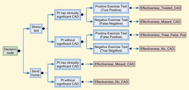
Mathematic models are used in CEA to simulate the chain of events surrounding alternative interventions so that the costs and outcomes related to the choice of one medical intervention over another can be tracked. Although it is theoretically possible to complete a CEA by measuring every variable prospectively, the broad scope of most CEAs necessitates at least some component of mathematic modeling.11,12 A successful model is transparent, internally consistent, reproducible, and interpretable.13 Multiple modeling methodologies are used in modern CEAs; here we will cover the two most common: decision tress and Markov models. Decision trees depict decisions and chance events as branches of a tree. Computerized decision trees can track the costs and outcomes associated with various health interventions. Graphic branches in the tree represent a chain of related events, and nodes in the branches represent decisions, such as a choice between competing strategies, or chances, such as the chance of a complication developing after an intervention. Figure 218.1 depicts a simple decision tree.
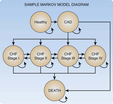
Certain situations are difficult to model with decision trees alone; especially problematic are episodic or recursive disease states (i.e., a chronic disease with frequent exacerbations). For these situations more complex models, such as Markov models, are used. A Markov model consists of a set of health states, as well as allowable transitions between these states. The model moves forward with discrete steps in time; at each time step the model allows patients to transition between states along allowable transitions according to predefined transition probabilities. Markov models can be constructed independently or be inserted into decision trees. If in our example CEA we wish to model CAD in more detail and specifically include ischemic congestive heart failure states, we could use a Markov model as depicted in Figure 218.2.
Primary Outcomes
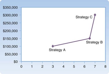
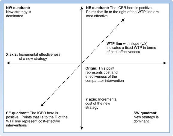
The most basic outcome from any CEA is a cost-effectiveness ratio (CE ratio), in which the cost of an intervention is placed in the numerator and the measure of effectiveness in the denominator; for instance, “dollars per QALY.” The CE ratio can then be compared with a predetermined “willingness to pay” to determine whether the intervention is cost-effective. Frequently, from a societal perspective a CE ratio is not particularly useful by itself because it involves a large number of societal costs and outcomes. It is often more useful to view the cost-effectiveness of one intervention versus another. The cost-effectiveness frontier graphically shows this difference, with cost on the y-axis and effectiveness on the x-axis (Fig. 218.3). To numerically compare two strategies, we use the incremental cost-effectiveness ratio (ICER). The ICER represents the incremental change in cost and effectiveness when choosing one strategy over another. For example, if the ICER for strategy A versus strategy B is $10 per QALY, by choosing to implement strategy A over strategy B, an additional $10 is spent for one additional QALY. A strategy is said to be dominant if it is both less costly and more effective than the comparator strategy. When interpreting ICERs it is important to remember two key points. First, the ICER is only as good as the value of the comparators. One can always make a strategy look good by comparing it with something bad. Second, ICERs should be reported only when positive. A negative ICER can mean one of two opposite scenarios: the new strategy is dominant, or the new strategy is dominated (more costly and less effective). The cost-effectiveness plane may be used as an intuitive way to understand and report ICERs between two strategies14 (Fig. 218.4).
Sensitivity Analyses
The point estimate of cost-effectiveness provided from a model is known as the “base case.”15 There is likely to be some uncertainty associated with the inputs of any model, and expressing this uncertainty in the outcome is a critical component of any CEA.9,12 The degree to which a model’s outcome changes with changes in particular inputs is referred to as its sensitivity. Examination of uncertainty in a CEA consists of varying input parameters and measuring the effects on results through sensitivity analyses. Sensitivity can be calculated on a number of levels.
 Facts and Formulas
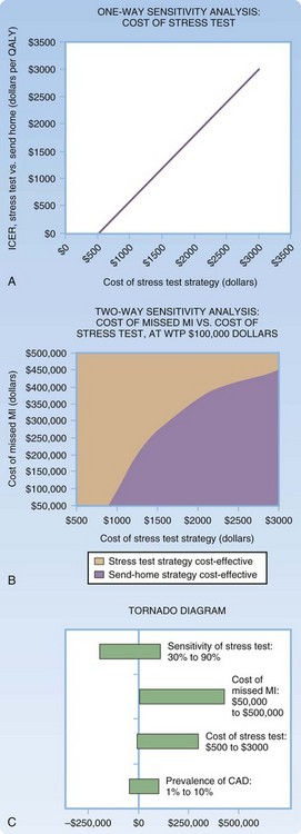
Sensitivity analyses may be reported as a threshold value (i.e., a threshold value on an input beyond which the intervention is cost-effective) or continuously, in which the resultant cost-effectiveness is considered across a range of input values.16 A one-way sensitivity analysis is the most basic form of sensitivity analysis. It demonstrates the variability in cost-effectiveness of an intervention or group of interventions based on variation of a single input. A two-way sensitivity analysis varies two variables simultaneously to capture their interaction. Any number of parameters can be varied simultaneously, although it is challenging to graphically depict sensitivity analyses beyond two way. Figure 218.5 depicts examples of one- and two-way sensitivity analyses for our example model, as well as an example of a tornado diagram, another commonly used methodology for reporting sensitivity. Tornado diagrams give a graphic representation of the magnitude of a number of one-way sensitivity analyses simultaneously but do not incorporate interaction between these variables.
The goal of multivariate sensitivity analysis is to gain a sense of model uncertainty by varying all variables simultaneously. It allows the generation of true confidence intervals of the inputs. The confidence interval for an ICER is dependent on the confidence intervals of all model inputs, as well as the structure of the model. Several methods have been described for empiric calculation of confidence intervals, but there is no consensus method. Most commonly, “bootstrap methods” are used, in which iterative methods are used to create confidence intervals from the data after the model has been run.17
The most common bootstrap method for calculating multivariate sensitivity is the Monte Carlo method. In a Monte Carlo analysis, each input in a model is replaced by a distribution representing the uncertainty surrounding the input variable. For instance, in our sample decision tree we may know that the incidence of CAD in the patient population in question is 0.1, with a 95% confidence interval of 0.05 to 0.15, normally distributed. To perform a Monte Carlo sensitivity analysis, we would replace our incidence point probability with a normal distribution of probabilities with a mean of 0.1 and standard deviation of 0.025. We would perform a similar replacement for all model inputs with uncertainty. The model would then be run many times (generally at least 1000).17 For each iteration of the model, the computer picks a value for each input based on the probability distribution. In the case of our CAD incidence distribution, most iterations would have values near the mean of 0.1, but some iterations would pick outlier values such that over the course of 1000 runs, the values picked would form the distribution specified. Each model run creates an individual ICER. These ICERs then form a distribution, the characteristics of which (standard deviation and confidence intervals) reflect the uncertainty of the model as whole.
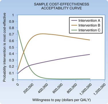
Several methods can be used for reporting confidence intervals generated from multivariate sensitivity analyses. In an ICE scatterplot (Fig. 218.6), individual runs of a multivariate Monte Carlo analysis are plotted as individual points on a cost-effectiveness plane.18 Figure 218.7 shows a sample cost-effectiveness acceptability curve in which individual model runs are compiled to form a probability distribution that reflects the likelihood that a given intervention is cost-effective at a given willingness to pay.17
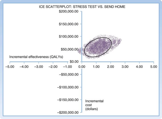
Fig. 218.6 Monte-Carlo sensitivity analysis: ICE scatterplot.
ICE, Incremental cost-effectiveness; QALYs, quality-adjusted life years.
Evaluating a Cost-Effectiveness Analysis
See Box 218.1 for a sample approach to critically evaluating a CEA. Though not the only approach or an all-inclusive list, it provides a framework for assessing the impact of a particular study on a clinical question. See “Suggested Readings” for more in-depth analysis.12,19–22
Box 218.1 Template for Critiquing a Cost-Effectiveness Analysis
1. What is the research question being asked?
2. What is the quality of the evidence?
3. Is the model’s design valid?
4. Are the base case results presented?
Black WC. The CE plane: a graphic representation of cost-effectiveness. Med Decis Making. 1990;10:212–214.
. Cost-effectiveness analysis. Jamison DT, Breman JG, Measham AR, et al. Priorities in health. Washington, DC: International Bank for Reconstruction and Development/The World Bank Group; 2006:39–57. http://files.dcp2.org/pdf/PIH/PIH.pdf. Full text available online at
O’Brien BJ, Briggs AH. Analysis of uncertainty in health care cost-effectiveness studies: an introduction to statistical issues and methods. Stat Methods Med Res. 2002;11:455–468.
Russell LB, Gold MR, Siegel JE, et al. The role of cost-effectiveness analysis in health and medicine. Panel on Cost-Effectiveness in Health and Medicine. JAMA. 1996;276:1172–1177.
Sox HC, Blatt MA, Higgins MC, et al. Medical decision making. Woburn, Mass: Butterworth-Heinemann; 1988.
1 Congressional Budget Office. Research on the comparative effectiveness of medical treatments: issues and options for an expanded federal role. 2007. http://www.cbo.gov/sites/default/files/cbofiles/ftpdocs/88xx/doc8891/12-18-comparativeeffectiveness.pdf.
2 Cost-effectiveness analysis. In: Jamison DT, Breman JG, Measham AR, et al. Priorities in health. Washington, DC: International Bank for Reconstruction and Development/The World Bank Group; 2006:39–57.
3 Russell LB, Gold MR, Siegel JE, et al. The role of cost-effectiveness analysis in health and medicine. Panel on Cost-Effectiveness in Health and Medicine. JAMA. 1996;276:1172–1177. http://files.dcp2.org/pdf/PIH/PIH.pdf. Full text available online at
4 Weinstein MC, O’Brien B, Hornberger J, et al. Principles of good practice for decision analytic modeling in health-care evaluation: report of the ISPOR Task Force on Good Research Practices—modeling studies. Value Health. 2003;6:9–17.
5 Neumann PJ, Greenberg D. Is the United States ready for QALYs? Health Aff (Millwood). 2009;28:1366–1371.
6 Neumann PJ, Weinstein MC. Legislating against use of cost-effectiveness information. N Engl J Med. 2010;363:1495–1497.
7 Hammitt JK. Valuing “lives saved” vs. “life-years saved.”. Risk Perspect. 2008;16:5.
8 Sox HC, Blatt MA, Higgins MC, et al. Decision making when the outcomes have several dimensions. In: Sox HC, Blatt MA, Higgins MC, et al. Medical decision making. Woburn, Mass: Butterworth-Heinemann; 1988:201–236.
9 Weinstein MC, Siegel JE, Gold MR, et al. Recommendations of the Panel on Cost-effectiveness in Health and Medicine. JAMA. 1996;276:1253–1258.
10 Krahn M, Gafni A. Discounting in the economic evaluation of health care interventions. Med Care. 1993;31:403–418.
11 Brennan A, Akehurst R. Modelling in health economic evaluation. What is its place? What is its value? Pharmacoeconomics. 2000;17:445–459.
12 Sculpher M, Fenwick E, Claxton K. Assessing quality in decision analytic cost-effectiveness models. A suggested framework and example of application. Pharmacoeconomics. 2000;17:461–477.
13 Decision analytic modelling in the economic evaluation of health technologies. A consensus statement. Consensus Conference on Guidelines on Economic Modelling in Health Technology Assessment. Pharmacoeconomics. 2000;17:443–444.
14 Black WC. The CE plane: a graphic representation of cost-effectiveness. Med Decis Making. 1990;10:212–214.
15 Siegel JE, Weinstein MC, Russell LB, et al. Recommendations for reporting cost-effectiveness analyses. Panel on Cost-Effectiveness in Health and Medicine. JAMA. 1996;276:1339–1341.
16 Sox HC, Blatt MA, Higgins MC, et al. Cost-effectiveness analysis and cost-benefit analysis. In: Sox HC, Blatt MA, Higgins MC, et al. Medical decision making. Woburn, Mass: Butterworth-Heinemann; 1988:317–335.
17 O’Brien BJ, Briggs AH. Analysis of uncertainty in health care cost-effectiveness studies: an introduction to statistical issues and methods. Stat Methods Med Res. 2002;11:455–468.
18 Briggs AH. Handling uncertainty in cost-effectiveness models. Pharmacoeconomics. 2000;17:479–500.
19 Drummond MF, Richardson WS, O’Brien BJ, et al. Users’ guides to the medical literature. XIII. How to use an article on economic analysis of clinical practice. A. Are the results of the study valid? Evidence-Based Medicine Working Group. JAMA. 1997;277:1552–1557.
20 McCabe C, Dixon S. Testing the validity of cost-effectiveness models. Pharmacoeconomics. 2000;17:501–513.
21 Department of Clinical Epidemiology and Biostatistics MUHSC. How to read clinical journals: VII. To understand an economic evaluation (part A). Can Med Assoc J. 1984;130:1428–1434.
22 Department of Clinical Epidemiology and Biostatistics MUHSC. How to read clinical journals: VII. To understand an economic evaluation (part B). Can Med Assoc J. 1984;130:1542–1549.
[/level-membership-for-emergency-medicine-category][not-level-membership-for-emergency-medicine-category]<
[/not-level-membership-for-emergency-medicine-category]
