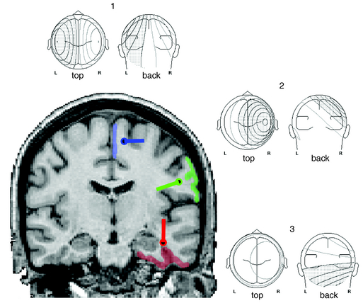
With renewed appreciation for the biophysics of EEG generation, we now realize that this assumption is true only in limited cases in which the spike or seizure voltage field is purely radial in its orientation.¹ Such fields are typically generated by the crowns of convexity cortex. However, many brain regions that are highly epileptogenic are not found on the cortical convexity. This includes the entire base of the brain, in particular orbitofrontal and basal temporal regions. These cortices produce EEG fields that are tangential to the head surface rather than radial. Similarly, epileptogenic foci in major fissures, such as Sylvian or interhemispheric, produce tangentially oriented EEG fields. Such sources are important to understand because little or no EEG potential is recorded directly above them; rather, the negative and positive EEG fields on the head are displaced on either side of their true location. In such a situation, considering the negative field maximum as the source location will result in false localization and even a false lateralization in certain situations (Figure 5-1).

Figure 5–1 Three cortical sources are noted by color overlay on the MRI—interhemispheric (blue), lateral convexity (green), and temporal base (red). Scalp voltage fields produced by depolarization of these sources (1, 2, and 3, respectively) are depicted surrounding the MRI. Isopotential lines denote field amplitude; speckled field is negative in polarity. An equivalent current dipole for each voltage field is shown adjacent to the cortical source. Note that the orientation of the dipole is orthogonal to the net orientation of the source cortex, and the position of the dipole is deep to the cortical surface.

EEG Fields from Cortical Sources

In the generation of any cortical EEG potential, be it epileptiform or normal, current sinks and sources are created on opposite ends of the palisaded pyramidal cells. By electromagnetic necessity, the extracellular space at one end of this cell layer is relatively negative, and the other end is relatively positive. This separation of charge creates a dipole. EEG potentials are characteristically dipolar in nature because of this generating mechanism. In epileptiform activity, the superficial laminae are often depolarized initially, leading to the prominence of negative potentials for epileptic spikes and seizure potentials. Of note, this is the opposite of normal sensory-evoked potentials, where depolarization of layer 4 results in passive hyperpolarization of the superficial laminae and a resultant surface-positive potential. Recurrent circuits within the cortex produce reverberating depolarization/hyperpolarization sequences. Thus many cortical potentials, including epileptic activity, exhibit recurrent cycling of negative and positive waveforms, such as in spike-wave complexes. All cortical EEG potentials have a dipolar field configuration; however, given limited spatial sampling of scalp electrodes, we may not record both sides of this dipole field. This is particularly true for radial sources near the vertex that have a positive field maximum at the bottom of the head. Conversely, for basal brain sources only the positive field maximum may be recordable from standard 10 to 20 electrode positions. However, for sources in the lateral aspect of the brain, both maxima are typically evident in traditional montages (see Figure 5-1).

A three-dimensional line drawn between the negative and positive field maximum of a spike potential on the head has the same orientation as that of the pyramidal cells generating the potential. The actual cortical source may be geometrically complex, but this line represents the net orientation of those cells. Because pyramidal cells are orthogonal to the cortical surface, the orientation of an EEG field is also orthogonal to the source cortex. Theoretically, the center of the cortical source must lie along this 3-D line. Its location is proportionally nearer the field maximum with greater amplitude. Thus, in most cases sources are located nearer the higher amplitude negative field maximum. However, when the voltage field is tangential, the source location is equidistant between field maxima. Simply by inspecting the spike/seizure voltage fields over the head, one can gain considerable information about the likely source of these fields. Such visual analysis is essentially a form of source modeling. This same spatial information regarding voltage fields is the basic data used by all source modeling mathematical algorithms.

The Dipole as a Model of Cortical Sources

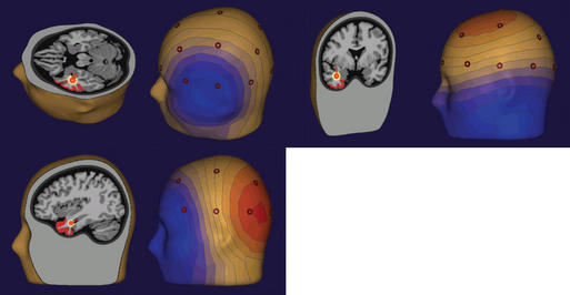
The most common source modeling technique used for clinical applications is the single equivalent current dipole.² As noted earlier, cortical sources of EEG spikes or seizure rhythms produce voltage fields that are dipolar in nature. It makes sense, therefore, to use a model that is dipole based. However, the dipole used in modeling is a theoretical point source with a separation of charge, whereas the actual source of an EEG potential is a relatively large region of cortex that forms a dipole layer. Although the geometry of the actual dipole layer may be complex and comprised of several gyri and sulci, the voltage fields produced by this convoluted source will add or cancel one another in a linear way to produce a resultant simple dipolar field at the scalp. In fact, recent studies of simultaneous intracranial and scalp EEG have shown that a region of gyral cortex 10 or more square centimeters in area is necessary to produce an EEG potential that is distinguishable from the ongoing background rhythm.³ In fact, large and easily identified epileptiform potentials are often generated by cortical sources of 20 to 30 cm² in size, thus encompassing a substantial sublobar region. Even though more complex multipolar geometry such as quadrapoles and octopoles may be produced by these large convoluted sources at the cortex, the dipolar field component dominates at the scalp. Because a point source dipole model attempts to explain scalp EEG fields produced by a large cortical patch, these dipole solutions are usually deep to the actual generating cortex in order to project a field of equivalent area (Figure 5-2).

Figure 5–2 Major cortical sources and their equivalent dipoles for temporal lobe spikes/seizures are illustrated—lateral cortex (top left), tip cortex (bottom left), and base cortex (top right). To the right of each source is the scalp voltage field produced by the source. Note that a three-dimensional line connecting the negative (blue) and positive (red) field maximum defines the orientation of the field and that of the equivalent dipole. Lateral temporal cortex dipoles are horizontal and radial; temporal tip dipoles are horizontal and tangential; temporal base dipoles are vertical and tangential. Note, too, that dipoles are deep to the cortical sources.

Physical laws of electromagnetic field theory state that the voltage fields on the surface of a spherical volume conductor can be accurately predicted if the location, orientation, and strength of a dipole source within the conductor are known.^4,⁵ This is called the forward solution, and it is unique. However, what we attempt to do in clinical dipole modeling is the reverse. We measure the surface voltage field on the head and attempt to identify the source within this volume conductor. This is the “inverse solution,” and it is not unique because a number of different dipolar source configurations within the brain can produce the same surface field.⁶^–⁸ Therefore, we have to use certain assumptions to minimize the possibilities, and the principal one is that the source is a single current dipole. Various algorithms exist for identifying an equivalent dipole source.⁸^–¹¹ Most of these algorithms use an iterative-minimizing approach, whereby an estimate of source location is made. The forward solution is performed, and the difference between the forward solution and the actual measured field is characterized. Subsequent random movements of the dipole model attempt to minimize this difference. When the smallest difference is obtained, the putative dipolar source has been identified.

Dipole models display in three-dimensional terms the same information that a person can perceive by visually inspecting the voltage fields as explained earlier. In addition, these equivalent dipoles can be coregistered either with a head schematic or with an actual three-dimensional magnetic resonance imaging (MRI) to identify the putative source within the brain. With a head or brain schematic, it is possible to identify the most likely lobe or perhaps even sublobar area containing the source. It is very tempting to coregister these data with three-dimensional MRIs, as is commonly done with other functional imaging techniques. The problem with doing so is that sources or colored blobs that are placed on a real brain image take on a seductive pseudorealism that in reality must be verified. In the case of EEG dipole models, sources in the cortical convexity are accurately localized. This is because even simple spherical head models used by source-modeling algorithms work well in this most spherical part of the head and brain. However, when sources were near the base of the brain, such as in the temporal lobe, systematic dipole location errors occurred for known sources.^12,¹³ This error was typically in the vertical direction toward the vertex, and it could be as great as 2 or more centimeters in magnitude. A spherical head model was the reason for this error.¹³^–¹⁵ Such a model cannot be used to localize sources near nonspherical parts of the head, such as the base of the skull (Figure 5-3).

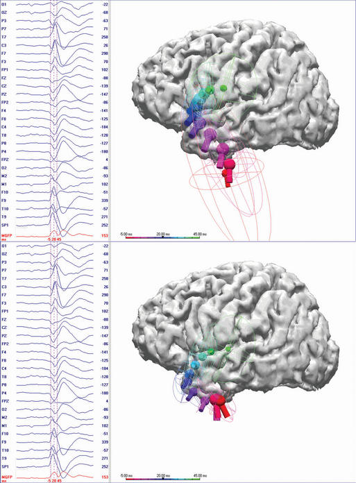
Figure 5–3 Fifty milliseconds of the same left temporal spike are depicted in moving dipole models at the top and bottom of the figure. A single dipole has been calculated for each of 11 sequential voltage field measurements at 5 msec intervals (red to green). Dipoles illustrated on the upper brain were calculated using a three-concentric-sphere head model. Dipoles on the lower brain were derived using a realistic head model. Note that both initial and late dipoles from the spherical head model are erroneously located outside the temporal lobe, whereas dipoles from the realistic head model remain in the temporal lobe.

Those surfaces that are important for the degradation of scalp EEG signals, namely the inner and outer layers of the skull and outer layer of the scalp, can be segmented with modern volumetric imaging. Using the shape of these surfaces, as determined from three-dimensional MRI and computed tomography (CT), a realistic head model can be achieved. In clinical practice, boundary element models (BEM) are most commonly used, particularly when localizing the source of potentials in nonspherical parts of the brain. The accuracy of correctly identifying temporal lobe sources, for example, is improved considerably with such models (Figure 5-3).¹⁶^–¹⁸ BEM head models can now be calculated rapidly, even on a regular PC, in a matter of minutes. Even without a patient’s individual MRI, the benefits of a realistic head model can be obtained by using one derived from standardized head images.¹⁹ Finite element head models are more complex and take into consideration differences in regional resistivity and anisotropy within the head and brain.²⁰^–²³ Accordingly, finite element models are much more difficult to compute. Regardless, it is important to use realistic head models whenever dipole models are coregistered in 3-D anatomy.

Spatial resolution of the EEG sensors influences the accuracy of source localization afforded by dipole modeling. The typical international 10-20 electrode configuration coarsely samples only the top half of the head. Recording from the “southern hemisphere” is critical for characterizing sources at the base of the brain. Twenty-six EEG channels, including a subtemporal row of three electrodes on each side of the head, is probably a minimal configuration for clinical EEG dipole modeling.² Electrode arrays that approximate the 10-10 system are better. In a study in which 128 channels of scalp EEG were progressively down-sampled to 64-, 32-, and 21-channel recordings, Lantz et al.²⁴ documented an improvement in source localization accuracy up to 64 channels. More electrodes provided little additional accuracy because the spatial frequency of dipolar scalp fields from spontaneous EEG is relatively low, and the sources of these fields are relatively large.

INTERPRETATION OF DIPOLE MODELS

It is clear from studies of simultaneous scalp and intracranial EEGs that the cortical sources of scalp spikes and seizure rhythms are quite large, namely 10 to 30 cm².³ A point source dipole is thus a simple model of this extended cortical generator, and for it to be useful, it must be interpreted properly. EEG dipoles model major cortical surfaces, not individual gyri or sulci. Dipole location identifies only the center of the source region generating the greatest potential and certainly not its extent or the specific cortex involved. Because this pointlike model tries to explain the scalp field resulting from an extended source, the model dipole is typically located deep to actual source cortex. Accordingly, one should not be concerned about dipole models in white matter. It is dipole orientation that identifies the likely source cortex within the region.²⁵^–²⁷ Dipole orientation conveys the net orientation of the pyramidal cell generating the field, and this is orthogonal to the net orientation of the generator cortex. If there is no cortex in the region of a dipole model that has an appropriate orientation, the validity of the source solution should be questioned (Figure 5-2).

Only initial epileptiform EEG activity may represent the spike source or seizure origin. Single dipole models may be misleading at the spike peak or after the early seconds of a seizure discharge. Source propagation is common, thus the temporal evolution of a dipole model is important. A dipole solution for each time point, the so-called moving dipole model, can portray propagation reasonably well if the propagation is unidirectional and until repolarization of the original source confounds the resultant voltage field (Figure 5-3). Several investigators have concluded that modeling the rising phase of the spike is more likely to represent the initial spike source²⁸^–³¹ than modeling the spike peak. Obviously there is a trade-off because the earlier time points typically have lesser signal to noise (S/N), which may make modeling less accurate. Averaging closely similar spikes or sequential ictal waveforms can improve the S/N, which will provide a more confident solution.³²

Clinical Studies Using Dipole Models

Early investigations of major clinical import were that of Ebersole and Wade.^33,³⁴ They characterized the voltage topography of spikes from a series of patients with temporal lobe epilepsy who were surgical candidates. They noted two distinctive patterns of voltage fields. One had an inferior temporal negative maximum and a vertex positive maximum, whereas the other had a lateral temporal negative maximum and a contralateral temporal positive maximum. They termed the former a Type 1 spike field and the latter a Type 2 field. Constructing a three-dimensional line between these field maxima demonstrates that the Type 2 spike has a radial field orientation, and the Type 1 has more of a tangential orientation. A variety of clinical correlations, as well as simultaneous scalp and intracranial EEG investigations, suggested that the Type 2 field topography and its corresponding horizontal radial dipole model originated from a lateral temporal cortical source, whereas Type 1 topography and its corresponding more vertical tangential dipole model was associated with basomesial temporal sources. However, the Type 1 spike field was not thought to reflect hippocampal or amygdalar activity directly. It was shown that spikes confined to these structures did not generate scalp-recordable voltage fields due to the small source area and curved source shape, which favor voltage cancellation.³⁵ Rather, it was the common and preferred propagation of this epileptiform activity from mesial structures into the entorhinal, fusiform, and temporal basal cortex that resulted in a generator of sufficient area to produce scalp EEG potentials.^28,^35,³⁶

Subsequent investigation demonstrated that a rigid categorization of temporal spike topography was overly simplistic. Spike voltage fields commonly evolve over tens of milliseconds, which usually signifies a propagating spike source. A Type 1 pattern may evolve into a Type 2 pattern and vice versa. Spikes that originate in basal temporal cortex frequently propagate into temporal tip cortex by the time sufficient cortex is activated to produce a scalp EEG field. Temporal tip cortex has a net anterior-facing orientation. Accordingly, spike sources in this cortex produce a scalp voltage field with a frontotemporal to frontopolar negative maximum and a posterior positive maximum ^27,^29,³⁰ (Figure 5-2). Other investigators confirmed and validated these results in additional patient populations. Most came to the same conclusion—that dipole orientation was essential for proper interpretation of source solutions.³⁷^–⁴⁰

In a series of studies, Boon et al.⁴¹^–⁴³ demonstrated that dipole orientation could differentiate patients with the basomesial temporal lobe epilepsy from those with lateral neocortical temporal lobe epilepsy. This distinction was based on dipole orientation and could be made by analyzing either spike discharges or seizure rhythms. Dipoles with a radial and horizontal orientation reflected spike or seizure activity from the lateral temporal cortices, whereas dipole models with a more vertical orientation reflected activity in the base of the temporal lobe that originated from more mesial structures. Using these criteria, Boon et al. were able to predict surgical outcomes and intracranial EEG findings. A later study by this same group showed that dipole analysis of ictal rhythms identified incongruence between a structural abnormality and the source of epileptiform EEG activity. This information could be useful in deciding not to proceed with invasive studies or surgical resection.⁴⁴ Numerous other publications appeared in the late 1990s that demonstrated that the localization provided by spike dipole modeling correlated well with other localization tools such as intracranial EEG,^45,⁴⁶ positron emission tomography,⁴⁷ single photon emission tomography,^47,⁴⁸ and MRI lesions in both adults and pediatric patients.⁴⁹

Assaf and Ebersole ⁵⁰ examined ictal recordings from the scalp EEGs of 40 patients with temporal lobe epilepsy who required invasive monitoring as part of a presurgical evaluation. The earliest recognizable seizure rhythms for each patient were averaged and analyzed using a source montage based on a fixed set of dipoles modeling defined cortical areas of the temporal lobe. Results were compared to ictal localization from intracranial recordings. A high positive predictive value was seen between vertical tangential dipoles and seizure onset in the hippocampus, between horizontal tangential dipoles and seizure onset in the temporal tip or entorhinal cortex, and finally between horizontal radial dipoles and seizure onset lateral temporal neocortex. These results from ictal data are thus comparable to findings from previous interictal studies. In a later publication, these authors⁵¹ demonstrated that the same type of dipole analysis could be used to predict surgical success. They found that those patients with a temporal ictal rhythm having a dominant and leading basal source were more likely to maintain seizure freedom following surgery than those with a lateral source.

Michel et al.⁵² recently performed the largest prospective study of interictal source modeling to date. In a group of 40 candidates for epilepsy surgery, they analyzed epileptiform EEG spikes using a distributed, rather than dipole, model. In a subgroup of 24 patients (17 with temporal and 7 with extratemporal foci) who underwent the surgery, source models of their spikes fell within the borders of the nearest surgical resection in 18 patients. Sixteen of these 18 had a class 1 Engel outcome. They also noted that the localization by source models agreed with the intracranial EEG in the seven patients who had invasive studies. The same group recently examined and demonstrated the usefulness of EEG source modeling in a presurgical cohort of pediatric epilepsy patients.⁵³