Historical overview and types of topographers

The corneal first surface is the part with the highest dioptric power of the eye. The simplest device to measure corneal curvature is the manual keratometer. It measures the distance between the first Purkinje images of two test marks along two orthogonal meridians. The distance measured is a function of corneal curvature and usually is converted into a dioptric power value by multiplying the inverse of curvature (radius) with the corneal refractive index. Corneal astigmatism is determined by measurement of two orthogonal meridians. In contrast, keratoscopy visualizes the corneal curvature and irregularities across the entire cornea: the mirrored image of a disk with concentric rings (Placido disk) on the cornea is inspected. The advent of personal computers, video cameras, and image analysis software allowed a combination of both techniques: a digital still image of the reflection on the cornea is captured and a software program calculates corneal curvature at each corneal point based on the distance of the mires in the corneal reflection image6,8. Computerized videokeratoskopy, as the novel technique was called, enabled measurement of corneal curvature across the entire cornea. In analogy to keratometry, curvature is still converted into power values and expressed as ‘keratometric diopters’. On a color contour map, curvature is plotted as a function of location, hence the more common term ‘corneal topography’.

Placido-based corneal topographers are the topographers first constructed and still most widely used. Placido topographers measure with good reliability at a high dynamic range8. One disadvantage is the sparing of the corneal center because of the location of the camera front lens. Scheimpflug photography produces optical sections of the cornea with anterior and posterior surface in focus, enabling the measurement of both anterior and posterior corneal surfaces. From raw images, corneal height, curvature and refractive power as well topographic maps of corneal thickness can be calculated. Some manufacturers (Bausch & Lomb, Ziemer) have equipped their Scheimpflug topographers with a Placido disk for anterior surface imaging, while others (Oculus, iVis) rely on the improved resolution of new generation CCD cameras and offer a Scheimpflug-only solution. Apart from corneal back surface imaging, rotating Scheimpflug cameras have the advantage of high density imaging of the central cornea, because this region is imaged in each frame. Other techniques not or not yet commercially available include raster stereography, interference fringe polarimetry, and Hartmann–Shack-based topography (iZone, Abbott Medical Optics)8.

Different types of topographic display (topographic maps)

Color-coded contour maps translate the qualitative information (raw data) into qualitative information that can be read intuitively. The maps generated from each parameter (e.g. curvature, height, refractive power) have specific characteristics that are mandatory to understand for correct interpretation. Typically, the colors chosen represent a continuous spectrum from ‘cold’ (blue) to ‘hot’ (red). The upper and lower limits of the color scale, the scale steps, and the number of colors influence the appearance of the map. Using standardized settings not only allows the comparison of exams taken from different patients or from the same patient taken at different time points, it also helps in learning to interpret corneal topographic maps.

Curvature maps plot corneal curvature as a function of location on the cornea and are the maps most commonly used in ophthalmological practice. The convention of representing curvature in diopters rather than in millimeters is based on historical reasons and has its origins in manual keratometry. Therefore, it is important to stress that curvature maps do not represent corneal refractive power, because refractive power is proportional to the curvature only in a paraxial 2 mm region of the cornea. There are two common ways to calculate and display corneal curvature: axial and meridional (tangential or instantaneous) maps. Reconstruction of the non-uniform curvature along each meridian is achieved by fitting a circle to a region of interest. The radius of curvature (ROC) of the best-fit circle equals the corneal ROC in that certain region of interest. On an axial curvature map the center of the circle is located on the sagittal axis (hence the term axial), while on meridional (tangential or instantaneous) maps the center of the circle is variable and circles are fitted along a corneal meridian (hence the term meridional). These two methods of calculation create the characteristic difference in the appearance of the two map types: axial maps have a smoother appearance biased towards a more spherical shape of the cornea (Fig. 22.1). Conversely, meridional maps show a greater variance of curvature along the meridians and therefore are suited well for revealing local irregularities of the cornea, especially those in more peripheral corneal regions (see Fig. 22.1).

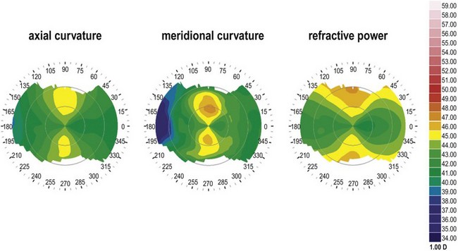
Fig. 22.1 Corneal curvature maps. All three maps are based on the same raw data and the same color scale.

Refractive power maps display corneal refractive power and can be calculated by applying Snell’s law or ray trace calculations that take spherical aberration from the paraxial cornea and effects of the posterior corneal surface into account (see Fig. 22.1).

Elevation maps became popular with the advent of Scheimpflug topography. Like on a topographic map of the Earth where height is displayed as difference from the sea level, on a corneal elevation map height is displayed as the difference from a predefined reference plane (Fig. 22.2, top). In most cases a sphere (the best-fit sphere, BFS) is used as a reference plane, because a plain reference plane would not reveal local irregularities of shape due to the spherical shape of the cornea (see Fig. 22.2, top). Typically, the BFS is fitted to the raw data by varying its ROC and its position relative to the viewing axis in order to minimize the root-mean square difference between measured data and the BFS (float mode). Other calculation modes (axis, pinned, apex) apply certain constraints to the position of the BFS and emphasize different characteristics of corneal shape. In analogy to geographic maps, elevations above the BFS (‘mountains’) are coded with warm colors, points on the BFS are coded green (‘land’) and points below the BFS are coded with cold colors (’sea’). This allows an intuitive assessment of the corneal shapes, particularly of deviations from spherical shape.

Fig. 22.2 Corneal elevation and wavefront error maps. All maps are based on the same raw data. The top row shows the different appearance of elevation maps if different reference planes (sphere vs. plane) are used. The bottom row shows corneal first-surface wavefront error maps (6 mm analysis pupil diameter) of the same eye.

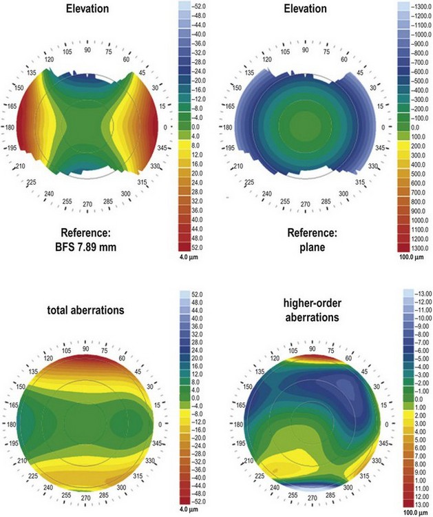
From the raw data of each map, metrics for quantification can be calculated. The metrics offered by the software vary from device to device, because often proprietary algorithms are used, e.g. for keratoconus detection. Based on curvature data, simulated keratometry (sim K) values simulate the readings of a manual keratometer while irregularity indices reflect the variance of curvature in a defined region of interest. Other curvature metrics include the location of the apex and a variety of indices for keratoconus detection5,9. From elevation maps, distances from the BFS (clinically often referred to as ‘elevation’) in a single point or within a defined region of interest can be calculated. The ROC of the BFS roughly reflects the corneal ROC. All elevation metrics are highly dependent on the shape of the reference plane (e.g. BFS), the region the BFS was fitted over, and the mode of fit (e.g. float). Another useful method for quantification of corneal topography measurements is to perform a Zernike or Fourier decomposition of the corneal anterior or posterior surface data (Fig. 22.2, bottom)7. Based on the input data, either shape (elevation, curvature) or optical properties (ray-trace from refractive power data) of the corneal surfaces can be determined. This analysis is particularly useful for outcome analysis in corneal refractive surgery or keratoconus detection1,3.

Use of corneal topography in refractive surgery

In refractive surgery, corneal topography is essential both for preoperative assessment and for postoperative follow-up. Preoperatively, screening for conditions that are contraindications for corneal procedures (e.g. keratoconus, pellucid marginal degeneration, PMD) or bear the risk of complications (e.g. excessively flat or steep radii of curvature) is imperative. Astigmatism could easily be recognized by its characteristic bow-tie pattern on the map where the ‘hot’ colors represent the steep axis (see Fig. 22.1). A hallmark of corneal ectatic diseases like keratoconus and PMD is an asymmetric bow-tie with skewed radial axes or a localized inferior steepening. A variety of metrics calculated from the topographic data can help with the decision if an eye is suspicious for keratoconus or PMD1,5,9. Another important preoperative application is treatment planning for astigmatic corrections (limbal relaxing incisions, astigmatic keratotomy, intracorneal ring segments, and toric intraocular lenses). Often, corneal shape data are required besides ocular wavefront data for customized corneal ablation.

Postoperatively, corneal topography is an important tool for outcome assessment because it provides information about the optical quality of the cornea that can be correlated with clinical outcome. Corneal topography reveals whether ecximer ablations are centered correctly and astigmatism is fully corrected. Moreover, surface irregularity due to post-LASIK dry eye syndrome or to epithelial healing problems after surface ablation (PRK, LASEK, epiLASIK) can be classified. For long-term follow-up, corneal topography is necessary to detect iatrogenic ectasia and regression in coagulative procedures like cK or LTK.

Historical overview and types of wavefront sensors

The influence of optical media on propagation of light waves is reflected by the wavefront. The wavefront is a plane connecting light waves in a point of equal phase. It is perpendicular to the light ray and therefore mirrors the optical properties of a certain optical system. Every deviation of an optical system from being an ideal diffraction-limited system is represented by the deviation of the actual wavefront compared with an ideal wavefront. Bille and coworkers were the first to measure the ocular wavefront aberration in 1978. Since then, wavefront sensing (aberrometry) emerged from a lab application to a universal ophthalmological tool4. The ocular wave deformation comprehensively reflects the optical properties of the eye. This is important clinically, because with conventional techniques only spherical and cylindrical error (so-called lower order aberrations) can be measured. However there are optical aberrations (so-called higher order aberrations) that could neither be measured with conventional techniques nor be corrected with spectacles. These aberrations (e.g. spherical aberration and coma) have been known for a long time because of their characteristic image degrading patterns but only wavefront sensing techniques allowed their quantification.

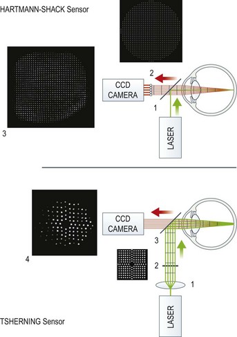
The most common wavefront sensor is the Hartmann–Shack aberrometer (Fig. 22.3, top). In this, a laser beam is projected onto the retina and the light emerging from the eye is led via a beam splitter [1] though a microlens array [2] and the spot pattern [3] created by the microlenses is captured by a CCD camera. In the case of ideal, diffraction-limited optics (no aberrations) the spots have equal distances like the lens array. Any deviation from this ideal pattern is proportional to deviations in the wavefront allowing calculation of the wave aberrations. The Tscherning aberrometer (see Fig. 22.3, bottom) also uses spot matrix analysis. A collimated laser beam [1] is sent through an array of spots [2] and projected onto the retina [4]. Deviations from the ideal position reflect aberrations of the wavefront. Ray tracing aberrometers (commercially available as iTrace, Tracey Technologies) use the same technique; however, the projection of spots is done sequentially. This avoids confusion due to spot overlap in highly distorted wavefronts and enhances the dynamic range of the wavefront sensor. Dynamic skiascopy (spatially resolved refractometry) measures wavefront errors by locally determining refractive power within the pupil. In contrast to corneal topography, aberrometric measurements require clear optical media to obtain valid results. Furthermore, the region of interest is limited by the pupil diameter, which often makes pupil dilation, either physiological or pharmacological, necessary.

Fig. 22.3 Functional principles of wavefront sensors. Top, Hartmann–Shack sensor: [1] beam splitter; [2] microlens array; [3] spot pattern image. Bottom, Tscherning sensor: [1] collimator; [2] aperture with spot pattern; [3] beam splitter; [4] spot pattern image. Green: light from laser to retina; red: light emerging from the eye.

Wavefront reconstruction and analysis

From the raw data captured by the wavefront sensor, the slope of the wavefront at each point of interest (i.e. each spot of the point matrix) can be calculated. While from these data a coarse color map plotting the wavefront deviation as a function of pupil location can be constructed, only the technique known as Zernike decomposition allows quantification of wavefront aberrations10. A set of orthogonal mathematical functions over the unit circle, Zernike polynomials, are fitted to the raw data by creating a sum function (the wavefront function). Each polynomial represents a specific shape; many of the shapes are analogous to wavefront deformations caused by certain aberrations (e.g. spherical defocus, astigmatism, coma, spherical aberration). By this method, two important goals are achieved: first, the space between the data points is interpolated, second and more important, the presence of each polynomial within the wavefront function reflects a characteristic shape of the wavefront. Each polynomial is reflected by a coefficient, indicating the dominance of a certain polynomial in the wavefront function. The entire set of these Zernike coefficients can be used to reproducibly and unambiguously quantify almost any irregular wavefront shape. The formulas of Zernike polynomials follow systematic rules describing the radial and azimuthal spatial variation, which are described by the radial order of the polynomial and by the meridional frequency respectively. The more polynomials are used for reconstruction, the higher the order required and the less the residual fit error. Applying Fourier transformation, from Zernike coefficients the point spread function (PSF) and the modulation transfer function (MTF), which both reflect retinal image quality, can be calculated. For clinical use, comprehensive metrics like the root mean square (RMS) of the wavefront error, of lower and higher orders, and of homologous aberrations are used frequently. Complex optical quality metrics based on PSF and MTF such as the visual Strehl ratio based on the optical transfer function (VSOTF) reflect both qualitative and quantitative aspects2.

Use of wavefront sensing in refractive surgery

For the majority of refractive surgeons, wavefront sensors generate the input data for wavefront-guided excimer procedures. Thus, an aberrometer is almost always integral part of a commercially available laser platform. Like in all biometric measurements there can be a high intra-patient variability due to microfluctuations of accommodation and tear film break-up. For this reason, most aberrometers capture and average several repeated measurements automatically, especially if data are used for wavefront-guided excimer procedures. Combined topography/aberrometer units which capture corneal and ocular wavefront without need for realigning the instrument allow location of the source of certain aberrations (corneal vs. lenticular). This can be extremely helpful for finding the optimum treatment in cases of early cataract. For postoperative follow-up of corneal refractive procedures, corneal topography might be sufficient in the majority of cases. However, one should be aware that comprehensive evaluation of the optical properties of the eye can be achieved only in combination with aberrometry.