Chapter 3 Clinical Pharmacokinetics and Issues in Therapeutics
| Abbreviations | |
|---|---|
| AUC | Area under the drug plasma concentration–time curve |
| Css | Steady-state concentration of drug |
| C(t) | Concentration of drug in plasma at any time “t” |
| CL | Clearance |
| CLp | Plasma clearance |
| E | Hepatic extraction ratio |
| F | Bioavailability |
| GI | Gastrointestinal |
| IA | Intraarterial |
| IM | Intramuscular |
| IV | Intravenous |
| Q | Hepatic blood flow |
| SC | Subcutaneous |
| t1/2 | Half-life |
| T | Dosing interval |
| TI | Therapeutic index |
| Vd | Apparent volume of distribution |
When planning drug therapy for a patient, deciding on the choice of drug and its dosing schedule is obviously critical. To make such decisions, an observable pharmacological effect is usually selected, and the dosing rate is manipulated until this effect is observed. This approach works quite well with some drugs. For example, blood pressure can be monitored in a hypertensive patient (Fig. 3-1, Drug A) and the dose of drug modified until blood pressure is reduced to the desired level. However, for other drugs this approach is more problematic, usually because of the lack of an easily observable effect, a narrow TI (ratio of therapeutic to toxic dose), or changes in the condition of the patient that require modification of dosing rate.
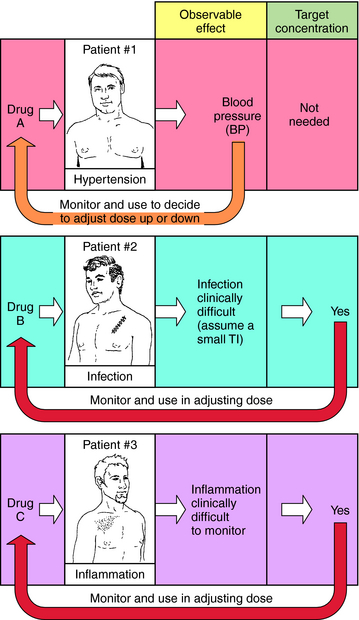
For example, when an antibiotic with a low TI is used to treat a severe infection (Fig. 3-1, Drug B), it can be difficult to quantify therapeutic progress, because a visible effect is not apparent immediately. Because of its narrow TI, care must be taken to ensure that the drug concentration does not become too high and cause toxicity. Similarly, if the desired effect is not easily visualized because of other considerations, such as inflammation in an internal organ, this approach is also problematic (Fig. 3-1, Drug C). Finally, changes in the condition of the patient can also necessitate adjustments in dose rates. For example, if a drug is eliminated through the kidneys, changes in renal function will be important. Without an observable effect that is easily monitored (as with drugs B and C), it is not always clear that such adjustments are beneficial.
schedule, and the mode and route of administration must be specified. Pharmacokinetic considerations have a major role in establishing the dosing schedule, or in adjusting an existing schedule, to increase effectiveness of the drug or to reduce symptoms of toxicity.
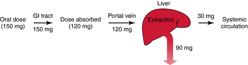
Major routes of administration are divided into (1) enteral, drugs entering the body via the gastrointestinal (GI) tract, and (2) parenteral, drugs entering the body by injection. Specific examples are given in Box 3-1. The oral route is most popular because it is most convenient. However, poor absorption in the GI tract, first-pass metabolism in the liver, delays in stomach emptying, degradation by stomach acidity, or complexation with food may preclude oral administration. Intramuscular (IM), subcutaneous (SC), and topical routes bypass these problems. In many cases absorption into the blood is rapid for drugs given IM and only slightly slower after SC administration. The advantage of the intravenous (IV) route is a very rapid onset of action and a controlled rate of administration; however, this is countered by the disadvantages of possible infection, coagulation problems, and a greater incidence of allergic reactions. Also, most injected drugs, especially when given IV, require trained personnel.
Single-Dose IV Injection and Plasma Concentration
If a drug is injected into a vein as a single bolus over 5 to 30 seconds and blood samples are taken periodically and analyzed for the drug, the results appear as in Figure 3-2, A. The concentration will be greatest shortly after injection, when distribution of drug in the circulatory system has reached equilibrium. This initial mixing of drug and blood (red blood cells and plasma) is essentially complete after several passes through the heart. Drug leaves the plasma by several processes:
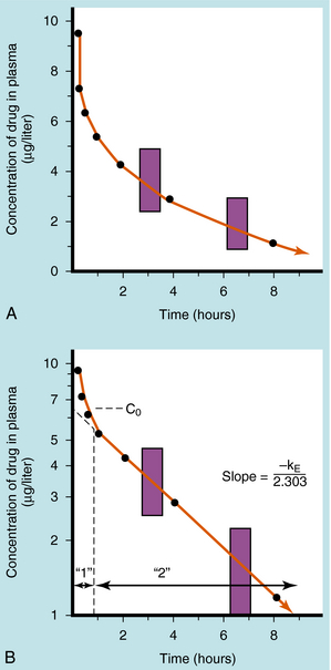
Some of the drug in plasma is bound to proteins or other plasma constituents; this binding occurs very rapidly and usually renders the bound portion of the drug inactive. Similarly, a considerable fraction of the injected dose may pass through capillary walls and bind to extravascular tissue, also rendering this fraction of drug inactive. The values of drug concentration plotted on the vertical scale in Figure 3-2 represent the sum of unbound drug and bound drug. Note that the concentration-time profile shows continuous curvature.
If concentrations are plotted on a logarithmic scale (Fig. 3-2, B), the terminal data points (after 1 hour) lie on a straight line. The section marked “1” on this graph represents the distribution phase (sometimes called alpha phase), representing the main process of drug distribution across membranes and into body regions that are not well perfused. Section “2” (beta phase or elimination) represents elimination of the drug, which gradually decreases plasma concentration. In many clinical situations, the duration of the distribution phase is very short compared with that of the elimination phase.
If the distribution phase in Figure 3-2 (A or B) is neglected, the equation of the line is:

where:
Equation 3-1 describes a curve on an arithmetic scale (Fig. 3-2, A) that becomes a straight line on a semilogarithmic scale (Fig. 3-2, B). In this case the slope will be –kE/2.3, and the y-intercept is log C0. A characteristic of this type of curve is that a constant fraction of drug dose remaining in the body is eliminated per unit time.
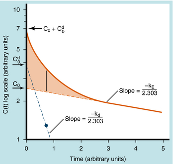
When elimination is rapid, the error in describing C(t) becomes appreciable if the distribution phase is omitted. Although the mathematical derivation is beyond the scope of this text, such a situation is plotted in Figure 3-3 to emphasize the importance of the distribution phase. For most drugs, distribution occurs much more rapidly than elimination, and therefore the distribution term becomes zero after only a small portion of the dose is eliminated. By back extrapolation of the linear postdistribution data, the value of C0 can be obtained, whereas kE can be determined from the slope. The concentration component responsible for the distribution phase (shaded area in Fig. 3-3) is obtained as the difference between the actual concentration and the extrapolated elimination line. This difference can be used to calculate the rate constant for distribution (kd) and the extrapolated time zero-concentration component for the distribution phase  . However, this complexity is often ignored because C(t) for many drugs can be described adequately in terms of the monoexponential equation 3-1. Therefore this chapter discusses only the postdistribution phase kinetics described by equation 3-1.
Single Oral Dose and Plasma Concentration
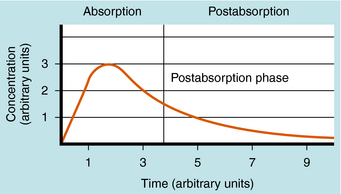
The plot of C(t) versus time after oral administration is different from that after IV injection only during the drug absorption phase, assuming equal bioavailability. The two plots become identical for the postabsorption or elimination phase. A typical plot of plasma concentration versus time after oral administration is shown in Figure 3-4. Initially, there is no drug in the plasma because the preparation must be swallowed, undergo dissolution if administered as a tablet, await stomach emptying, and be absorbed, mainly in the small intestine. As the plasma concentration of drug increases as a result of rapid absorption, the rate of elimination also increases, because elimination is usually a first-order process, where rate increases with increasing drug concentration. The peak concentration is reached when the rates of absorption and elimination are equal.
CALCULATION OF PHARMACOKINETIC PARAMETERS
As shown in Figures 3-2 and 3-4, the concentration-time profile of a drug in plasma is different after IV and oral administration. The shape of the area under the concentration-time curve (AUC) is determined by several factors, including dose magnitude, route of administration, elimination capacity, and single or multiple dosing. In experiments the information derived from such profiles allows derivation of the important pharmacokinetic parameters—clearance, volume of distribution, bioavailability, and t 1/2. These terms are used to calculate drug dosing regimens.
Drug clearance is defined as the volume of blood cleared of drug per unit time (e.g., mL/min) and describes the efficiency of elimination of a drug from the body. Clearance is an independent pharmacokinetic parameter; it does not depend on the volume of distribution, t1/2, or bioavailability, and is the most important pharmacokinetic parameter to know about any drug. It can be considered to be the volume of blood from which all drug molecules must be removed each minute to achieve such a rate of removal (Fig. 3-5). Chapter 2 contains descriptions of the mechanisms of clearance by renal, hepatic, and other organs. Total body clearance is the sum of all of these and is constant for a particular drug in a specific patient, assuming no change in patient status.
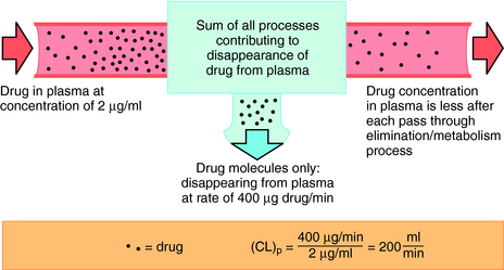
The plot of C(t) versus time (see Fig. 3-2) shows the concentration of drug decreasing with time. The corresponding elimination rate (e.g., mg/min) represents the quantity of drug being removed. The rate of removal is assumed to follow first-order kinetics, and total body clearance can be defined as follows:
where CLp indicates total body removal from plasma (p).


| Body Weight | Body H2O (percentage) | Volume (approx. liters) |
|---|---|---|
| Plasma | 4 | 3 |
| Extracellular | 20 | 15 |
| Total body | 60 | 45 |
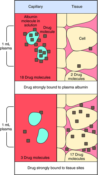
Experimental values of Vd vary from 5 to 10 L for drugs, such as warfarin and furosemide, to 15,000 to 40,000 L for chloroquine and loratadine in a 70 kg adult. How can one have Vd values grossly in excess of the total body volume? This usually occurs as a result of different degrees of protein and tissue binding of drugs and using plasma as the sole sampling source for determination of Vd (Fig. 3-6). For a drug such as warfarin, which is 99% bound to plasma albumin at therapeutic concentrations, nearly all the initial dose is in the plasma; a plot of log C(t) versus time, when extrapolated back to time zero, gives a large value for C0 (for bound plus unbound drug). Using a rearranged equation 3-4, Vd = D/C0, the resulting value of Vd is small (usually 2 to 10 L). At the other extreme is a drug such as chloroquine, which binds strongly to tissue sites but weakly to plasma proteins. Most of the initial dose is at tissue sites, thereby resulting in very small concentrations in plasma samples. In this case a plot of log C(t) versus time will give a small value for C0 that can result in Vd values greatly in excess of total body volume.

Equation 3-1 for C(t) was given earlier without explanation of its derivation or functional meaning. Experimental data for many drugs demonstrate that the rates of drug absorption, distribution, and elimination are generally directly proportional to concentration. Such processes follow first-order kinetics because the rate varies with the first power of the concentration. This is shown quantitatively as:

where dC(t)/dt is the rate of change of drug concentration, and kE is the elimination rate constant. It is negative because the concentration is being decreased by elimination.
Half-life (t1/2) is defined as the time it takes for the concentration of drug to decrease by half. The value of t1/2 can be read directly from a graph of log C(t) versus t, as shown in Figure 3-2. Note that t1/2 can be calculated following any route of administration (e.g., oral or SC). Values of t1/2 for the elimination phase range in practice from several minutes to days or longer for different drugs.


Binding of Drug to Plasma Constituents
The binding of drugs to plasma or serum constituents involves primarily albumin, α1-acid glycoprotein, or lipoprotein (Table 3-1). Serum albumin is the most abundant protein in human plasma. It is synthesized in the liver at roughly 140 mg/kg of body weight/day under normal conditions, but this can change dramatically in certain disease states. Many acidic drugs bind strongly to albumin, but because of the normally high concentration of plasma albumin, drug binding does not saturate all the sites. Basic drugs bind primarily to α1-acid glycoprotein, which is present in plasma at much lower concentrations than albumin but varies more widely between and within people as a result of disease. Less is known about drug binding to lipoproteins, although this is also often altered during disease.
TABLE 3–1 Drugs that Bind Appreciably to Serum or Plasma Constituents
| Bind Primarily to Albumin | Bind Primarily to α1-Acid Glycoprotein | Bind Primarily to Lipoproteins |
|---|---|---|
| Barbiturates | Alprenolol | Amphotericin B |
| Benzodiazepines | Bupivacaine | Cyclosporin |
| Bilirubin* | Dipyridamole | Tacrolimus |
| Digitoxin | Disopyramide | |
| Fatty acids* | Etidocaine | |
| Penicillins | Imipramine | |
| Phenylbutazone | Lidocaine‡ | |
| Phenytoin | Methadone | |
| Probenecid | Prazosin | |
| Streptomycin | Propranolol | |
| Sulfonamides | Quinidine | |
| Tetracycline | Sirolimus | |
| Tolbutamide | Verapamil | |
| Valproic acid | ||
| Warfarin |
Continuous Intravenous Infusion
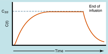
During continuous infusion the drug is administered at a fixed rate. The plasma concentration of drug gradually increases and plateaus at a concentration where the rate of infusion equals the rate of elimination. A typical plasma concentration profile is shown in Figure 3-7. The plateau is also known as the steady-state concentration (Css). Key points are:
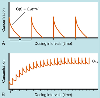
Alterations in plasma concentration of drug versus time for multiple dosing by repeated IV injections is shown in Figure 3-8. In panel A, T is selected so that all drug from the previous dose disappears before the next dose is injected and there is no accumulation of drug; no plateau or steady-state is reached. If a plateau concentration is desired, T must be short enough so that some drug from the previous dose is still present when the next dose is administered. In this way the plasma concentration gradually increases until the drug lost by elimination during T is equal to the dose of drug added at the start of T. When this is achieved, the mean concentration for each time period has reached a plateau. This stepwise accumulation is illustrated by panel B in Figure 3-8, where a plot of plasma drug concentration versus time for multiple IV injections is shown, with T roughly equivalent to the t1/2 of drug elimination. The average rate (over a dose interval) of drug input is constant at D/T. The amount of drug eliminated is small during the first T but increases with drug concentration during subsequent intervals, until the average rate of elimination and the average rate of input are equal. That is, the dose is eliminated during T. For significant accumulation, T must be at least as short as the t1/2 and preferably shorter.

If all of the multiple doses are the same size, the term maintenance dose is used. In certain clinical situations, however, a more rapid onset of action is required, which can be achieved by giving a much larger, or loading dose, before starting the smaller maintenance dose regimen. A single IV loading dose (bolus) is often used before starting a continuous IV infusion, or a parenteral or oral loading dose may be used at the start of discrete multiple dosing. Ideally, the loading dose is calculated to raise the plasma drug concentration immediately to the plateau target concentration (see Equation 3-5), and the maintenance doses are designed to maintain the same plateau concentration. Multiplying the plateau concentration by the Vd results in a value for the loading dose (see Equation 3-5). However, the uncertainty in Vd for individual patients usually leads to administration of a more conservative loading dose to prevent overshooting the plateau and encountering toxic concentrations. This is particularly important with drugs with a narrow TI.
The once-a-day dosing interval is convenient, so you now specify 0.125 mg/day (one-half tablet/day); a 50% reduction in the plateau level requires a 50% decrease in dose. There are two options for reaching the lower plateau: (1) immediately switch to the 0.125 mg/day dosing rate and achieve the 1.6 ng/mL concentration in approximately five half-lives (you do not know what the t1/2 for digoxin is in your patient), or (2) stop the digoxin dosing for an unknown number of days until the concentration reaches 1.6 ng/mL, and then begin again at a dosing schedule of 0.125 mg/day. The second procedure undoubtedly will be more rapid, but you must determine how many days to wait. You decide to stop all digoxin dosing, wait 24 hours from the previous 3.2 ng/mL sample, and get another blood sample. The concentration now has decreased to 2.7 ng/mL or by approximately one-sixth in a day. From equation 3-1, the fractional decrease each day should remain constant. Therefore a decrease of one-sixth of the remaining concentration each day should result in 2.25 ng/mL after day 2, 1.85 ng/mL after day 3, and 1.55 ng/mL after day 4. Therefore, by withholding drug for a total of 4 days, you can reduce the plasma concentration to 1.6 ng/mL. Because the t1/2 is calculated to be 3.8 days in this patient, switching to the 0.125 mg/day dosing rate without withholding drug would have required 15 to 19 days to reach the 1.6 ng/mL concentration.
Elimination refers to the removal of drug from the body. There are two processes involved in drug elimination, as discussed in Chapter 2: metabolism, in which there is conversion of the drug to another chemical species, and excretion, in which there is loss of the chemically unchanged form of the drug. The two principal organs of elimination are the liver and kidneys. The liver is mainly concerned with metabolism but has a minor role in excretion of some drugs into the bile. The kidney is mainly involved in drug excretion.

PHYSIOLOGICAL CONCEPTS OF CLEARANCE AND BIOAVAILABILITY

Most hepatically eliminated drugs are classified as being either of low or high (hepatic) clearance. This makes it possible to predict the influence of altered liver function or drug interactions on plasma concentrations and pharmacological response. For example, metabolism of a drug is often reduced in patients with liver disease, or when a second drug inhibits its metabolic enzyme. For a high-clearance drug, this results in no change in the plasma concentration-time profile after IV dosing, because blood flow is the sole determinant of clearance (whereas plasma and tissue binding are determinants of Vd). However, when the drug is administered orally, a decrease in metabolism will result in a small reduction in E and therefore a large increase in bioavailability, resulting in substantially increased plasma concentrations. For a low hepatic clearance drug, a decrease in metabolism will cause increased concentrations after IV dosing, because metabolism is a determinant of clearance. There will be no change in bioavailability, however, because that is already close to 100%. On the other hand, concentrations after oral dosing will be raised because clearance has decreased. The outcome of this scenario is that for a low-clearance drug, both the oral and IV dose may need to be reduced to avoid toxicity, but for a high-clearance drug, only the oral dose may need adjustment (Fig. 3-9).
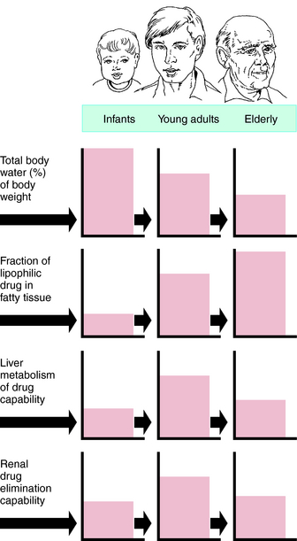
Pharmacokinetic, pharmacodynamic, and pharmacological responses differ between young adults and infants and between young adults and the elderly. These differences are due to the many physiological changes that occur during the normal life span, but especially at the extremes—infants and the elderly (Fig. 3-10).
The rational use of drugs by the elderly population (>65 years) is a challenge for both patient and prescriber. Compared with young adults, the elderly have an increased incidence of chronic illness and multiple diseases, take more drugs (prescription and over-the-counter) and drug combinations, and have more adverse drug reactions. Inadequate nutrition, decreased financial resources, and poor adherence to medication schedules may also contribute to inadequate drug therapy. These factors are compounded by the decline in physiological functions as part of the normal aging process, leading to altered drug disposition and sensitivity (Box 3-2). The elderly can have a different and more variable response to drugs compared with young adults. Drug selection and decisions about dosage in the elderly are largely based on trial and error, anecdotal data, and clinical impression. After the most appropriate drug is selected, the dosing schedule should be “start low, go slow.”
PHARMACOKINETIC CHANGES WITH AGING
Hepatic Clearance and First-Pass Metabolism
For drugs with a high hepatic clearance, the age-related decline in total liver blood flow of approximately 40% results in a similar reduction in total body clearance. The effect on first-pass hepatic extraction (and hence bioavailability) is complicated by potential alterations in other physiological variables such as protein binding and enzyme activity. In healthy elderly subjects, first-pass metabolism and bioavailability are generally not markedly altered. However, on chronic oral dosing, the higher plasma concentrations often observed in the elderly are the result of reduced phase I metabolism, irrespective of whether the drug has a high or low hepatic clearance.
DRUG RESPONSE CHANGES ASSOCIATED WITH AGING
Changes in drug responses in the elderly have been less studied than have pharmacokinetic changes. In general, an enhanced response can be expected (Table 3-2), and a reduced dosage schedule is recommended to prevent serious side effects for many drugs. Reduced responses to some drugs, such as the β-adrenergic receptor agonist isoproterenol, do occur, however, through nonpharmacokinetic mechanisms such as age-related changes in receptors and postreceptor signaling mechanisms, changes in homeostatic control, and disease-induced changes.
| Drugs | Direction of Change |
|---|---|
| Barbiturates | Increased |
| Benzodiazepines | Increased |
| Morphine | Increased |
| Pentazocine | Increased |
| Anticoagulants | Increased |
| Isoproterenol | Decreased |
| Tolbutamide | Decreased |
| Furosemide | Decreased |
Changes in Receptors and Postreceptor Mechanisms
The function of the β-adrenergic receptor system is reduced in the elderly (see Table 3-2). The sensitivity of the heart to adrenergic agonists is decreased in elderly subjects, and a higher dose of isoproterenol is required to cause a 25-beat/min increase in heart rate. However, α-adrenergic receptor function is not usually changed in the elderly.
It is common for elderly patients to have multiple chronic diseases such as diabetes, glaucoma, hypertension, coronary artery disease, and arthritis. The presence of multiple diseases leads to the use of multiple medications, an increased frequency of drug-drug interactions, and adverse drug reactions (Table 3-3). Moreover, a disease may increase the risk of adverse drug reactions or preclude the use of the otherwise most effective or safest drug for treatment of another problem. For example, anticholinergic drugs may cause urinary retention in men with enlarged prostate glands or precipitate glaucoma, and drug-induced hypotension may cause ischemic events in patients with vascular disease.
| Drug | Disease |
|---|---|
| Ibuprofen, other NSAIDs | GI tract hemorrhage, increased blood pressure, renal impairment |
| Digoxin | Dysrhythmias |
| Levothyroxine | Coronary artery disease |
| Prednisone, other glucocorticoids | Peptic ulcer disease |
| Verapamil, diltiazem | Congestive heart failure |
| Propranolol, other β-adrenergic antagonists | Congestive heart failure, chronic obstructive pulmonary disease |
NSAIDs, Nonsteroidal anti-inflammatory drugs.
Bartelink IH, Rademaker CM, Schobben AF, van den Anker JN. Guidelines on paediatric dosing on the basis of developmental physiology and pharmacokinetic considerations. Clin Pharmacokinet. 2006;45:1077-1097.
Bauer LA. Applied clinical pharmacokinetics. New York: McGraw Hill, 2001.
Birkett DJ. Pharmacokinetics made easy. Sydney: McGraw Hill, 2002.
Johnson JA. Predictability of the effects of race or ethnicity on pharmacokinetics of drugs. Int J Clin Pharmacol Ther. 2000;38:53-60.