Biomechanical Principles
NEWTON’S LAWS: UNDERLYING PRINCIPLES OF BIOMECHANICS
Newton’s Laws of Motion
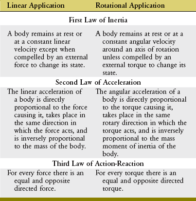
This chapter uses Newton’s laws of motion to introduce techniques for analysis of the relationship between the forces applied to the body and the consequences of those forces on human motion and posture. (Throughout the chapter, the term body is used when elaborating on the concepts related to the laws of motion and the methods of quantitative analysis. The reader should be aware that this term could also be used interchangeably with the entire human body; a segment or part of the body, such as the forearm segment; an object, such as a weight that is being lifted; or the system under consideration, such as the foot-floor interface. In most cases the simpler term, body, is used when describing the main concepts.) Newton’s laws are described for both linear and rotational (angular) motion (Table 4-1).
NEWTON’S FIRST LAW: LAW OF INERTIA
In addition to the human body as a whole, each segment, such as the arm or trunk, also has a defined center of mass. In the lower extremity, for example, the major segments include the thigh, shank (lower leg), and foot. Figure 4-1 shows the center of mass of these segments for the lower extremities of a sprinter, indicated by black circles. The location of the center of mass within each segment remains fixed, approximately at its midpoint. In contrast, however, the location of the center of mass of the entire lower extremity changes with a change in spatial configuration of the segments (compare red circles in Figure 4-1). As shown for the left (flexed) lower extremity, the specific configuration of the segments can displace the center of mass of the lower limb outside the body. Additional information regarding the center of mass of body segments is discussed later in this chapter under the topic of anthropometry.
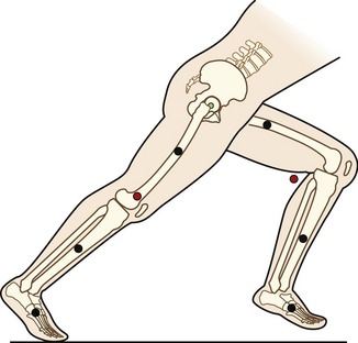
The mass moment of inertia of a body is a quantity that indicates its resistance to a change in angular velocity. Unlike inertia, its linear counterpart, the mass moment of inertia depends not only on the mass of the body, but, perhaps more important, on the distribution of its mass with respect to an axis of rotation.7 (Mass moment of inertia is often indicated by I and is expressed in units of kilograms-meters squared [kg-m2]). Because most human motion is angular rather than linear, the concept of mass moment of inertia is very relevant and important. Consider again the two positions of the lower extremities of the sprinter in Figure 4-1. Within each segment, the individual centers of mass of the thigh, shank, and foot are in the same location in both lower extremities; however, because of the different degrees of knee flexion, the distances of the centers of mass of the shank and foot segments have changed relative to the hip joint. As a consequence the mass moment of inertia of each entire limb changes; the right extended (and “longer”) lower extremity has a greater mass moment of inertia than the left. (Another way of conceptualizing the increase is to note that as the knee extends, the center of mass of the entire right lower extremity, depicted by the red circle, moves farther from the hip, thereby increasing its mass moment of inertia.) The ability to actively change an entire limb’s mass moment of inertia can profoundly affect the muscle forces and joint torques necessary for movement. For example, during the swing phase of running, the entire lower limb functionally shortens by the combined movements of knee flexion and ankle dorsiflexion (as in the left lower extremity in Figure 4-1). The lower limb’s reduced mass moment of inertia reduces the torque required by the hip muscles to accelerate and decelerate the limb during swing phase. This concept can be readily appreciated during the swing phase while running with the knees held nearly extended (increased I), or almost fully flexed (decreased I).
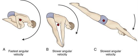
Athletes often attempt to control the mass moment of inertia of their entire body by altering the position of their individual body segments relative to the axis of rotation. This concept is well illustrated by divers who reduce their moment of inertia in order to successfully complete multiple somersaults while in the air (Figure 4-2, A). The athlete can assume an extreme “tuck” position by placing the head near the knees, holding the arms and legs tightly together, thereby bringing their segments’ centers of gravity closer to the axis of rotation. Based on the principle of “conservation of angular momentum,” reducing the body’s mass moment of inertia results in an increased angular velocity. Conversely, the athlete could slow the rotation by assuming a “pike” (see Figure 4-2, B) position and increasing the body’s moment of inertia, or assuming a “layout” position (see Figure 4-2, C), which maximizes the body’s mass moment of inertia and greatly slows the body’s angular velocity.
SPECIAL FOCUS 4-1  A Closer Mathematic Look at the Concept of Mass Moment of Inertia

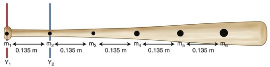
As a way to further explore Equation 4.2, it will be used to determine how the grip applied to a baseball bat dramatically affects its mass moment of inertia and therefore the difficulty in swinging the bat. The bat illustrated in Figure 4-3 is considered to consist of six point masses (m1 to m6), ranging from 0.1 to 0.225 kg, each located 0.135 m from another. During the swing the batter rotates the bat; for illustration purposes the axis of this rotation is positioned as Y1 (red line). If the bat is not sized correctly for the batter, the batter will often “choke up” by shifting his or her grip farther down the bat; again, for illustration purposes, the axis is now positioned as Y2 (blue line). The calculations shown in the box demonstrate how the distribution of the mass particles, relative to a given axis of rotation, dramatically affects the mass moment of inertia of the rotating bat. First consider Y1 as the axis of rotation. The mass moment of inertia of the bat is determined using Equation 4.2 and substituting known values. Next, consider Y2 as the axis of rotation. The important point here is that the mass particles are distributed differently when each axis is considered separately. As seen in the calculations, the mass moment of inertia when considering Y2 as the axis is 58% of that if Y1 is the considered axis. This means that the batter could achieve the same angular acceleration with 58% less torque. Or, for the same torque, the bat would accelerate 1.72 times as fast. This is a significant functional advantage gained by choking up on the bat; the bat is easier to swing, although its mass and weight have not changed. The reason for the reduced moment of inertia is that mass points m2 through m6 are closer to the Y2 axis. This is very significant mathematically when one considers that the mass moment of inertia of each point is related to the square of the distance to the axis.
The mass moment of inertia of human body segments is more difficult to determine than for the baseball bat, although they are based on the same mathematic principle. Much of the difficulty stems from the fact that segments in the human body are made up of different tissues, such as bone, muscle, fat, and skin and are not of uniform density. Values for the mass moment of inertia for each body segment have been generated from cadaver studies, mathematic modeling, and various imaging techniques.3,8
NEWTON’S SECOND LAW: LAW OF ACCELERATION
Force (Torque)-Acceleration Relationship: Newton’s second law states that the linear acceleration of a body is directly proportional to the force causing it, takes place in the same direction in which the force acts, and is inversely proportional to the mass of the body. Newton’s second law generates an equation that relates force (F), mass (m), and acceleration (a) (Equation 4.1). Conceptually, Equation 4.1 defines a force-acceleration relationship. Considered a cause-and-effect relationship, the left side of the equation, force (F), can be regarded as a cause because it represents a pull or push exerted on a body; the right side, m × a, represents the effect of the pull or push. In this equation, ΣF designates the sum of, or net, forces acting on a body. If the sum of the forces acting on a body is zero, acceleration is also zero and the body is in linear equilibrium. As previously discussed, this case is described by Newton’s first law. If, however, the net force produces acceleration, the body will accelerate in the direction of the resultant force. In this case, the body is no longer in equilibrium.

Force is measured in newtons, where 1 newton (N) = 1 kg-m/sec2.
The rotary or angular counterpart to Newton’s second law states that a torque will cause an angular acceleration of a body around an axis of rotation. Furthermore, the angular acceleration of a body is directly proportional to the torque causing it, takes place in the same rotary direction in which the torque acts, and is inversely proportional to the mass moment of inertia of the body. (The italicized words denote the essential differences between the linear and angular counterparts of this law.) For the rotary condition, Newton’s second law generates an equation that relates the torque (T), mass moment of inertia (I), and angular acceleration (α) (Equation 4.3). (This chapter uses the term torque. The reader should be aware that this term is interchangeable with terms moment and moment of force.) In this equation, ΣT designates the sum of, or net, torques acting to rotate a body. Conceptually, Equation 4.3 defines a torque–angular acceleration relationship. Within the musculoskeletal system, the primary torque producers are muscles. A contracting biceps muscle, for example, produces a net internal flexion torque at the elbow. Neglecting external influences such as gravity, the angular acceleration of the rotating forearm is proportional to the internal torque (i.e., the product of the muscle force and its internal moment arm) but is inversely proportional to the mass moment of inertia of the forearm-and-hand segment. Given a constant internal torque, the forearm-and-hand segment with the smaller mass moment of inertia will achieve a greater angular acceleration than one with a larger mass moment of inertia. (A smaller mass moment of inertia can be achieved by moving a cuff weight from the wrist to the mid-forearm, for example.) Understand that this inertial resistance to the angular acceleration of the limb applies even in the absence of gravity. For example, consider the positions of the lower limb in Figure 4-1 but with the person on his or her side in a “gravity eliminated” position. Because of changes in the mass moment of inertia, less muscular effort will be required to flex the hip with the knee also flexed than with the knee extended.

Torque is expressed in newton-meters, where 1 Nm = 1 kg-m2 × radians/sec2.
Impulse-Momentum Relationship: Additional relationships can be derived from Newton’s second law through the broadening and rearranging of Equations 4.1 and 4.3. One such relationship is the impulse-momentum relationship.
Acceleration is the rate of change of velocity (Δv/t). Substituting this expression for linear acceleration in Equation 4.1 results in Equation 4.4. Equation 4.4 can be further rearranged to Equation 4.5.
The product of mass and velocity on the right side of Equation 4.5 defines the momentum of a moving body. Momentum describes the quantity of motion possessed by a body. Momentum is generally represented by the letter p and has units of kilogram-meters per second (kg-m/sec). An impulse is a force applied over a period of time (the product of force and time on the left side of Equation 4.5). The linear momentum of an object such as a moving car is changed by the application of a force over a given time. When a quick change in momentum is required (during an emergency stop, for instance), a very large brake force is applied for a short time. Less brake force for the same time, or the same brake force for even less time, results in a smaller change in momentum. Impulse and momentum are vector quantities. Equation 4.5 defines the linear impulse-momentum relationship.
Newton’s second law involving torque can also apply to the rotary case of the impulse-momentum relationship. Similar to the substitutions and rearrangements for the linear relationship, the angular relationship can be expressed by substitution and rearrangement of Equation 4.3. Substituting Δω/t (rate of change in angular velocity) for α (angular acceleration) results in Equation 4.6. Equation 4.6 can be rearranged to Equation 4.7—the angular equivalent of the impulse-momentum relationship. Torque and angular momentum are also vector quantities.
SPECIAL FOCUS 4-2  A Closer Look at the Impulse-Momentum Relationship
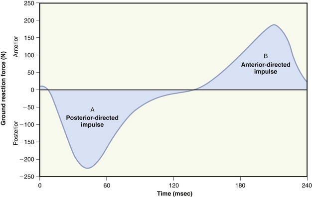
Numerically, an impulse can be calculated as the product of the average force (N) and its time of application. Impulse can also be represented graphically as the area under a force-time curve. Figure 4-4 displays a force-time curve of the horizontal component of the anterior-posterior shear force applied by the ground against the foot (ground reaction force) as an individual runs across a force plate embedded in the floor. The curve is biphasic: the posterior-directed impulse during initial floor contact is negative, and the anterior-directed impulse during propulsion is positive. If the two impulses (i.e., areas under the curves) are equal, the net impulse is zero, and there is no change in the momentum of the system. In this example, however, the posterior-directed impulse is greater than the anterior, indicating that the runner’s forward momentum is decreased.
Work-Energy Relationship: To this point, Newton’s second law has been described using (1) the force (torque)-acceleration relationship (Equations 4.1 and 4.3) and (2) the impulse-momentum relationship (Equations 4.4 through 4.7). Newton’s second law can also be restated to provide a work-energy relationship. This third approach can be used to study human movement by analyzing the extent to which work causes a change in an object’s energy. Work occurs when a force or torque operates over some linear or angular displacement. Work (W) in a linear sense is equal to the product of the magnitude of the force (F) applied against an object and the linear displacement of the object in the direction of the applied force (Equation 4.8). If no movement occurs in the direction of the applied force, no mechanical work is done. Similar to the linear case, angular work can be defined as the product of the magnitude of the torque (T) applied against the object, and the angular displacement of the object in the direction of the applied torque (Equation 4.9). Work is expressed in joules (J).
 Positive Work, Negative Work, and “Isometric Work”


Average power (P) is work (W) divided by time (Equation 4.10). Because work is the product of force (F) and displacement (d), the rate of work at any instant can be restated in Equation 4.11 as the product of force and velocity. Angular power may also be defined as in the linear case, using the angular analogs of force and linear velocity: torque (T) and angular velocity (ω), respectively (Equation 4.12). Angular power is often used as a clinical measure of muscle performance. The mechanical power produced by the quadriceps, for example, is equal to the net internal torque produced by the muscle times the average angular velocity of knee extension. Power is often used to designate the net transfer of energy between active muscles and external loads. Positive power reflects the rate of work done by concentrically active muscles against an external load. Negative power, in contrast, reflects the rate of work done by the external load against eccentrically active muscles.

Table 4-2 summarizes the definitions and units needed to describe many of the physical measurements related to Newton’s second law.
TABLE 4-2.
Physical Measurements Associated with Newton’s Second Law
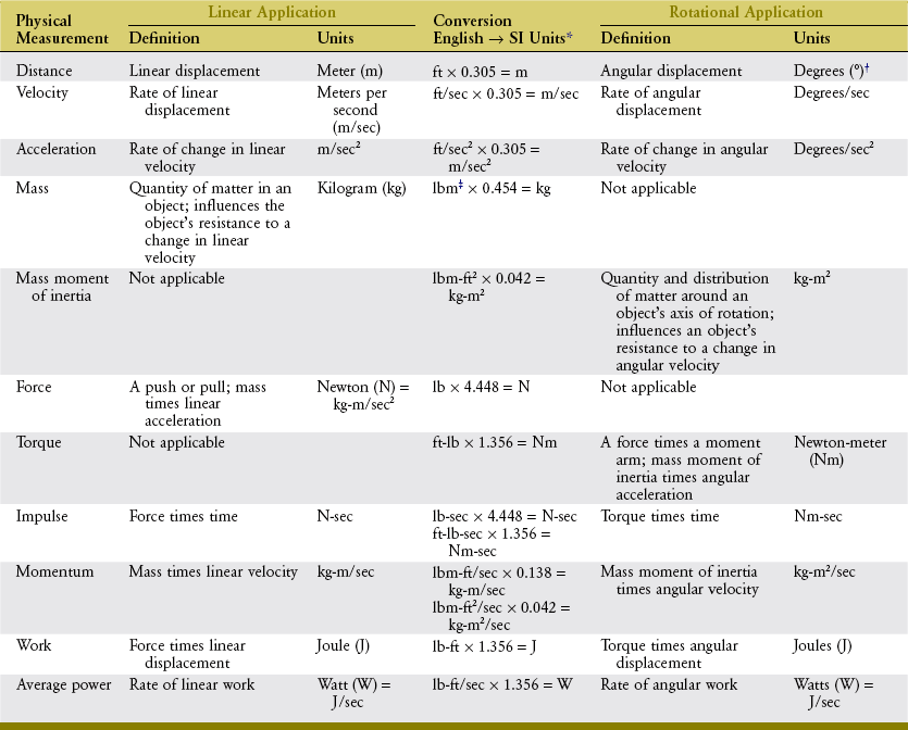
*To convert from English units to SI units, multiply the English value by the number in the table cell. To convert from SI units to English, divide by that number. If two equations are in the cell, the upper equation is used to convert the linear measure, and the lower equation is used to convert the angular measure.
†Radians, which are unitless, may be used instead of degrees (1 radian = about 57.3 degrees).
NEWTON’S THIRD LAW: LAW OF ACTION-REACTION
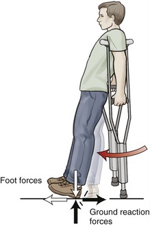
Another example of Newton’s law of action-reaction is the reaction force provided by the surface on which one is walking or standing. The foot produces a force against the ground, and in accordance with Newton’s third law, the ground generates a ground reaction force in the opposite direction but of equal magnitude (Figure 4-5). The ground reaction force changes in magnitude, direction, and point of application on the foot throughout the stance period of gait. Newton’s third law also has an angular equivalent. For example, during an isometric exercise, the internal and external torques are equal and in opposite rotary directions.
INTRODUCTION TO MOVEMENT ANALYSIS: SETTING THE STAGE FOR ANALYSIS
Anthropometry
Much of the information pertaining to the body segments’ center of gravity and mass moment of inertia has been derived from cadaver studies.3,4 Other methods for deriving anthropometric data include mathematic modeling and imaging techniques, such as computed tomography and magnetic resonance imaging. Table 4-3 lists data on the weights of body segments and the location of the center of gravity. (The specific details contained in this table will be needed to solve selected parts of the biomechanical problems posed in Appendix I, Part B).
TABLE 4-3.
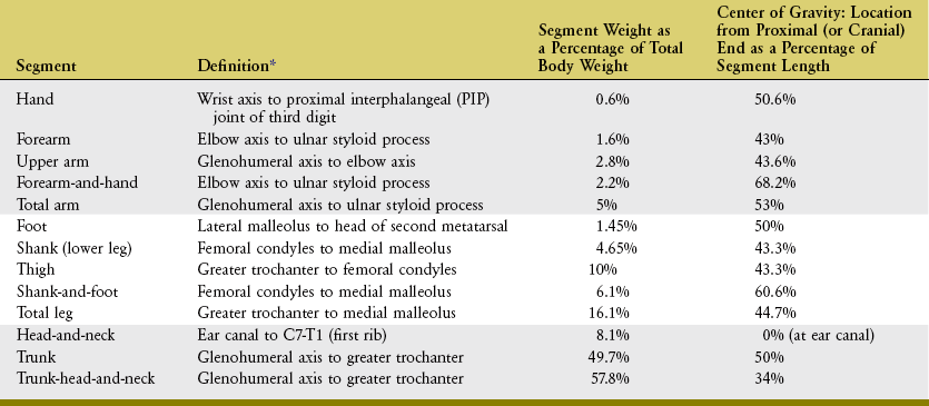
*Even though some definitions listed in this table do not represent the endpoints of the segment, they are easily identified locations on the human. The values for segment weight and center of gravity location in this table take into consideration the discrepancy between the definition of the segment and the true endpoints. For example, the segment definition for the forearm is the same for the forearm-and-hand, but the percentages listed for the segment weight and center of gravity location of the forearm-and-hand are higher, taking into consideration the mass of the hand.
Free Body Diagram
How a free body diagram is configured depends on the intended purpose of the analysis. Consider the example presented in Figure 4-6. In this example, the free body diagram represents the shank-and-foot at the instant of initial heel contact during walking. The free body diagram involves figuratively “cutting through” the desired joint(s) to isolate or “free” the body of interest. In the example presented in Figure 4-6, the knee joint was cut through to isolate the shank-and-foot segment. The effects of active muscle force are usually distinguished from the effects of other soft tissues, such as passive tension created in stretched joint capsule and ligaments. Although the contribution of individual muscles acting across a joint may be determined, a single resultant muscle force (M) vector is often used to represent the sum total of all individual muscle forces. Other forces external to the system are added to the diagram, which may include the ground reaction force (G) and weight of the shank-and-foot segments (S and F). As specified by Newton’s third law, the ground reaction force is the force developed in response to the foot striking the earth.
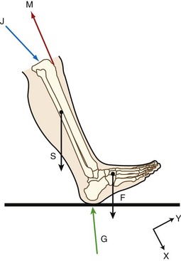
An additional force is identified in Figure 4-6: the joint reaction force (J). This force includes joint contact forces as well as the net or cumulative effect of all other forces transmitted from one segment to another. Joint reaction forces are caused “in reaction” to other forces, such as those produced by activation of muscle, by passive tension in stretched periarticular connective tissues, and by gravity (body weight). As will be discussed, the free body diagram is completed by defining an X-Y coordinate reference frame and writing the governing equations of motion.
Clinically, reducing joint reaction force is often a major focus in treatment programs designed to lessen pain and prevent further joint degeneration in persons with arthritis. Frequently, treatments are directed toward reducing joint forces through changes in the magnitude of muscle activity and their activation patterns or through a reduction in the weight transmitted through a joint. Consider the patient with osteoarthritis of the hip joint as an example. The magnitude of the hip joint’s reaction force may be decreased by having the person reduce walking velocity, thereby lessening the magnitude of muscle activation. Highly cushioned shoes may be recommended to reduce impact forces. In addition, a cane may be used to reduce forces through the hip joint.1,10,13 If obesity is a factor, a weight-reduction program may be recommended.
STEPS FOR CONSTRUCTING THE FREE BODY DIAGRAM
Consider the situation in which an individual is holding a weight out to the side, as shown in Figure 4-7. This free body is assumed to be in static equilibrium, and the sum of all forces and the sum of all torques acting on the body are equal to zero. One purpose of the analysis might be to determine how much muscle force is required by the glenohumeral joint abductor muscles (M) to keep the arm abducted to 90 degrees; another purpose might be to determine the magnitude of the glenohumeral joint reaction force (J) during this same activity.
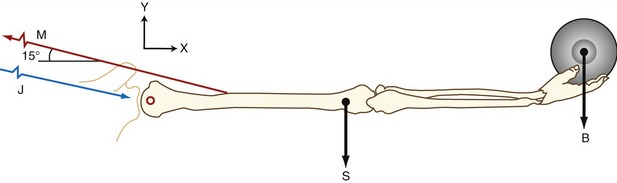
Step II involves defining a coordinate reference frame that allows the position and movement of a body to be defined with respect to a known point, location, or axis (see Figure 4-7, X-Y coordinate reference frame). More detail on establishing a reference frame is discussed ahead.
Step III involves identification and inclusion of all forces that act on the free body. Internal forces are those produced by muscle (M). External forces include the force of gravity on the mass of the exercise ball (B), as well as the force of gravity on the arm segment (S). Although not relevant to Figure 4-7, other examples of external forces could include forces applied by therapists, cables, resistance bands, the ground or other surface, air resistance, and orthotics. The forces are drawn on the figure while specifying their approximate point of application and spatial orientation. For example, vector S acts at the center of gravity of the upper extremity, a location determined by using anthropometric data, such as those presented in Table 4-3.
SPATIAL REFERENCE FRAMES
Whether motion is measured via a relative or global reference frame, the location of a point or segment in space can be specified using a coordinate reference frame. In laboratory-based human movement analysis, the Cartesian coordinate system is most frequently employed. The Cartesian system uses coordinates for locating a point on a plane in 2D space by identifying the distance of the point from each of two intersecting lines, or in three-dimensional (3D) space by the distance from each of three planes intersecting at a point. A 2D coordinate reference frame is defined by two imaginary axes arranged perpendicular to each other with the arrowheads pointed in positive directions. The two axes (labeled, for example, X and Y) may be oriented in any manner that facilitates quantitative solutions (compare Figures 4-6 and 4-7, for example). A 2D reference frame is frequently used when the motion being described is predominantly planar (i.e., in one plane), such as knee flexion and extension during gait.
In most cases, human motion occurs in more than one plane. In order to fully describe this type of motion, a 3D coordinate reference frame is necessary. A 3D reference frame typically has three axes (X, Y, and Z), each perpendicular (or orthogonal) to another. As with the 2D system, the arrowheads point in positive directions. A universal convention for orienting this triplanar coordinate system in space is based on the right-hand rule. This rule is used throughout most quantitative biomechanical studies (see Special Focus 4-4).
Throughout most of this textbook, the terminology used to describe linear direction within planes (such as the direction of a muscle force or an axis of rotation around a joint) is less formal than that dictated by the right-hand rule. As described in Chapter 1, linear direction in space is loosely described relative to the human body standing in the anatomic position, using terms such as anterior-posterior, medial-lateral, and vertical. Although useful for most qualitative or anatomic-based descriptions, this convention is not well suited for quantitative analyses, such as those introduced later in this chapter. In these cases, the Cartesian coordinate system is used, and the orientation of its 3D axes is designated by the right-hand rule.
SPECIAL FOCUS 4-4  The “Right-Hand Rule”: a Convention for Completely Describing the Spatial Orientation of a Three-Dimensional Coordinate Reference Frame
When a Cartesian coordinate system is set up, the direction or orientation of the orthogonal axes is not arbitrary. A convention must be used to facilitate the sharing of research from different laboratories throughout the worldwide scientific community. Using Figure 4-7 as an example, the X and Y axes are in the plane of the page or, relative to the subject, parallel with the frontal plane. (It is often most convenient, although not mandatory, to orient the X-Y axes so that the X axis is parallel with the body segment of interest.) A third axis, the Z axis, must be defined. Although not drawn in the figure, the Z axis is oriented perpendicular to the X-Y plane. By convention, the direction of the arrowheads shown on the X-Y coordinate reference frame indicates positive directions. As shown in Figure 4-7, positive X direction is to the right and positive Y direction is upward. The right-hand rule can be used to define the direction (+ or −) of the Z axis. Applying the right-hand rule is performed by laying the ulnar border of your right hand along the X axis, with the straight fingers pointing in a positive X direction (toward the ball on the model). Your hand should be positioned along the X axis so that when your fingers flex, they curl from the positive X direction toward the positive Y direction. Your extended thumb is pointing out of the page, thereby defining the direction of the positive Z axis. By necessity, the −Z axis is oriented perpendicularly into the page. Using the right-hand rule means that only two axes ever need to be defined and shown; use of the right-hand rule allows the third axis to be completely described.
SPECIAL FOCUS 4-5  Another Use of the “Right-Hand Rule”: a Guide for Describing the Direction of Angular Motion and Torque
Another use of the right-hand rule is to define the rotation direction of angular motion and torque. Consider once again, the coordinate reference frame depicted in Figure 4-7. This reference frame indicates that the path of humeral motion (abduction) is in the X-Y (frontal) plane, around a perpendicular anterior-posterior axis (or, as described in Special Focus 4-4, the Z axis). The right-hand rule is again applied to Figure 4-7 as follows. Begin by aligning the ulnar side of your right hand parallel with the arm segment of the model, so that flexing your fingers curls them in the rotation path of shoulder abduction. The direction of your extended thumb points in the +Z direction, indicating abduction is a positive Z rotation. Shoulder adduction is in a negative Z direction.
This right-hand rule is also used to describe the rotary direction of torque. Again the right hand is used, curling your fingers in the path of motion produced by the torque. Returning to Figure 4-7, force M, produced by the shoulder abductor muscles, generates a +Z torque, whereas the shoulder adductor muscles (not shown) generate a −Z torque. With the coordinate reference frame oriented as shown, the shoulder abductors will always generate a +Z torque, regardless of concentric action (associated with a +Z motion), or eccentric action (associated with a −Z motion).
Rotary or angular movements or torques are often described as occurring in a plane, around a perpendicular axis of rotation. In most kinesiologic literature, a segment’s rotation direction is typically described by terms such as flexion and extension and, to a lesser extent, clockwise or counterclockwise rotation. Such a system is adequate for most clinical analysis and is used throughout this textbook. More formal, quantitative analysis, however, may be necessary to designate the direction of angular motion and torques. Such a system is based on the 3D Cartesian coordinate reference frame and uses another form of the right-hand rule,4 as described in Special Focus 4-5.
In closing, analyzing movement within three dimensions is more complicated than in two dimensions, but it does provide a more comprehensive profile of human movement. There are excellent resources available that describe techniques for conducting 3D analysis, and some of these references are provided at the end of the chapter.2,22,23 The quantitative analysis described in this chapter focuses on movements that are restricted to two dimensions.
Forces and Torques
GRAPHIC AND MATHEMATIC METHODS OF FORCE ANALYSIS
The trigonometric method does not require the same precision of drawing, and often provides a more accurate method of force analysis. This method uses rectangular components, and “right-angle trigonometry” to determine magnitudes and angles of forces. The trigonometric functions are based on the relationship that exists between the angles and sides of a right triangle. Refer to Appendix I, Part A, for a brief review of this material.
Composition of Forces: Two or more forces are collinear if they share a common line of force. Vector composition allows several collinear forces to be simply combined graphically as a single resultant force (Figure 4-8). In Figure 4-8, A, the weight of the shank-and-foot segments (S) and the exercise weight (W) are added graphically by means of a ruler and a scale factor determined for the vectors. In this example, S and W act downward, so the resultant force (R) also acts downward and has the tendency to distract (pull apart) the knee joint. R is found graphically by aligning the tail of W to the tip of S. The resultant force R is depicted by the blue arrow that starts at the tail of S and ends at the tip of W. Figure 4-8, B illustrates a cervical traction device that employs a weighted pulley system, acting upward, opposite to the force created by gravity on the center of gravity of the head. Graphically, the tail of H is aligned to the tip of T, and the resultant arrow (R) starts at the tail of T and ends at the tip of H. The upward direction of R (in blue) indicates a net upward distraction force on the head and neck.
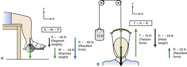
The collinear forces depicted in Figure 4-8 can also be combined by simply adding the force magnitudes of the vectors while paying attention to their directions. In Figure 4-8, A, the coordinate reference frame indicates both S and W are collinear and both acting entirely in a −Y direction. As indicated in the box, the result is found by adding the magnitudes of the collinear forces; in this case the result also acts in a −Y direction. In Figure 4-8, B, the forces are collinear but acting in opposite directions (T acting in a +Y direction, H acting in a −Y direction). Adding the two magnitudes together while paying attention to the direction indicates the result is a 22 N force acting in a +Y direction. In this specific example, a traction force of at least 53 N is needed to offset the weight of the head. Using less force would result in no actual distraction (separation) or the cervical vertebrae. This technique may still, however, provide some therapeutic benefit.
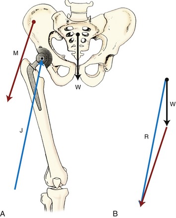
Forces acting on a body may be coplanar (in the same plane), but they may not always be collinear. In this case the individual force vectors may be composed graphically using the polygon method. Figure 4-9 illustrates how the polygon method can be applied to a frontal plane model to estimate the joint reaction force on a prosthetic hip while the subject is standing on one limb. With the arrows drawn in proportion to their magnitude and in the correct orientation, the vectors of body weight (W) and hip abductor muscle force (M) are added in a tip-to-tail fashion (see Figure 4-9, B). The combined effect of the W and M vectors is determined by placing the tail of the M vector to the tip of the W vector. Completing the polygon yields the resultant force (R) starting at the tail of W and traveling to the tip of M. Figure 4-9, B illustrates this process, indicating the magnitude and direction of R. Note that R is equal in magnitude, but opposite in direction, to the prosthetic hip joint reaction force (J) depicted in Figure 4-9, A. An excessively large joint reaction force may, over time, contribute to premature loosening of the hip prosthesis.
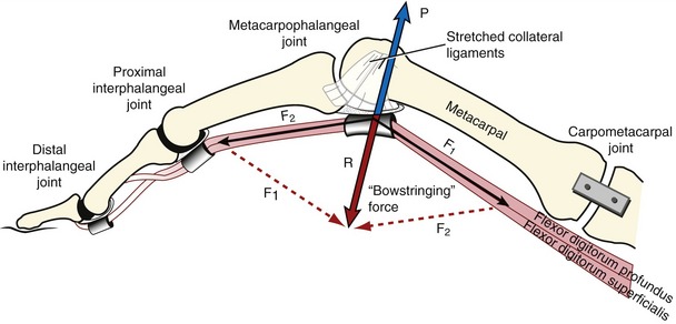
A parallelogram can also be constructed to determine the resultant of two coplanar but noncollinear forces. Instead of placing the force vectors tip to tail, as discussed in the previous example, the resultant vector can be found by drawing a parallelogram based on the magnitude and direction of the two component force vectors. As with all graphic techniques of vector analysis, practice is required to be able to relatively accurately draw the size and orientation of the associated force vectors. Figure 4-10 provides an illustration of the parallelogram method used to combine several component vectors into one resultant vector. The component force vectors, F1 and F2 (black solid arrows), are generated by the pull of the flexor digitorum superficialis and profundus as they pass palmar (anterior) to the metacarpophalangeal joint. The diagonal, originating at the intersection of F1 and F2, represents the resultant force (R) (see Figure 4-10, thick red arrow). Because of the angle between F1 and F2, the resultant force tends to raise the tendons palmarly away from the joint. Clinically, this phenomenon is described as a bowstringing force because of the tendons’ resemblance to a pulled cord connected to the two ends of a bow. Normally the bowstringing force is resisted by forces developed in the flexor pulley and collateral ligaments (see force P in blue in Figure 4-10). In severe cases of rheumatoid arthritis, for example, the bowstringing force may eventually rupture the ligaments and dislocate the metacarpophalangeal joints.
Resolution of Forces: The previous section illustrates the composition method of representing forces, whereby multiple coplanar forces acting on a body are replaced by a single resultant force. In many clinical situations, however knowledge of the effect of the individual components that produce the resultant force may be more relevant to understanding the impact of these forces on motion and joint loading, as well as developing specific treatment strategies. Vector resolution is the process of replacing a single force with two or more forces that when combined are equivalent to the original force.
One of the most useful applications of the resolution of forces involves the description and calculation of the rectangular components of a muscle force. As depicted in Figure 4-11, the rectangular components of the muscle force are shown at right angles to each other and are referred to as the X and Y components (MX and MY). (The X axis is set to be parallel to the long axis of the segment, with positive directed distally.) In the elbow model depicted in Figure 4-11, the X component represents the component of the muscle force that is directed parallel to the forearm. The effect of this force component is to compress and stabilize the joint or, in some cases, distract or separate the segments forming the joint. The X component of a muscle force does not produce a torque when it passes through the axis of rotation because it has no moment arm (see Figure 4-11, MX). In the model depicted in Figure 4-11, the Y component represents the component of the muscle force that acts perpendicularly to the long axis of the segment. Because of the internal moment arm (see Chapter 1) associated with this force component, one effect of MY is to cause a rotation (i.e., produce a torque). In this example, the MY component may also create a shear force at the humeroradial joint that tends to cause a translation of the bony segment in the +Y direction.
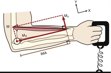
For the purposes of this chapter, anatomic joints will be considered as frictionless hinge or pin joints with a stationary axis of rotation, allowing rotation in only one plane. Although it is fully recognized that even the simplest joint in the body is far more complex than this, consideration as pin joints allows a much easier understanding of the concepts of this chapter. For example, if the X component of the muscle force (MX) is directed toward the elbow joint as in Figure 4-11, it may be assumed that the muscle force causes compression of the radial head against the capitulum of the humerus. The Y component of the muscle force (MY in Figure 4-11) causes a shear, tending to move the forearm in the +Y direction (in this case upward and slightly posteriorly). As described later, these forces are opposed by the oppositely directed joint reaction forces. Table 4-4 summarizes the characteristics of the X and Y force components of a muscle, as illustrated in Figure 4-11.
TABLE 4-4.
Typical Characteristics of X and Y Components of a Muscle Force (as Illustrated in Figure 4-11)
| Y Muscle Force Component | X Muscle Force Component |
| Acts perpendicular to a bony segment. | Acts parallel to a bony segment. |
| Often indicated as MY, depending on the choice of the reference system. | Often indicated as MX, depending on the choice of the reference system. |
| Can cause translation of the bone and/or torque if moment arm >0. | Can cause translation of the bone. Often does not cause a torque because the chosen reference system reduces the moment arm to zero. |
| In a simple hinge joint model, MY creates a shear force between the articulating surfaces. (In reality, MY can create shear, compressive, and distractive forces depending on the anatomic complexity of the joint surfaces.) | In a simple hinge joint model, MX creates a compression or distraction force between the articulating surfaces. (In reality, MX can create shear, compressive, and distractive forces depending on the anatomic complexity of the joint surfaces.) |
CONTRASTING INTERNAL VERSUS EXTERNAL FORCES AND TORQUES
The previously described examples of resolving forces into X and Y components focused on the forces and torques produced by muscle. As described in Chapter 1, muscles, by definition, produce internal forces and torques. The resolution of forces into X and Y components can also be applied to external forces acting on the human body, such as those from gravity, physical contact, external loads and weights, and manual resistance as applied by a clinician. In the presence of an external moment arm, external forces produce an external torque. Generally, in a condition of equilibrium the external torque acts relative to the joint’s axis of rotation in an opposite rotary direction as the net internal torque.
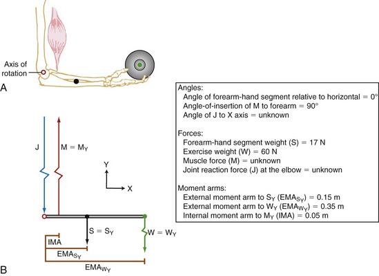
Figure 4-12 illustrates the resolution of both internal and external forces of an individual who is performing an isometric knee extension exercise. Three forces are depicted in Figure 4-12, A: the internal knee extensor muscle force (M), the external shank-and-foot segment weight (S), and the external exercise weight (W) applied at the ankle. Forces S and W act at the center of their respective masses.
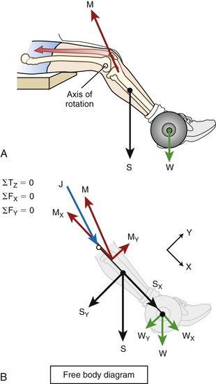
Figure 4-12, B shows the free body diagram of the exercise performed in A, with M, S, and W resolved into their X and Y components. Assuming static rotary and linear equilibrium, the governing torque (T) and force (F) equations listed to the left of the figure may be used to solve unknown variables. This topic will be addressed in the final section of the chapter.
INFLUENCE OF CHANGING THE ANGLE OF THE JOINT
The relative magnitude of the X and Y components of internal and external forces applied to a bone depends on the position of the limb segment. Consider first how the change in angular position of a joint alters the angle-of-insertion of the muscle (see glossary, Chapter 1). Figure 4-13 shows the constant magnitude biceps muscle force (M) at four different elbow joint positions, each with a different angle-of-insertion to the forearm (designated as α in each of the four parts of the figure). Note that each angle-of-insertion results in a different combination of MX and MY force components. The MX component creates compression force if it is directed toward the elbow, as in Figure 4-13, A, or distraction force if it is directed away from the elbow as in Figure 4-13, C and D. By acting with an internal moment arm (brown line labeled IMA), the MY components in Figure 4-13, A through D generate a +Z torque (flexion torque) at the elbow.
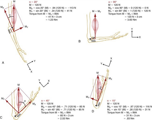
As shown in Figure 4-13, A, a relatively small angle-of-insertion of 20 degrees favors a relatively large X component force, which directs a larger percentage of the total muscle force to compress the joint surfaces of the elbow. Because the angle-of-insertion is less than 45 degrees in Figure 4-13, A, the magnitude of the MX component exceeds the magnitude of the MY component. When the angle-of-insertion of the muscle is 90 degrees (as in Figure 4-13, B), 100% of M is in the Y direction and is available to produce an elbow flexion torque. At an angle-of-insertion of 45 degrees (Figure 4-13, C), the MX and MY components have equal magnitude, with each about 71% of M. In Figure 4-13, C and D, the angle-of-insertion (shown to the right of M as α) produces a MX component that is directed away from the joint, thereby producing a distracting or separating force on the joint.
In Figure 4-13, A through D, the internal torque is always in a +Z direction and is the product of MY and the internal moment arm (IMA). Even though the magnitude of M is assumed to remain constant throughout the range of motion, the change in MY (resulting from changes in angle-of-insertion) produces differing magnitudes of internal torque. Note that the +Z (flexion) torque ranges from 0.93 Nm at near full elbow flexion to 3.60 Nm at 90 degrees of elbow flexion—a near fourfold difference. This concept helps explain why people have greater strength (torque) in certain parts of the joint’s range of motion. The torque-generating capabilities of the muscle depend not only on the angle-of-insertion, and subsequent magnitude of MY, but also on other physiologic factors, discussed in Chapter 3. These include muscle length, type of activation (i.e., isometric, concentric, or eccentric), and velocity of shortening or elongation of the activated muscle.
Changes in joint angle also can affect the amount of external or “resistance” torque encountered during an exercise. Returning to the example of the isometric knee extension exercise, Figure 4-14 shows how a change in knee joint angle affects the Y component of the external forces S and W. The external torque generated by gravity on the segment (S) and the exercise weight (W) is equal to the product of the external moment arm (brown line labeled EMA in B and C) and the Y component of the external forces (SY and WY). In Figure 4-14, A, no external torque exists in the sagittal plane because S and W force vectors are entirely in the +X direction (SY and WY = 0). The S and W vectors are directed through the knee’s axis of rotation and therefore have no external moment arm. Because these external forces are pointed in the +X direction, they tend to distract the joint. Figure 4-14, B and C show how a greater external torque is generated with the knee fully extended (in C) compared with the knee flexed 45 degrees (in B). Although the magnitude of the external forces, S and W, are the same in all three cases, the −Z directed (flexion) external torque is greatest when the knee is in full extension. As a general principle, the external torque around a joint is greatest when the resultant external force vector intersects the bone or body segment at a right angle (as in Figure 4-14, C). When free weights are used, for example, external torque is generated by gravity acting vertically. Resistance torque from the weight is therefore greatest when the body segment is positioned horizontally. Alternatively, with use of a cable attached to a column of stacked weights, resistance torque from the cable is greatest in the position where the cable acts at a right angle to the segment. Note that this is often in a different position than where the torque caused by gravity acting on the segment is greatest. Resistive elastic bands and tubes present further complications, as resistance torque from these devices varies with the angle of the resistance force vector and the amount of stretch in the device; both factors vary through a range of motion.19,21
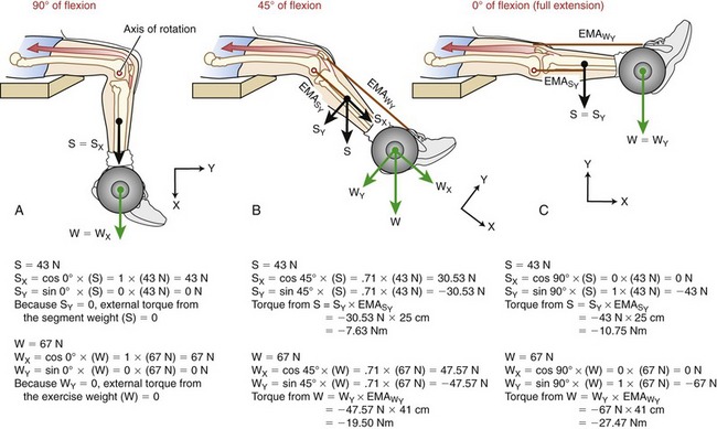
 is equal to the external moment arm for SY;
  is equal to the external moment arm for WY). Different external torques are generated at each of the three knee angles. The X-Y coordinate reference frame is set so the X direction is parallel to the shank segment; thin black arrowheads point toward the positive direction.
SPECIAL FOCUS 4-6  Designing Resistive Exercises So That the External and Internal Torque Potentials Are Optimally Matched
The concept of altering the angle of a joint is frequently used in exercise programs to adjust the magnitude of resistance experienced by the patient or client. It is often desirable to design an exercise program so that the external torque matches the internal torque potential of the muscle or muscle group. Consider a person performing a “biceps curl” exercise, shown in Figure 4-17, A. With the elbow flexed to 90 degrees, both the internal and external torque potentials are greatest, because the product of each resultant force (M and W) and their moment arms (IMA and EMA) are maximal. At this elbow position the internal and external torque potentials are maximal as well as optimally matched. As the elbow position is altered in Figure 4-17, B, the external torque remains the same; however, the angle-of-insertion of the muscle is different, requiring a much larger muscle force, M, to produce the same internal +Z directed torque. Note the Y component of the muscle force (MY) in Figure 4-17, B has the same magnitude as the muscle force M in Figure 4-17, A. A person with significant weakness of the elbow flexor muscle may have difficulty holding an object in position B but may have no difficulty holding the same object in position A.
COMPARING TWO METHODS FOR DETERMINING TORQUE AROUND A JOINT
Internal Torque: The two methods for determining internal torque are illustrated in Figure 4-15. Method 1 calculates the internal torque as the product of MY and its internal moment arm ( ). Method 2 uses the entire muscle force (M) and therefore does not require this variable to be resolved into its rectangular components. In this method, internal torque is calculated as the product of the muscle force (the whole force, not a component) and IMAM (i.e., the internal moment arm that extends perpendicularly between the axis of rotation and the line of action of M). Methods 1 and 2 yield the same internal torque because they both satisfy the definition of a torque (i.e., the product of a force and its associated moment arm). The associated force and moment arm for any given torque must intersect each other at a 90-degree angle.
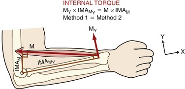
 ). Method 2 calculates torque as the product of the entire force of the muscle (M) times its internal moment arm (IMAM). Both expressions yield equivalent internal torques. The axis of rotation is depicted as the open black circle at the elbow. The X-Y coordinate reference frame is set so the positive X direction is parallel to the forearm segment.
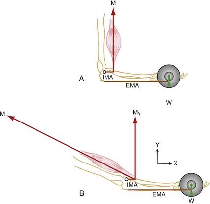
External Torque: Figure 4-16 shows an external torque applied to the elbow through a resistance produced by an elastic band (depicted in green as R). The weight of the body segment is ignored in this example. Method 1 determines external torque as the product of RY times its external moment arm ( ). Method 2 uses the product of the band’s entire resistive force (R) and its external moment arm (EMAR). As with internal torque, both methods yield the same external torque because both satisfy the definition of a torque (i.e., the product of a resistance [external] force and its associated external moment arm). The associated force and moment arm for any given torque must intersect each other at a 90-degree angle.
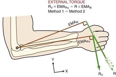
 ). Method 2 calculates torque as product of the entire force of the resistance (R) times its external moment arm (EMAR). Both expressions yield equivalent external torques. The axis of rotation is depicted as the open black circle at the elbow. The X-Y coordinate reference frame is set so the positive X direction is parallel to the forearm segment.
MANUALLY APPLYING EXTERNAL TORQUES DURING EXERCISE AND STRENGTH TESTING
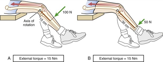
Because external torque is the product of a force (resistance) and an associated external moment arm, an equivalent external torque can be applied by a relatively short external moment arm and a large external force, or a long external moment arm and a smaller external force. The knee extension resistance exercise depicted in Figure 4-18 shows that the same external torque (15 Nm) can be generated by two combinations of external forces and moment arms. Note that the resistance force applied to the leg is greater in Figure 4-18, A than in Figure 4-18, B. The higher contact force may be uncomfortable for the patient, and this factor needs to be considered during the application of resistance. A larger external moment arm, as shown in Figure 4-18, B, may be necessary if the clinician chooses to manually challenge a muscle group as potentially forceful as the quadriceps. Even using a long external moment arm, clinicians may be unable to provide enough torque to maximally resist large and strong muscle groups.11
A hand-held dynamometer is a device used to manually measure the maximal isometric strength of certain muscle groups. This device directly measures the force generated between the device and the limb during a maximal-effort muscle contraction. Figure 4-19 shows this device used to measure the maximal-effort, isometric elbow extension torque in an adult woman. The external force (R) measured by the dynamometer is in response to the internal force generated by the elbow extensor muscles (E). Because the test is performed isometrically, the measured external torque (R × EMA) will be equal in magnitude but opposite in direction to the actively generated internal torque (E × IMA). If the clinician is documenting external force (as indicated by the dial on the dynamometer), he or she needs to pay close attention to the position of the dynamometer relative to the person’s limb. Changing the external moment arm of the device will alter the external force reading. This is shown by comparing the two placements of the dynamometer in Figure 4-19, A and B. The same elbow extension internal force (E) will result in two different external force readings (R). The longer external moment arm used in Figure 4-19, A, results in a lower external force than the shorter external moment arm used in Figure 4-19, B. On repeated testing, for example, before and after a strengthening program, the force dynamometer must be positioned with exactly the same external moment arm to allow a valid strength comparison to the prestrengthening values. Documenting external torques rather than forces does not require the external moment arm to be exactly the same for every testing session. The external moment arm does need to be measured each time, however, to allow conversion of the external force (as measured by the force dynamometer) to external torque (the product of the external force and the external moment arm).
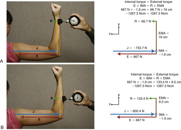
FIGURE 4-19. A dynamometer is used to measure the maximal, isometric strength of the elbow extensor muscles. The external moment arm (EMA) is the distance between the axis of rotation (open circle) and the point of external force (R) measured by the dynamometer. The different placement of the device on the limb creates different EMAs in A and B. Elbow extension force (E), which is the same in A and B, generates equivalent internal torques through its internal moment arm (IMA), which is equal in magnitude but opposite in direction to the external torques generated by the product of R and EMA. The joint reaction force (J), shown in blue, is equal but opposite in direction to the sum of R + E. The distal application of the measuring device shown in A results in a longer EMA and a lower external force reading. Because R is less, J is also less. The more proximal application of the device in B results in a shorter EMA, a higher external force reading, and a greater J. Vectors are drawn to approximate scale. (The X-Y coordinate reference frame is set so the X direction is parallel to the forearm; thin black arrowheads point in positive directions. Based on conventions described in the next section [summarized in Box 4-1], the internal moment arm is assigned a negative number. This, in turn, appropriately assigns opposite rotational directions to the opposing torques.)
Note also that although the elbow extension internal force and torque are the same in Figure 4-19, A and B, the joint reaction force (J) and external force (R) are higher in Figure 4-19, B. This means that the pressure between the force dynamometer pad and the patient’s skin is higher and could potentially cause discomfort. In some cases the discomfort could be great enough to reduce the amount of internal torque the patient is willing to develop, thereby influencing a maximal strength assessment. In addition, a higher magnitude of joint reaction force could have implications in conditions of compromised articular cartilage.
INTRODUCTION TO BIOMECHANICS: FINDING THE SOLUTIONS
Static Analysis
The force equilibrium equations, Equations 4.13 A and B, are used for static (uniplanar) translational equilibrium. In the case of static rotational equilibrium, the sum of the torques around any axis of rotation is zero. The torque equilibrium equation, Equation 4.14, is also included. The equations previously depicted in Figure 4-19 provide a simplified example of static rotational equilibrium about the elbow. The muscle force of the elbow extensors (E) times the internal moment arm (IMA) creates a potential extension (clockwise, −Z) torque. This torque (product of E and IMA) is balanced by a flexion (counterclockwise, +Z) torque provided by the product of the transducer’s force (R) and its external moment arm (EMA). Assuming no movement of the elbow, ΣTZ = 0; in other words, the opposing torques at the elbow are assumed to be equal in magnitude and opposite in direction.
Governing Equations for Static Uniplanar Analysis
Forces and Torques Are Balanced
Force (F) Equilibrium Equations


GUIDELINES FOR PROBLEM SOLVING
The guidelines listed in Box 4-1 are necessary to follow the logic for solving the upcoming three sample problems. (Although most concepts listed in Box 4-1 have been described previously in this chapter, guideline 5 is new. This particular guideline describes the convention used to assign direction to moment arms.) In each of the three upcoming problems, an assumption of static equilibrium is required to solve the magnitude and direction of torque, muscle force, and joint reaction force.
Additional problem-solving examples and related clinical questions are available in Appendix I, Part B.
Problem 1: Consider the situation posed in Figure 4-20, A, in which a person generates an isometric elbow flexor muscle force at the elbow while holding a weight in the hand. Assuming equilibrium, the three unknown variables are the (1) internal (muscle-produced) elbow flexion torque, (2) elbow flexor muscle force, and (3) joint reaction force at the elbow. All abbreviations and pertinent data are included in the box associated with Figure 4-20.
To begin, a free body diagram and X-Y reference frame is constructed (see Figure 4-20, B). The axis of rotation and all moment arm distances are indicated. Although at this point the direction of the joint (reaction) force (J) is unknown, it is assumed to act in a direction opposite to the pull of muscle. This assumption generally holds true in an analysis in which the mechanical advantage of the system is less than one (i.e., when the muscle forces are greater than the external resistance forces) (see Chapter 1).
Resolving Known Forces into X and Y Components: In the elbow position depicted in Figure 4-20, all forces act parallel to the Y axis; there is no force acting in the X direction. This means the magnitude of the Y components of the forces is equal to the magnitude of the entire force, and the X components are all zero. This situation is unique to this position, in which muscle force and gravity are vertical and the segment is positioned horizontally.
Solving for Internal Torque and Muscle Force: The external torques originating from the weight of the forearm-hand segment (SY) and the exercise weight (WY) generate a −Z (clockwise, extension) torque about the elbow. In order for the system to remain in equilibrium, the elbow flexor muscles have to generate an opposing internal +Z (counterclockwise, flexion) torque. Summing the torques around the elbow axis allows the line-of-action of J to pass through the axis, thus making the moment arm of J equal to zero. This results in only one unknown in Equation 4.14: the magnitude of the muscle force:


Solving for Joint Reaction Force: Because the joint reaction force (J) is the only remaining unknown variable depicted in Figure 4-20, B, this variable is determined by Equations 4.13 A and B.


Because muscle force is usually the largest force acting about a joint, the direction of the net joint reaction force often opposes the pull of the muscle. Without such a force, for example, the muscle indicated in Figure 4-20 would accelerate the forearm upward, resulting in an unstable joint. In short, the joint reaction force in this case (largely supplied by the humerus pushing against the trochlear notch of the ulna) provides the required force to maintain linear static equilibrium at the elbow. As stated earlier, the joint reaction force does not produce a torque because it is assumed to act through the axis of rotation and therefore has a zero moment arm.
Clinical Questions Related to Problem 1:
1. Assume a patient with osteoarthritis of the elbow is holding a load similar to that depicted in Figure 4-20. How would you respond to the question posed by a patient, “Why would my elbow be so painful from holding such a light weight?”
2. Describe a few clinical conditions in which the magnitude and direction of the joint reaction force could be biomechanically (physiologically) unhealthy for a patient.
3. Which variable is most responsible for the magnitude and direction of the joint reaction force at the elbow?
4. Assume a person with a recent elbow joint replacement needs to strengthen the elbow flexor muscles. Given the isometric situation depicted in Figure 4-20:
Answers to the clinical questions can be found on the Evolve website. 
Problem 2: In Problem 1 the forearm is held horizontally, thereby orienting the internal and external forces perpendicular to the forearm. Although this presentation greatly simplifies the calculations, it does not represent a typical biomechanical situation. Problem 2 shows a more common situation, in which the forearm is held at a position other than the horizontal (Figure 4-21, A). As a result of the change in elbow angle, the angle-of-insertion of the elbow flexor muscles and the angle of application of the external forces are no longer right angles. In principle, all other aspects of this problem are identical to Problem 1. Assuming equilibrium, three unknown variables are once again to be determined: (1) the internal (muscular-produced) torque, (2) the muscle force, and (3) the joint reaction force at the elbow.
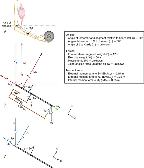
FIGURE 4-21. Problem 2. A, An isometric elbow flexion exercise is performed against an identical weight as that depicted in Figure 4-20. The forearm is held 30 degrees below the horizontal position. B, A free body diagram is shown, including a box with the abbreviations and data required to solve the problem. The vectors are not drawn to scale. C, The joint reaction force (J) vectors are shown in response to the biomechanics depicted in B. The X-Y coordinate reference frame is set so the X direction is parallel to the forearm; black arrowheads point in positive directions.
Figure 4-21, B illustrates the free body diagram of the forearm and hand segment held at 30 degrees below the horizontal (θ). The reference frame is established such that the X axis is parallel to the forearm-hand segment, positive pointed distally. All forces acting on the system are indicated, and each is resolved into their respective X and Y components. The angle-of-insertion of the elbow flexors to the forearm (α) is 60 degrees. All numeric data and abbreviations are listed in the box associated with Figure 4-21.
Resolving Known Forces into X and Y Components: Magnitudes of external forces are found through the use of trigonometric functions, then directions (+ or −) are applied based on the established X-Y axis reference frame:
Solving for Internal Torque and Muscle Force:


The X component of the muscle force, MX, can be solved as follows:
The negative sign was added to indicate MX is pointed in the −X direction.
Solving for Joint Reaction Force: The joint reaction force (J) and its X and Y components (JY and JX) are shown separately in Figure 4-21, C. (This is done to increase the clarity of the illustration.) The directions of JY and JX are assumed to act generally downward (negative Y) and to the right (positive X), respectively. These are directions that oppose the force of the muscle. The components (JY and JX) of the joint force (J) can be readily determined by using Equations 4.13 A and B, as follows:


As depicted in Figure 4-21, C, JY and JX act in directions that oppose the force of the muscle (M). This reflects the fact that muscle force, by far, is the largest of all the forces acting on the forearm-hand segment. JX being positive indicates that the joint is under compression, whereas JY being negative indicates that the joint is under anterior and superior shear. In other words, if JY did not exist, the forearm would accelerate in an anterior and superior (+Y) direction.


Clinical Questions Related to Problem 2:
1. Assume the forearm (depicted in Figure 4-21) is held 30 degrees above rather than below the horizontal plane.
a. Does the change in forearm angle alter magnitude of the external torque?
b. Can you conclude that is it “easier” to hold the forearm 30 degrees above as compared with below the horizontal plane?
2. In what situation would a large force demand on the muscle be a clinical concern?
3. What would happen if, from the position depicted in Figure 4-21, A, the muscle force suddenly decreased or increased slightly?
Answers to the clinical questions can be found on the Evolve website. 
Problem 3: Although the forearm was not positioned horizontally in Problem 2, all resultant forces were depicted as parallel. Problem 3 is complicated slightly by the forces not being parallel, and the bony lever system being a first-class (versus a third-class) lever (see Chapter 1). Problem 3 analyzes the isometric phase of a standing triceps-strengthening exercise using resistance applied by a cable (Figure 4-22, A). The patient can extend and hold her elbow partially flexed against the cable transmitting 15 pounds of force from the stack of weights. Assuming equilibrium, three unknown variables are once again to be determined using the same steps as before: (1) the internal (muscular-produced) torque, (2) the muscle force, and (3) the joint reaction force at the elbow.
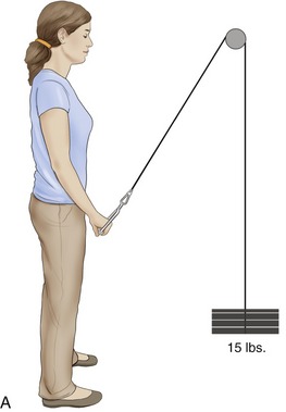
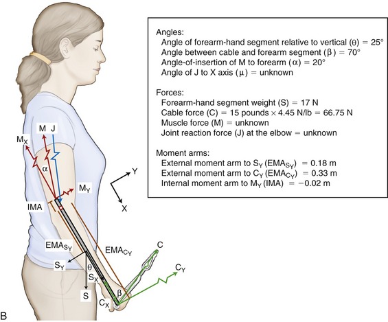
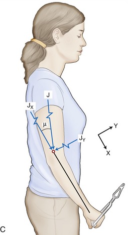
Figure 4-22, B illustrates the free body diagram of the elbow held partially flexed, with the forearm oriented 25 degrees from the vertical (θ). The coordinate reference frame is again established such that the X axis is parallel to the forearm-hand segment, positive pointed distally. All forces acting on the system are indicated, and each is resolved into their respective X and Y components. The angle-of-insertion of the elbow extensors to the forearm (α) is 20 degrees, and the angle between the cable and the long axis of the forearm (β) is 70 degrees. All numeric data and abbreviations are listed in the box associated with Figure 4-22.
Resolving Known Forces into X and Y Components: Magnitudes of forces are found through the use of trigonometric functions, then directions (+ or −) are applied as in previous problems, as follows:
Solving for Internal Torque and Muscle Force: This system is a first-class lever with the muscle force located on the opposite side of the elbow axis as the external forces. The internal moment arm IMA (as applied to MY) is assigned a negative value because the measurement of IMA from the axis of rotation to MY travels in a negative X direction (review no. 5 in Box 4-1).


The X component of the muscle force, MX, can be solved as follows:
The negative sign was added to indicate MX is pointed in the −X direction.
Solving for Joint Reaction Force: The joint reaction force (J) and its X and Y components (JY and JX) are shown separately in Figure 4-22, C. (This is done to increase the clarity of the illustration.) The directions of JY and JX are assumed to act in −Y and +X directions, respectively. These directions oppose the Y and X components of the muscle force. This assumption can be verified by determining the JY and JX components using Equations 4.13 A and B.


As depicted in Figure 4-22, C, JY and JX act in directions that oppose the force of the muscle. JX being positive indicates that the joint is under compression, whereas JY being negative indicates that the joint is experiencing anterior shear. In other words, if JY did not exist, the forearm would accelerate in a general anterior (+Y) direction.
The magnitude of the resultant joint force (J) can be determined using the Pythagorean theorem:

Clinical Questions Related to Problem 3:
1. Figure 4-22 shows the pulley used by the resistance cable located at eye level. Assuming the subject maintains the same position of her upper extremity, what would happen to the required muscle force and components of the joint reaction force if the pulley was relocated at:
2. How would the exercise change if the pulley was located at floor level with the patient facing away from the pulley?
3. Note in Figure 4-22 that the angle (β) between the force in the cable (C) and the forearm is 70 degrees.
Answers to the clinical questions can be found on the Evolve website. 
Dynamic Analysis
Static analysis is the most basic approach to kinetic analysis of human movement. This form of analysis is used to evaluate forces and torques on a body when there are little or no significant linear or angular accelerations. External forces that act against a body at rest can be measured directly by various instruments, such as force transducers (shown in Figure 4-19), cable tensiometers, and force plates. Forces acting internal to the body are usually measured indirectly by knowledge of external torques and internal moment arms. This approach was highlighted in the previous three sample problems. In contrast, when linear or angular accelerations occur, a dynamic analysis must be undertaken. Walking is an example of a dynamic movement caused by unbalanced forces acting on the body; body segments are constantly speeding up or slowing down, and the body is in a continual state of losing and regaining balance with each step. A dynamic analysis therefore is required to calculate the forces and torques produced by or on the body during walking.
Solving for forces and torques under dynamic conditions requires knowledge of mass, mass moments of inertia, and linear and angular accelerations (for 2D dynamic analysis, see Equations 4.15 and 4.16). Anthropometric data provide the inertial characteristics of body segments (mass, mass moment of inertia), as well as the lengths of body segments and location of axis of rotation at joints. Kinematic data, such as displacement, velocity, and acceleration of segments, are measured through various laboratory techniques, which are described next.2,18,20,22 This is followed by a description of the techniques commonly used to directly measure external forces, which may be used in static or dynamic analysis.


KINEMATIC MEASUREMENT SYSTEMS
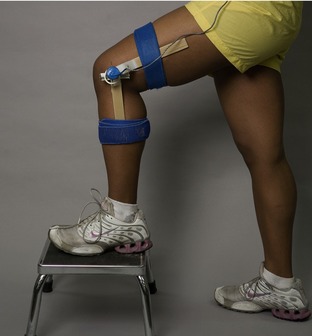
Electrogoniometer: An electrogoniometer measures joint angular rotation during movement. The device typically consists of an electrical potentiometer built into the pivot point (hinge) of two rigid arms. Rotation of a calibrated potentiometer measures the angular position of the joint. The related output voltage is typically measured by a computer data acquisition system. The arms of the electrogoniometer are strapped to the body segments, such that the axis of rotation of the goniometer is approximately aligned with the joint’s axis of rotation (Figure 4-23). The position data obtained from the electrogoniometer combined with the time data can be mathematically converted to angular velocity and acceleration. Although the electrogoniometer provides a fairly inexpensive and direct means of capturing joint angular displacement, it encumbers the subject and is difficult to fit and secure over fatty and muscle tissues. In addition, a uniaxial electrogoniometer is limited to measuring range of motion in one plane. As shown in Figure 4-23, the uniaxial electrogoniometer can measure knee flexion and extension but is unable to detect the subtle but important rotation that also can occur in the horizontal plane. Other types of electrogoniometers exist. Figure 4-24 shows a different style that measures motion in two planes with sensors held onto the subject’s skin by double-sided tape.

Accelerometer: An accelerometer is a device that measures acceleration of the object to which it is attached—either an individual segment or the whole body. Linear and angular accelerometers exist but measure accelerations only along a specific line or around a specific axis. Similar to electrogoniometers, multiple accelerometers are required for 3D or multi-segmental analyses. Data from accelerometers are used with body segment inertial information such as mass and mass moment of inertia to estimate net internal forces (F = m × a) and torques (T = I × α). Whole-body accelerometers can be used to estimate an individual’s relative physical activity during daily life.5,6,9
Imaging Techniques: Imaging techniques are the most widely used methods for collecting data on human motion. Many different types of imaging systems are available. This discussion is limited to the systems listed in the box.
Photography is one of the oldest techniques for obtaining kinematic data. With the camera shutter held open, light from a flashing strobe can be used to track the location of reflective markers worn on the skin of a moving subject (see example in Chapter 15 and Figure 15-3). If the frequency of the strobe light is known, displacement data can be converted to velocity and acceleration data. In addition to using a strobe as an interrupted light source, a camera can use a constant light source and take multiple film or digital exposures of a moving event.
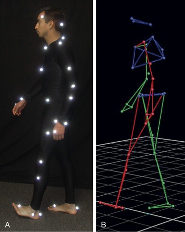
For the most part, still photography and cinematography analysis are rarely used today for the study of human motion. The methods are not practical because of the substantial time required for manually analyzing the data. Digital videography has replaced these systems and is one of the most popular methods for collecting kinematic information in both clinical and laboratory settings. The system typically consists of one or more digital video cameras, a signal processing device, a calibration device, and a computer. The procedures involved in video-based systems typically require markers to be attached to a subject at selected anatomic landmarks. Markers are considered passive if they are not connected to another electronic device or power source. Passive markers serve as a light source by reflecting the light back to the camera (Figure 4-25, A). Two-dimensional and 3D coordinates of markers are identified in space by a computer and are then used to reconstruct the image (or stick figure) for subsequent kinematic analysis (see Figure 4-25, B).
Electromagnetic Tracking Devices: Electromagnetic tracking devices measure six degrees of freedom (three rotational and three translational), providing position and orientation data during both static and dynamic activities. Small sensors are secured to the skin overlying anatomic landmarks. Position and orientation data from the sensors located within a specified operating range of the transmitter are sent to the data capture system.
KINETIC MEASUREMENT SYSTEMS
Mechanical Devices: Mechanical devices measure an applied force by the amount of strain of a deformable material. Through purely mechanical means, the strain in the material causes the movement of a dial. The numeric values associated with the dial are calibrated to a known force. Some of the most common mechanical devices for measuring force include a bathroom scale, a grip strength dynamometer, and a hand-held dynamometer (as shown in Figure 4-19).
Transducers: Various types of transducers have been developed and widely used to measure force. Among these are strain gauges and piezoelectric, piezoresistive, and capacitance transducers. Essentially these transducers operate on the principle that an applied force deforms the transducer, resulting in a change in voltage in a known manner. Output from the transducer is converted to meaningful measures through a calibration process.
One of the most common transducers for collecting kinetic data while a subject is walking, stepping, or running is the force plate. Force plates use piezoelectric quartz or strain-gauge transducers that are sensitive to load in three orthogonal directions (an example of a force plate is shown in Figure 4-27, ahead, under the subject’s forward right foot). The force plate measures the ground reaction forces in vertical, medial-lateral, and anterior-posterior components. The ground reaction force data are used in subsequent dynamic analysis.
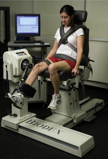
Electromechanical Devices: A common electromechanical device used for dynamic strength assessment is the isokinetic dynamometer. During isokinetic testing, the device maintains a constant angular velocity of the tested limb while measuring the external torque applied to resist the subject’s produced internal torque. The isokinetic system can often be adjusted to measure the torque produced by most major muscle groups of the body. Most isokinetic dynamometers can measure kinetic data produced by concentric, isometric, and eccentric activation of muscles. The angular velocity is determined by the user, varying between 0 degrees/sec (isometric) and 500 degrees/sec during concentric activations. Figure 4-26 shows a person who is exerting maximal-effort knee extension torque through a concentric contraction of the right knee extensor musculature. Isokinetic dynamometry provides an objective record of muscular kinetic data, produced during different types of muscle activation at multiple test velocities. The system also provides immediate feedback of kinetic data, which may serve as a source of biofeedback during training or rehabilitation.
SPECIAL FOCUS 4-7  Introduction to the Inverse Dynamic Approach for Solving for Internal Forces and Torques
Measuring joint reaction forces and muscle-produced net torques during dynamic conditions is often performed indirectly using a technique called the inverse dynamic approach.22 A direct dynamic approach determines accelerations and external forces and torques through knowledge of internal forces and torques. Conversely, an inverse dynamic approach determines internal forces and torques through knowledge of accelerations and external forces and torques. The inverse dynamic approach relies on data from anthropometry, kinematics, and external forces, such as gravity and contact forces. Accelerations are determined employing the first and second derivatives of position-time data to yield velocity-time and acceleration-time data, respectively. The importance of acquiring accurate position data is a prerequisite to the soundness of this approach, because errors in measuring position data magnify errors in velocity and acceleration.
In the inverse dynamics approach, the system under consideration is often defined as a series of link segments. Figure 4-27, A illustrates the experimental setup for investigating the forces and torques in the right lower limb during different versions of a forward lunge exercise with three different trunk and upper extremity positions.5 To simplify calculations, the subject’s right lower limb is considered a linked segment model consisting of solid foot, leg, and thigh segments linked by frictionless hinges at the ankle and knee, and to the body at the hip (see Figure 4-27, B). The center of mass (CM) is located for each segment. In Figure 4-27, C the modeled segments of the right lower limb are disarticulated and the individual forces and torques (moments) are identified at each segment end point. The analysis on the series of links usually begins with the analysis of the most distal segment, in this case the foot. Information gathered through motion analysis techniques, typically camera based, serves as input data for the dynamic equations of motion (Equations 4-15 and 4-16). This information includes the position and orientation of the segments in space and the acceleration of the segments and the segments’ centers of mass. The ground reaction forces (components GY and GX) acting on the distal end of the segment are measured in this example by a force plate built into the floor. From these data the ankle joint reaction force (components JAY and JAX) and the net muscle torque (moments) at the ankle joint are determined. This information is then used as input for continued analysis of the next most proximal segment, the leg. Analysis takes place until all segments or links in the model are studied. Several assumptions made during the use of the inverse dynamic approach are included in the box.
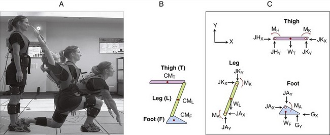
SUMMARY
• Changing the moment of inertia of an arm by bending or straightening the elbow changes the required torque to move the shoulder.
• During an exercise the forces generated by muscles are often many times greater than the external forces used as resistance. This must be considered when a damaged muscle or tendon is being exercised.
• External torque is minimal when the line of force of the external force passes through or near the axis of motion.
• External torque is maximal when the line of force of the external force is at right angles to the limb. When gravity is used as a resistance force, this occurs when the limb is in a horizontal position.
• Internal torque produced by a muscle is maximal when its angle-of-insertion is 90 degrees.
• Exercises are often optimized when external and internal torques are matched through a range of motion.
• Forces at a joint occur as a necessary reaction to the combination of internal and external forces. Muscle force often plays the dominant role in the creation of these joint reaction forces.
Three quantitative-based sample problems were highlighted in this chapter. Two additional problems are available in Appendix I, Part B.
Additional Clinical Connections
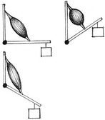
CLINICAL CONNECTION 4-1 A Practical Method for Estimating Relative Torque Potential Based on Leverage
Earlier in this chapter, Figures 4-15 and 4-16 showed two methods for estimating internal and external torques. In both figures, Method 2 is considered a “shortcut” method because the resolution of the resultant forces into their component forces is unnecessary. Consider first internal torque (see Figure 4-15). The internal moment arm (depicted as IMAM)—or leverage—of most muscles in the body can be qualitatively assessed by simply visualizing the shortest distance between a given whole muscle’s line of force and the associated joint’s axis of rotation. This experience can be practiced with the aid of a skeletal model and a piece of string that represents the resultant muscle’s line of force (Figure 4-28). As apparent in the figure, the internal moment arm (shown in brown) is greater in position A than in position B; this means that for the same biceps force, more internal torque will be generated in position A than in position B. In general, the internal moment arm of any muscle is greatest when the angle-of-insertion of the muscle is 90 degrees to the bone.
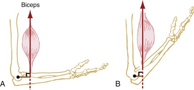
Next, consider the shortcut method for determining external torque. Clinically, it is often necessary to quickly compare the relative external torque generated by gravity or other external forces applied to a joint. Consider, for example, the external torque at the knee during two squat postures (Figure 4-29). By visualizing the external moment arm between the knee joint axis of rotation and the line of gravity from body weight, it can be readily concluded that the external torque is greater in a deep squat (A) compared with a partial squat (B). The ability to judge the relative demand placed on the muscles because of the external torque is useful in terms of protecting a joint that is painful or otherwise abnormal. For instance, a person with arthritic pain between the patella and femur is often advised to limit activities that involve lowering and rising from a deep squat position. This activity places large demands on the quadriceps muscle, which increases the compressive forces on the joint surfaces.
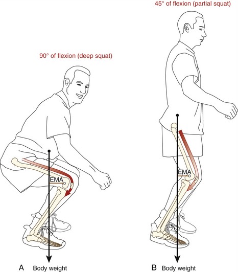
CLINICAL CONNECTION 4-2 Modifying Internal Torque as a Means to Provide “Joint Protection”
Minimizing large muscular-based joint forces may be important for persons with a prosthesis (artificial joint replacement). A person with a hip replacement, for example, is often advised on ways to minimize unnecessarily large forces produced by the hip abductor muscles.12,14,15 Figure 4-30 depicts a simple schematic representation of the pelvis and femur while a person with a prosthetic hip is in the single-limb support phase of gait. In order for equilibrium to be maintained within the frontal plane, the internal (counterclockwise, +Z) and the external (clockwise, −Z) torques around the stance hip must be balanced. As shown in both the anatomic (A) and see-saw (B) illustrations of Figure 4-30, the product of the body weight (W) times its moment arm D1, must be equal in magnitude and opposite in direction to the hip abductor muscle force (M) times its moment arm (D): W × D1 = M × D. Note that the external moment arm around the hip is almost twice the length of the internal moment arm.16,17 This disparity in moment arm lengths requires that the muscle force be almost twice the force of superincumbent body weight in order to maintain equilibrium. In theory, reducing excessive body weight, carrying lighter loads, or carrying loads in certain fashions can decrease the external force and/or the external moment arm and therefore decrease the external torque about the hip. Reduction of large external torques substantially decreases large force demands from the hip abductors, thereby decreasing joint reaction forces on the prosthetic hip joint.
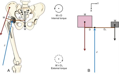
Certain orthopedic procedures illustrate how concepts of joint protection are used in rehabilitation practice. Consider the case of severe hip osteoarthritis, which results in destruction of the femoral head and a subsequent reduced size of the femoral neck and head. The bony loss shortens the internal moment arm length (D in Figure 4-30, A) available to the hip abductor muscles (M); thus, greater muscle forces are needed to maintain frontal plane equilibrium, and greater joint reaction forces result. A surgical procedure that attempts to reduce joint forces on the hip entails the relocation of the greater trochanter to a more lateral position. This procedure increases the length of the internal moment arm of the hip abductor muscles. An increase in the internal moment arm reduces the force required by the abductor muscles to generate a given torque during the single-limb support phase of gait.
CLINICAL CONNECTION 4-3 The Influence of Antagonist Muscle Coactivation on the Clinical Measurement of Torque
When muscle strength is measured, care must be taken to encourage activation of the agonist muscles and relative relaxation of the antagonist muscles (review definitions of agonist and antagonist muscles in Chapter 1). Coactivation of antagonist muscles alters the net internal torque and decreases the ability to control or overcome external forces and torques. This concept is shown with the use of a hand-held dynamometer, similar to that previously described in Figure 4-19. Figure 4-31, A shows the measurement of elbow extension torque with activation only from the agonist (elbow extensor) muscles while the antagonist elbow flexors are relaxed. In contrast, Figure 4-31, B show a maximal-effort strength test of the elbow extensors with coactivation of both the agonist (E) and antagonist elbow flexor (F) muscles. (This situation may occur in a healthy person who is simply unable to relax the antagonist muscles or in a patient with neurologic pathology such as Parkinson’s disease or cerebral palsy.) The internal torque produced by the antagonist muscles actually subtracts from the internal torque produced by the agonist muscles. As a result, the net internal torque is reduced, as indicated by the reduced external force (R) applied against the dynamometer. Because the test condition is isometric, the measured external torque is equal in magnitude but opposite in direction to the reduced net internal torque. The important clinical point here is that even though the elbow extensor forces and torques may be equivalent in tests A and B of Figure 4-31, the external torque measures less in B. This scenario may give an erroneous impression of relative weakness of the agonist muscles when, in fact, they are not weak. As always, the joint reaction force (J) occurs in response to the sum of all forces across the joint and therefore will be increased in test B with antagonist activation.
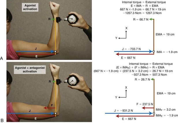
FIGURE 4-31. The influence of coactivation of the agonist (elbow extensor) and antagonist (elbow flexor) muscle groups is shown on the apparent strength (torque) of isometric elbow extension. A, Agonist (elbow extensor) activation only, with the same conditions and abbreviations used in Figure 4-19, A. B, Subject is simultaneously coactivating her elbow extensors and (antagonistic) elbow flexors muscles, producing a simultaneous elbow extension force (E) and an elbow flexion force (F). Because F and E generate oppositely directed torques around the elbow, the net elbow extension torque is reduced. Note, however, that the magnitude of the joint reaction force (J) is increased in B. Vectors are drawn to approximate scale. Based on conventions summarized in Box 4-1, the internal moment arm used by the extensor muscles is assigned a negative number. This, in turn, assigns opposite rotational directions to the opposing internal torques. EMA, external moment arm; IMAF and IMAE, internal moment arms of the elbow flexors and extensor muscles, respectively; R, external force measured by the dynamometer.
REFERENCES
1. Ajemian, S, Thon, D, Clare, P, et al. Cane-assisted gait biomechanics and electromyography after total hip arthroplasty. Arch Phys Med Rehabil. 2004;85:1966–1971.
2. Allard, P, Stokes, IAF, Blanchi, JP. Three-dimensional analysis of human movement. Champaign: Human Kinetics; 1995.
3. Dempster, WT. Space Requirements for the seated operator, WADC-TR-55-159. Dayton: Wright Patterson Air Force Base; 1955.
4. Enoka, RM. Neuromechanical basis of kinesiology, ed 2. Champaign: Human Kinetics; 1994.
5. Farrokhi, S, Pollard, CD, Souza, RB, et al. Trunk position influences the kinematics, kinetics, and muscle activity of the lead lower extremity during the forward lunge exercise. J Orthop Sports Phys Ther. 2008;38:403–409.
6. Hale, LA, Pal, J, Becker, I. Measuring free-living physical activity in adults with and without neurologic dysfunction with a triaxial accelerometer. Arch Phys Med Rehabil. 2008;89:1765–1771.
7. Hamill, J, Knutzen, KM. Biomechanical basis of human movement, ed 3. Philadelphia: Lippincott Williams & Wilkins; 2008.
8. Hatze, H. A mathematical model for the computational determination of parameter values of anthropomorphic segments. J Biomech. 1980;13:833–843.
9. Lee, Y, Lee, M. Development of an integrated module using a wireless accelerometer and ECG sensor to monitor activities of daily living. Telemed J E-Health. 2008;14:580–586.
10. McGibbon, CA, Krebs, DE, Mann, RW. In vivo hip pressures during cane and load-carrying gait. Arthritis Care Res. 1997;10:300–307.
11. Mulroy, SJ, Lassen, KD, Chambers, SH, Perry, J. The ability of male and female clinicians to effectively test knee extension strength using manual muscle testing. J Orthop Sports Phys Ther. 1997;26:192–199.
12. Münger, P, Röder, C, Ackermann-Liebrich, U, Busato, A. Patient-related risk factors leading to aseptic stem loosening in total hip arthroplasty: a case-control study of 5035 patients. Acta Orthop. 2006;77:567–574.
13. Neumann, DA. Hip abductor muscle activity as subjects with hip prostheses walk with different methods of using a cane. Phys Ther. 1998;78:490–501.
14. Neumann, DA. An electromyographic study of the hip abductor muscles as subjects with a hip prosthesis walked with different methods of using a cane and carrying a load. Phys Ther. 1999;79:1163–1173.
15. Neumann, DA. Biomechanical analysis of selected principles of hip joint protection. Arthritis Care Res. 1989;2:146–155.
16. Neumann, DA, Soderberg, GL, Cook, TM. Comparison of maximal isometric hip abductor muscle torques between hip sides. Phys Ther. 1988;68:496–502.
17. Olson, VL, Smidt, GL, Johnston, RC. The maximum torque generated by the eccentric, isometric, and concentric contractions of the hip abductor muscles. Phys Ther. 1972;52:149–158.
18. Özkaya, N, Nordin, M. Fundamentals of biomechanics: equilibrium, motion and deformation. New York: Springer-Verlag; 1999.
19. Simoneau, GG, Bereda, SM, Sobush, DC, Starsky, AJ. Biomechanics of elastic resistance in therapeutic exercise programs. J Orthop Sports Phys Ther. 2001;31:16–24.
20. Soderberg, GL. Kinesiology: application to pathological motion, ed 2. Baltimore: Williams & Wilkins; 1997.
21. Thomas, M, Muller, T, Busse, MW. Quantification of tension in Thera-Band and Cando tubing at different strains and starting lengths. J Sports Med Phys Fitness. 2005;45:188–198.
22. Winter, DA. Biomechanics and motor control of human movement, Hoboken. NJ: John Wiley & Sons; 2005.
23. Zatsiorsky, VM, Seluyanov, V. Estimation of the mass and inertia characteristics of the human body by means of the best predictive regression equations. In: Winter DA, Norman RW, Wells RP, eds. Biomechanics. Champaign: Human Kinetics, 1985.
STUDY QUESTIONS
1. The first set of questions expands on the concepts introduced in Special Focus 4-6. In Figure 4-17, A, assume a constant 50% maximum effort:
a. Describe why internal torque would likely be reduced if the elbow were positioned in 110 degrees of flexion.
b. How does the external torque from gravity acting on the forearm-and-hand segment change if the elbow were to be positioned in 45 degrees of flexion?
2. The next set of questions expands on the concept of muscle coactivation introduced in Clinical Connection 4-3. Using Figure 4-31, B, what would happen to the magnitude of the external force (R) if:
a. F remained the same, but E increased?
b. F remained the same, but E decreased?
3. How does an object’s mass differ from its mass moment of inertia?
a. Provide an example of how the mass moment of inertia of a rotating limb could increase without an increase in its mass.
b. Describe a situation in which the mass moment of inertia of a rotating limb does not affect the force demands of the activated muscles.
4. Where is the approximate location of the center of mass of the human body in the anatomic position?
a. How would the location of the center of mass of the human body change if the arms were raised overhead?
b. How would the location of the center of mass of the human body change after a bilateral (transfemoral) amputation of the legs?
5. In which situation would a muscle produce a force across a joint that does not create a torque?
6. Figure 4-29 shows two levels of external (knee flexion) torque produced by body weight. At what knee angle would the external torque at the knee:
7. Severe arthritis of the hip can cause a bony remodeling of the femoral head and neck. In some cases, this remodeling reduces the internal moment arm of the hip abductors (D in Figure 4-30).
a. In theory, while frontal plane rotary equilibrium around the right (stance) hip is maintained, how would a 50% reduction in internal moment arm affect the hip joint reaction force?
b. Assuming erosion of the articular surface of the femoral head, how would the reduction in internal moment arm affect the hip joint pressure?
8. Assume a person is preparing to quickly flex his hip while in a side-lying (essentially gravity-eliminated) position. What effect would keeping his knee extended have on the force requirements of the hip flexor muscles?
9. Assume the quadriceps muscle shown in Figure 4-18, A has an internal moment arm of 5 cm.
a. Based on the magnitude of the applied external torque, how much knee extensor muscle force is required to maintain static rotary equilibrium about the knee?
b. How much muscle force would be needed if the same external force (100 N) were applied 30 cm distal to the knee?
10. Assume a therapist is helping a patient with weak quadriceps stand up from a seated position from a standard chair. In preparation for this activity, the therapist often instructs the patient to bend as far forward from the hips as safely possible. How does this preparatory action likely increase the success of (or at least ease) the sit-to-stand activity?
 Answers to the study questions can be found on the Evolve website.