Physics

Ultrasonic waves in soft tissues are longitudinal waves that have several physical parameters: frequency (f, in Hz), wavelength (λ, in m), amplitude (u₀, in m), and velocity (c, in m/s).¹ The relationship between velocity, wavelength, and frequency is expressed by the formula: c = λf. Although the velocity of ultrasound is relatively constant in various soft tissues, it is principally dependent on the density (ρ, in kg/m³), stiffness (K, in kg m^–1 s^–2), and temperature of that particular tissue. Another important concept is the (acoustic) impedance (Z, in rayls or kg m^–2 s^–1), which is related to velocity and density as follows: Z = ρc.

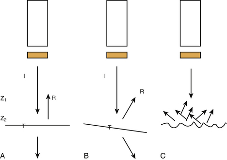
At the boundaries of two types of tissue (or media) a part of the ultrasound is transmitted and another part creates echoes by reflection (Fig. 2.1). These boundaries are called interfaces. The degree of reflection (or intensity reflection coefficient, R) at the interface depends on the impedances of the two media involved. When the ultrasound beam is perpendicular to a smooth interface, R = (Z₂ – Z₁)² / (Z₁ + Z₂)², where Z₁ is the impedance of medium 1 and Z₂ the impedance of medium 2 (see Fig. 2.1A). Therefore, the greater the difference in impedance between two media, the more reflection (or echo) occurs. When the ultrasound beam is not perpendicular to the interface, R and the intensity of the transmitted (refracted) beam are also dependent on the angle of insonation (see Fig. 2.1B). The angle of insonation is measured perpendicular to the interface. The energy is reflected in different directions (scattering) when the ultrasound beam hits a rough surface or small particles (see Fig. 2.1C). During its passage through the various tissues, part of the ultrasound energy is transformed into heat, a process called absorption. As a result of reflection, refraction, scattering, and absorption, the energy of the ultrasound beam is attenuated. Both scattering and absorption are dependent on the type of tissue and the insonation frequency: the higher the frequency the more scattering and absorption. High-frequency ultrasound is therefore less capable of penetrating more deeply located tissues. Reflections from deeper tissues are weaker than those of more superficial structures, and therefore these are usually amplified by time gain compensation.

Fig. 2.1 Reflection, transmission, and refraction of ultrasound at an interface. Perpendicular (A), nonperpendicular (B), and rough surface (C). I, Insonated beam; R, reflected beam; T, transmitted or refracted beam; Z1, impedance of medium 1; Z2, impedance of medium 2.

Transducers

Dependent on the application, one may choose different types of transducers. So-called linear array transducers are used for nerve imaging. These transducers are composed of a row of many single transducers (piezoelectric chemical or crystal elements). The vertical picture lines on the monitor are formed by successive activation of these crystals (the ultrasound beam runs along the array). In modern transducers, a group of neighboring crystals create a single beam that runs along the array by repeatedly moving the group, one element at the time. Transducers produce ultrasound in pulses. These pulses are waveforms with a certain length and can be anatomized into several sinusoidal waves of different frequencies (Fourier analysis). The spectrum of frequencies of these sinusoidal waves is called bandwidth. As the pulse length decreases, the bandwidth increases. Bandwidth and central frequency are both used when referring to the frequency of a transducer. The rate at which the vertical scan lines are activated again is dependent on the pulse repetition frequency (PRF) and the number of scan lines as follows: scan or frame rate equals PRF divided by the number of scan lines. The shape of the ultrasound beam produced by the transducer is like that of an hourglass. The neck represents the focal zone, and there the intensity of the beam is at its maximum. This narrowing of the ultrasound beam is achieved by focusing.

Resolution

The ultimate image quality is dependent on spatial and contrast resolution. Contrast or tissue resolution is defined as the ability to distinguish between different normal tissues and normal from abnormal tissues, whereas spatial resolution refers to the ability to depict and distinguish small objects that are in close proximity.² Spatial resolution can be further divided into axial and lateral resolution. Axial resolution is defined as the ability to separate two objects lying in tandem along the axis of the ultrasound beam. The axial resolution is improved when the pulse length decreases (bandwidth increases) and the insonation frequency increases. The lateral resolution is improved by using a smaller beam width at the focus zone, or by reduction of the frame rate, but also by the technique of successive grouping of crystals as described above. Resolution can be further increased by using multiple rows of crystals.

The Ultrasound

The ultrasound on the monitor is dependent on the echogenicity of the tissue interfaces being insonated. However, in common parlance, it is not the interface that is indicated by its echogenicity, but rather the tissue of interest. One may discern hyperechoic, hypoechoic, and anechoic interfaces. The interface between bone and soft tissue for example is hyperechoic (white on the monitor) because of the great difference in impedance. Cysts are anechoic and appear as black structures on the monitor. Between these two extremes there are more or less hypoechoic structures (for example muscle fascicles), which are depicted in various tones of gray. Normal peripheral nerves appear as tubular echogenic structures with parallel linear internal echoes on longitudinal scans and as round echogenic structures with a honeycomb appearance on transverse scans.

Artifacts

As a result of the properties of ultrasound, there are several possible artifacts.^1,3–5 One should recognize such artifacts because they are potentially misleading. Several artifacts may also degrade the image quality.

Harmonic Imaging

By generating the image from the second harmonic frequencies returning to the probe instead of the original insonating frequency, the quality of the image improves. Because the harmonic frequencies are generated at a deeper level than the surface, clutter, caused by tissue inhomogeneities, is reduced.⁷

Compound Imaging

In real-time spatial compound imaging the ultrasound is created by repeated, overlapping sequences of frames of different predetermined view angles. This technique improves image quality because scanning from different angles reduces acoustic artifacts (e.g., speckle and clutter). The artifacts are suppressed because these patterns are random (not correlated to each other) and averaged during the repeated sequences of scanning. Multiangle scanning is of benefit during musculoskeletal ultrasonography because anisotropy is reduced and small abnormalities can be better visualized.^7,8 A disadvantage of increasing the frame rate is the greater risk of blurring when the transducer is moved too swiftly. Lin and associates systematically examined the image quality of real-time spatial compound ultrasonography as compared with conventional ultrasonography by means of a blinded review of 118 musculoskeletal images by three experienced ultrasonographers using a five-point rating scale. These investigators found that real-time spatial compound ultrasonography significantly improved the image quality (better definition of soft-tissue planes, reduced speckle and other noise, and improved image detail).⁹

XRES

XRES is an image-processing technique that performs real-time analysis of patterns at the pixel level. It looks at the predominated patterns within groups of pixels and brings them into order. It thereby reduces artifacts and brings margins and borders into greater definition.¹⁰

Extended Field-of-View Ultrasound

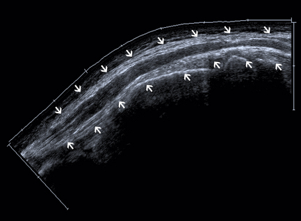
A drawback of using high-insonation frequencies and small (transducer) footprints is the small field of view. A small field of view often makes it difficult or impossible to identify and incorporate landmarks in an image, which are necessary for the orientation of the ultrasound. However, correlating scan frames while moving the transducer will extend the field of view. This technique makes it possible to line up a few consecutive single frames to create a panoramic picture (Fig. 2.2). There are two possible artifacts with the extended field-of-view technique: (1) scanning moving structures may result in distortion, and (2) when the area of interest includes an echo-free area, a skyward deviation of the image may occur because there are no echoes to correlate with when the transducer is moved.¹¹

Fig. 2.2 Panoramic view of the ulnar nerve.

Three-Dimensional Imaging

Three-dimensional (3D) ultrasonography is rapidly gaining popularity as it moves out of the research environment and into the clinical setting, mainly in imaging of breast and abdominal lesions. This modality offers several distinct advantages over conventional ultrasound, including 3D image reconstruction with a single pass of the ultrasound beam; virtually unlimited viewing perspectives; accurate assessment of long-term effects of treatment; and more accurate, repeatable evaluation of anatomic structures and disease entities. However, experience in 3D ultrasonography of peripheral nerves is limited at this time.¹²

Why Is Ultrasonography Suitable for Imaging of Peripheral Nerves?

As a result of the new developments, as described earlier, the resolution of ultrasonography has considerably improved and is even better than that of standard MRI. As many peripheral nerves run a superficial course, they are easily accessible to ultrasonography. Even very small nerves and the fascicular pattern can be studied. The most important artifact during ultrasonography of the peripheral nervous system is anisotropy, which implies that the ultrasonographer must constantly guide the probe to obtain optimum visualization of the nerve. Because of the previously mentioned physical aspects, deeper-lying nerves are more difficult to study. The oblique course of peripheral nerves poses no problems to ultrasonography because the transducer can be moved along the course of the nerve, and extended field-of-view techniques may help create images of peripheral nerves in a longitudinal section over a long segment. This task is hard to accomplish with MRI. Although hyperintensity of nerves on short tau inversion recovery or fat-saturated T2-weighted fast-spin-echo images may indicate disease, this feature is of questionable value because it may also occur as an artifact caused by the magic angle effect.¹³ The echogenicity of a nerve may also be assessed as a marker for disease (e.g., hypoechogenicity may indicate increased water content).

Ultrasonography of peripheral nerves requires the use of transducers with high insonation frequencies (usually 7-12 MHz or more). By increasing the insonation frequency (and decreasing the pulse length) the axial resolution improves. The lateral resolution is improved by using a smaller beam width at the focal zone, by reduction of the frame rate, and by the technique of successive grouping of crystals described earlier. Resolution can be further increased by using multiple rows of crystals. In contrast with conventional ultrasonography, high-resolution ultrasonography is less capable of penetrating into more deeply situated tissues: scattering and absorption are not only dependent on the type of tissue but also on the insonation frequency. Higher frequencies lead to more scattering and absorption. To summarize, small and superficial-lying structures like peripheral nerves may be depicted satisfactorily with high-frequency linear array transducers with multiple rows of crystals.

However, there are a few problems when imaging nerves with ultrasound.

Normal Echogenicity in Healthy Subjects and Cadavers

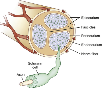
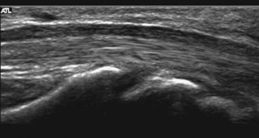
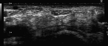
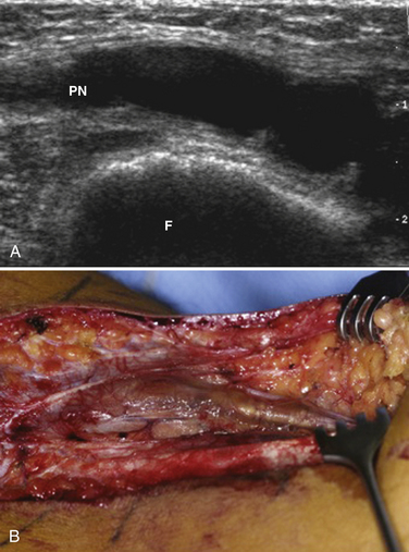
Studies on high-resolution ultrasonography of peripheral nerves date back to the mid-1980s. One of the earliest reports on ultrasonography of peripheral nerves is that of Solbiati and colleagues, who studied the recurrent laryngeal nerve in cadavers and in patients with paralysis of this nerve.¹⁴ Fornage was the first to report systematically on ultrasound of normal peripheral nerves.¹⁵ He studied the median, ulnar, sciatic, and peroneal nerves in cadavers and healthy subjects. The neural fascicle consists of several neural fibers and is embedded in a capsule called perineurium. This capsule consists of connective tissue, vessels, and lymphatic ducts and is thick enough to reflect the sound beam, resulting in hyperechoic lines during high-resolution ultrasound. The trunk of the peripheral nerve consists of several neural fascicles and is embedded in a thicker membrane called epineurium (Fig. 2.3), which is seen as bold echogenic lines with high-resolution ultrasound. Therefore, high-resolution ultrasound of the peripheral nerve is seen as several parallel echogenic lines within two bold echogenic lines in longitudinal section, and as a reticular (honeycomb) pattern in transverse sections. Normal nerves are seen as markedly echogenic tubular structures with parallel internal linear echoes on longitudinal scans (Fig. 2.4) and as oval to round echogenic sections on transverse scans, occasionally with internal punctate echoes (Fig. 2.5).

Fig. 2.3 Normal anatomy of a nerve.

Fig. 2.4 Longitudinal view of the median nerve at the wrist (distal indicates right), showing a tubular structure with parallel internal linear echoes.

Fig. 2.5 Transverse view of the median nerve at the wrist. On transverse view the nerve can have an oval, elliptical, or triangular aspect.

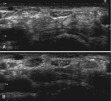
Silvestri and colleagues described the internal structure of cadaver nerves as multiple hypoechoic parallel but discontinuous linear areas separated by hyperechoic bands when scanning in a longitudinal plane, and when scanning transversely as multiple rounded hypoechoic areas in a homogeneous hyperechoic background (fascicular or honeycomb pattern).¹⁶ However, this honeycomb appearance is not always found on transverse sections, and instead the nerve may be more diffusely hypoechoic. They also found that the hypoechoic areas in nerves correlated histologically with fascicles and the hyperechoic background with the epineurium. However, the ultrasounds underestimated the number of fascicles seen during light microscopic examination. The authors suggested that this may be caused by (1) the inability to depict fascicles unless they are perpendicular to the ultrasound beam or (2) poor lateral resolution that results in coalescence of adjacent structures of similar echogenicity.

Differentiating Nerves from Muscles and Tendons

Silvestri and colleagues also paid special attention to the differentiation between nerves and tendons. Tendons appeared to have numerous fine parallel hyperechoic lines separated by fine hypoechoic lines (fibrillar pattern).¹⁶ Fornage used the relative immobility of nerves during flexion-extension maneuvers to differentiate nerves from muscles and tendons.¹⁵ Grechenig and associates found that the perineurium of the sciatic nerve produced bright boundary echoes and variation of the insonation angle reduced echogenicity of the nerve to a lesser extent than that of muscles or tendons.¹⁷

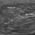
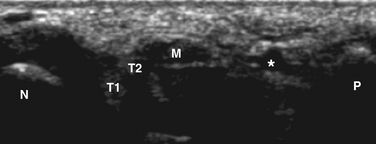
Thus nerves are distinguished from nearby tendons by having less anisotropy (being less variable in echogenicity on variations of the insonation angle) with less fine, tightly packed echoes in parallel (see Video 2.1, Fig. 2.6). The nerve is more immobile and tends to be more oval or eccentric compared with the more circular tendons

Fig. 2.6 Difference between tendon (A) and nerve (B) variation in insonation. Nerves have less variability in echogenicity in comparison with tendons

(see Video 2.1).

Nerve Measurement Techniques

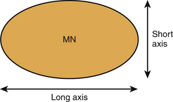
Nerve thickness may be quantified on longitudinal scans by measuring the anteroposterior diameter or on transverse scans by measuring diameters or by calculating the cross-sectional area (Fig. 2.7). Anteroposterior and transverse diameters (D1 and D2) can be measured. The cross-sectional area can be calculated indirectly, assuming an elliptical shape (area = π [D1 x D2]/4), or directly using a continuous boundary trace.

Fig. 2.7 Measuring anterposterior (D1) and transverse (D2) diamaters of a nerve. MN, Median nerve.

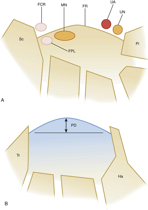
Modern ultrasound machines are usually equipped with software to easily perform these measurements accurately to the tenth of a millimeter. At entrapment sites, such as at the carpal tunnel, flattening of the nerve can be determined as the ratio of the nerve’s major to minor axis. Because maximum nerve enlargement is to be expected at the level of the pisiform bone, a swelling ratio can be calculated by dividing the cross-sectional nerve area at the level of the pisiform bone to the cross-sectional area at the distal radioulnar joint. Another feature of carpal tunnel syndrome is palmar bowing of the flexor retinaculum, which is displacement (measured in mm) of the retinaculum from a line connecting the attachments of this ligament to the tubercle of the trapezium and the hook of the hamate (Fig. 2.8).¹⁸

Fig. 2.8 A, Schematic drawing of the carpal tunnel at the level of the pisiform bone. FCR, Flexor carpi radialis tendon; FPL, flexor pollicis longus tendon; FR, flexor retinaculum; MN, median nerve; Pi, pisiform bone; Sc, scaphoid; UA, ulnar artery; UN, ulnar nerve. B, Schematic drawing of the carpal tunnel at the level of the hook of the hamate. Ha, Hamate; PD, plamar displacement of the flexor retinaculum; Tr, trapezium.

In the literature, several criteria are used to diagnose carpal tunnel syndrome (CTS) by ultrasonography, including:

Fig. 2.9 Normal median nerve at the level of the pisiform bone. M, median nerve; N, Os naviculaire; P, pisiform bone; T1, tendon of the flexor digitorum profundus muscle; T2, tendon of the pollicis longus muscle; ∗, ulnar artery.

(From Visser LH, Smidt MH, and Lee ML: High-resolution sonography versus EMG in the diagnosis of carpal tunnel syndrome, JNNP 79:63–67, 2008.)

Recently ultrasonographic wrist-to-forearm ratio of median nerve cross-sectional area in CTS has also been reported to be a useful test with high sensitivity and specificity,¹⁹ although this was not confirmed by another research group.²⁰ Further discussion of CTS and other focal neuropathies can be found in Chapter 5.

Although many studies do not report whether they include or exclude the hyperechoic rim surrounding the nerve when tracing and making area measurements, most investigators perform measurements erring just to the inside of this rim because it is not always present, and its outer margin may be difficult to define.²¹ During a correlative cadaver study by Kamolz and associates, it was found that ultrasonography was a precise method to assess the dimensions (dorsopalmar diameter, radioulnar diameter, perimeter, and area) of the median nerve at the carpal tunnel.²²

Nerve size depends on the type of nerve and the site of measurement. Relatively large studies to obtain normal values were undertaken by Heinemeyer and Reimers and Cartwright and coworkers.^23,24 Normal values have been obtained for the median and ulnar nerves throughout the entire arm, the radial nerve at the antecubital fossa and spiral groove, musculocutaneous nerve distal to the axilla and between biceps brachii and brachialis muscle, the femoral nerve at the inguinal ligament, the sciatic nerve in the distal thigh, tibial and common peroneal nerves just distal to their bifurcation as well as in the popliteal fossa and dorsal to the fibular head, the peroneal nerve at the fibular head, and the tibial nerve at the ankle and sural nerve in the distal calf (see Table 5.1 for reference values). Maximal nerve thickness is usually measured in sagittal and transverse sections, but the nerve cross-sectional area is the most reliable measurement. In these studies, nerve cross-sectional area correlates with weight, and to a lesser extent with height and body mass index.²⁴

Assessment of Nerve Vascularity by Color Doppler Ultrasonography

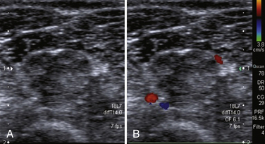
Peripheral nerves are supplied by a rich anastomotic system of epineurial and endoneurial blood vessels (see Fig. 2.3). These two systems are connected via communicating vessels that traverse the perineurium. The homeostasis of the epineurial and endoneurial microenvironment is essential for normal nerve fiber function. Pathologic conditions may give rise to impaired blood supply, substantially contributing to nerve fiber damage in various entrapment and peripheral neuropathies. The effect of altered blood flow has not yet been studied extensively in pathologic conditions. With color Doppler imaging it is possible to detect increased endoneurial or epineurial blood flow²⁵ in CTS, chronic inflammatory demyelinating polyneuropathy (CIDP) (Fig. 2.10), and patients with a type I or type II reaction in leprosy.²⁶ Video 2.2 shows increased endoneurial flow and Video 2.3 presents an example of increased epineurial blood flow. Color Doppler settings are usually chosen to optimize identification of weak signals from vessels with slow velocity. Pulse repetition frequency is set to 1 kHz, and Doppler gain has to be adjusted to the maximum level not producing clutter. Band filter is usually set at 50 Hz. The presence of blood flow signals in the perineural plexus or intrafascicular vessels indicates hypervascularity of the nerve during color Doppler imaging.

Fig. 2.10 Ultrasonography (A) and color Doppler (B) images of an enlarged median nerve in a patient with chronic inflammatory demyelinating polyneuropathy (CIDP), showing increased epineurial flow

(see Videos 2.2 and 2.3).

Edematous (“Swollen”) Nerves

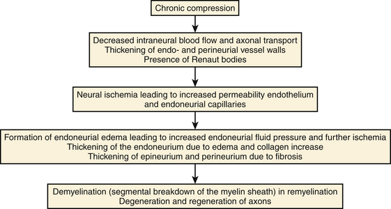
The occurrence of enlarged, hypoechoic nerves is not a disease entity on its own, but a quite common nonspecific reaction of a nerve to various exogenous stimuli. Relative thinning of the nerve occurs at the site of entrapment, whereas enlargement is found more proximally. At an early stage entrapped nerves show thickening of the walls of endoneurial and perineurial microvessels. Later, the endoneurium may become thickened because of edema and an increase in the amount of connective tissue (collagen). In addition, the epineurium and perineurium may thicken because of fibrosis and edema.²⁷

The biologic response to compression is a cascade consisting of endoneurial edema, demyelination, inflammation, distal axonal degeneration, fibrosis, growth of new axons, remyelination, and thickening of the perineurium and endothelium (Fig. 2.11). The development of neural ischemia and endoneurial edema seems to play a role in this process. Normally the endoneurial vessel walls do not allow extravasation of proteins and thereby create a barrier between the blood circulation and the nerve fibers. The perineurial sheath prevents epineurial edema from entering the endoneurial space. However, ischemia caused by compression increases the permeability of the endoneurial vessels, which results in endoneurial edema. This edema cannot be removed because there are no lymph vessels in the endoneurial space and the perineurial membrane forms a diffusion barrier. The result is a progressive increase in endoneurial fluid pressure further obstructing the endoneurial microcirculation and ultimately leading to injury of nerve fibers.²⁷ Possible causes of nerve injury include long-lasting direct compression of a nerve by a plaster cast, metallic implant, or hematoma; stretching of a nerve caused by joint dislocation or during operations; encasement within osseofibrous tunnels; thermal injuries; infection; and blunt trauma. In many cases a nerve with a uniform hypoechoic appearance and thickened fascicles or a sudden change in echo texture at the level of injury is the only apparent ultrasonographic finding.²⁸ In these cases, knowledge about the normal echo structure of an examined nerve is crucial, but interindividual variations may result in misleading findings.

Fig. 2.11 Cascade of pathologic changes in chronic entrapment neuropathy.

Compressive Lesions

Ultrasound may be useful in identifying compressive lesions. Direct compression of a nerve by surrounding tissue may occur by normal anatomic structures such as in nerve entrapment syndromes or by abnormal structures such as vascular malformations, malaligned fractures, ganglia (Fig. 2.12), or tumors. Ganglia may occur in any location adjacent to joints or tendon sheaths. Direct compression of a nerve may also be caused by external compression, posttraumatic hematoma or callus formation as well as postoperative scars.

Fig. 2.12 Intraneural ganglion in the peroneal nerve (PN) at the fibula head (F) by ultrasonography (A) and confirmed at surgery (B).

(From Visser LH: High resolution ultrasonography of the peroneal nerve: detection of intraneural ganglia, Neurology 67:1473–1475, 2006.)

Tumors

The most commonly encountered benign peripheral nerve tumors are neurofibromas and schwannomas, whereas other benign histologic types and malignant peripheral nerve sheath tumors are rare entities.²⁸ Because schwannomas derive from cells representing the supporting tissue of a nerve, they typically appear as ovoid masses arising from the surface of a nerve separated from the unimpaired nerve fascicles. The nerve itself may be stretched over the capsule of the mass. In neurofibromas, tumor cells spread within the nerve fascicles, giving the nerve a spindle-shaped appearance. The fascicular pattern typically disappears at the site of the lesion. Neuromas are masslike nerve lesions not representing true tumors, but rather reactive local thickening of a nerve due to various extrinsic causes such as severe traction injury or dissection of a nerve. In these lesions some or all nerve fascicles are severed with loss of continuity. A special subset of neuromas with distinct pathophysiology exists in the interdigital spaces at the level of the metatarsals. These lesions known as Morton’s neuromas are typically located at the level of the metatarsal heads in the second or third interspace and caused by repeated chronic microtrauma with resulting painful fibrosis of an interdigital nerve.

Hypertrophy of Nerves

Several hereditary polyneuropathies, linked to genes that produce products essential for myelin function, such as PMP22, myelin protein zero and connexin-32, may have nerve thickening as a result of hypertrophic changes comprising onion bulb formation, segmental demyelination and remyelination, lack of large and small myelinated fibers, and an increase in endoneurial edema.²⁹ Further discussion of ultrasonographic changes seen in polyneuropathies can be found in Chapter 7.

Inflammation

Chronic inflammatory demyelinating polyneuropathy results in enlargement of nerves due to remyelination, onion bulb formation, and cellular infiltrates.³⁰ A typical example of neuritis is leprosy. The lepromatous form is characterized by actively proliferating Mycobacterium leprae and minimal inflammatory response, whereas the tuberculoid form shows an intense inflammatory response with few organisms in skin and nerve. Nerves running a subcutaneous course may become palpably thickened, especially in the tuberculoid stage, reflecting the histopathologic changes that take place. In the beginning of the lepromatous form, bacteria invade the Schwann cells. When these cells become overloaded, cell death occurs and other parts of the nerve are invaded, producing segmental demyelination and remyelination, reactive proliferation of endoneurial connective tissue, lesions of the intraneural blood vessels, and perineurial thickening. In tuberculoid leprosy a granulomatous inflammation results in loss of axons, Schwann cells, and myelin. Ultimately, endoneurial and perineurial fibrosis produces nodular nerve thickening. In addition, intraneural vascular lesions are found (see Videos 2.2 and 2.3).³¹

Nerves of the Upper Extremity

Normal Ultrasonographic Anatomy of the Carpal Tunnel and Median Nerve

The carpal tunnel can be divided into a proximal part, at the level of the pisiform bone, and a distal part, at the level of the hook of the hamate. These hypoechoic bony structures serve as landmarks for the quantitative analysis of the median nerve (see Figs. 2.8 and 2.9). The ventral border of the carpal tunnel is formed by the hyperechoic flexor retinaculum, which extends from the pisiform to the scaphoid bone proximally and from the hook of the hamate to the trapezium distally. The retinaculum has a width of 3 to 4 cm and is thickest at the distal carpal tunnel. Lying just beneath the retinaculum, the median nerve has a close relationship to the tendons of the flexor pollicis longus and flexor digitorum superficialis. Ventral to the retinaculum, the ulnar artery (and nerve) can be found at the medial side of the hand.

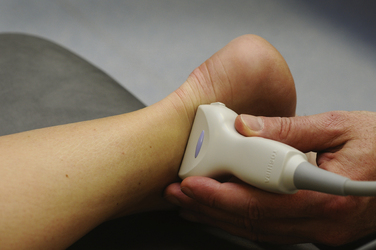
Median Nerve Ultrasound Technique

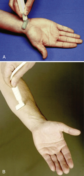
Subjects are seated facing the examiner. The arms are extended, wrists resting on a flat surface, forearms supinated, and fingers extended (Fig. 2.13). When starting ultrasonography of the median nerve, the nerve is most likely to be found by placing the transducer (18-7 MHz) in a transverse orientation, approximately 7 cm proximal to the carpal tunnel, and looking for an echogenic structure with a honeycomb structure. The nerve can then be followed to the proximal carpal tunnel. One has to be careful not to confuse the nerve with the palmaris longus. Transverse images of the median nerve with measurements of the cross-sectional area are usually obtained at two levels: at the carpal tunnel inlet at the distal wrist crease and at the distal one third level of the forearm. The cross-sectional area of the median nerve can be determined by outlining the nerve contour, erring to the internal side of the hyperechoic rim, using area measurement software (continuous boundary trace) of the ultrasound system. All the measurements should be rounded to the nearest 0.01 cm². It is important to keep the ultrasound beam perpendicular to the nerve, especially when measurements are performed. The echogenicity of the nerve may serve as a guide: slight angulation of the beam results in hypoechogenicity (anisotropy) of the tendons, but this is not as pronounced in the nerve. Because the shape of the median nerve in the carpal tunnel may change with different wrist positions, most investigators use a neutral position. A possible cause of artificial nerve deformation is the force with which the transducer compresses the skin surface, but this change is not large. During its course through the carpal tunnel the shape of the median nerves changes. Proximal to the carpal tunnel it is circular on transverse scans. Within the carpal tunnel it is most often described as ovoid, sometimes as flat-elliptical.

Fig. 2.13 Ultrasound technique used to examine the median nerve at the wrist (A) and lower arm (B).

Distally the nerve dives under the flexor retinaculum and becomes more difficult to visualize. The distal carpal tunnel is more difficult to study because the nerve is deeper and oblique to the transducer, and the signal-to-noise ratio is usually poor. If followed carefully, it can be seen to split into multiple small branches, which can be followed up to the digits. As the probe is moved proximally from the wrist, the nerve is seen to wrap around deep to the flexor digitorum superficialis tendons. Once it locates deep to this muscle, it is less flattened and sometimes almost triangular in shape in addition to becoming more echogenic.

Nakamichi and Tachibana found that when the entire course of the median nerve through the carpal tunnel was considered, it may have the configuration of an hourglass (head, neck, body), even in normal subjects. The head is located beneath the distal edge of the flexor retinaculum, the neck at the level of the hook of the hamate (where the retinaculum is thickest), and the body at the wrist crease (proximal to the pisiform bone).³² The nerve can then be tracked proximally up the forearm as it continues to become deeper in location. Distal to the antecubital fossa, it rises closer to the surface to join the brachial artery.

Tendons are easily distinguished from the nerve by simply having them move, actively or passively. In the sagittal plane the proximal-distal movement of the tendons is unmistakable. During voluntary movement of the hands, there is considerable movement of the median nerve apparent in the axial plane. With simple piano-playing motions of the fingers, the tendons are seen to jostle and bump the nerve. If the fingers are fully flexed, followed by wrist flexion, often ending up surrounded by the tendons encompassed by the carpal tunnel.³³

Median Nerve and Underlying Abnormalities

1. Mass lesions. It is well known that ultrasonography can detect soft-tissue masses. Space-occupying lesions such as lipomas, hemangiomas, hematomas, fibromas, and ganglion cysts may cause CTS. Patients with unilateral CTS are more likely to have a space-occupying lesion (most often an occult ganglion cyst).

2. Anatomic variants. Ultrasonographic imaging may demonstrate anatomic variants such as a persistent median artery or bifid median nerve.

3. Rheumatoid arthritis. Bilateral synovial thickening may be the initial manifestation of rheumatoid arthritis.

Normal Ultrasonographic Anatomy of the Ulnar Nerve

The ulnar nerve arises from the medial cord (C8 to T1) of the brachial plexus. The nerve descends medial to the brachial artery, intervening between it and the brachial vein. At the lower third of the arm it pierces the medial intermuscular septum and descends in front of the medial head of the triceps. The ulnar nerve is found easily in the upper third of the arm because of its relation to the ulnar artery, which lies lateral to the nerve. Distally, it extends more medial to enter the cubital tunnel. At the elbow, it lies in a groove on the dorsum of the medial epicondyle. The ulnar nerve descends through the medial side of the forearm, lying deep to the flexor carpi ulnaris muscle, in close relation with the flexor carpi ulnaris tendon, and close to the medial side of the ulnar artery in the lower two thirds.³⁴

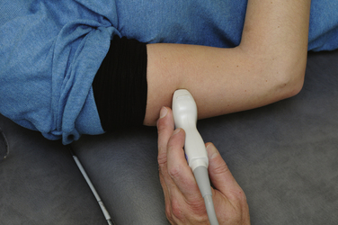
Ulnar Nerve Ultrasound Technique

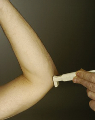
The ultrasound examination can be performed when the patient is either lying or sitting. Our experience is that the examination can be best performed with the patient supine with the forearm above the head and the elbow flexed at 70 degrees (Fig. 2.14). This is a comfortable position for the patient and examiner, but one has to be sure that the patient does not have shoulder pain. The ulnar groove can then easily be accessed. The nerve can most easily be found by placing the probe 5 cm below the elbow, and after detection of the honeycomb structure of the ulnar nerve, the nerve can be followed more proximally into the cubital tunnel. From the cubital tunnel the ulnar nerve can be followed distally to Guyon’s canal and proximally to the axilla. In the case of an ulnar neuropathy at the elbow, we usually measure the height (in longitudinal view) and cross-sectional area at the level of the medial epicondyle and 2 to 3 cm proximal to and 2 to 3 cm distal to this level. Interobserver agreements of the ultrasonographic diameter measurements have shown to be good (intraclass correlation coefficient for continuous measures 0.91).

Fig. 2.14 Ultrasonographic examination of the ulnar nerve at the elbow.

In addition to the diagnostic value in idiopathic ulnar neuropathy, ultrasonography may also detect possible causes of ulnar neuropathy at the elbow, such as an occult ganglion, an anconeus epitrochlearis muscle, a snapping triceps, or an ulnar nerve dislocation.

Normal Ultrasonographic Anatomy of the Radial Nerve

The radial nerve is the largest branch of the brachial plexus formed by axons from C5 to T1 roots. It carries motor fibers, mainly for the extensor muscles of the arm and hand. It also contains cutaneous sensory afferents from the posterior arm, forearm, and hand (Fig. 2.15). Just above the arcade of Frohse in the proximal forearm, the radial nerve branches into the posterior interosseous nerve, that contains only motor fibers, and the superficial radial sensory nerve. In the distal forearm the superficial radial nerve traverses a superficial subcutaneous course, running between the tendons of the brachioradialis and extensor carpi radialis longus and crossing the lateral edge of the radius.

Fig. 2.15 Ultrasonographic examination of the radial nerve at the upper arm.

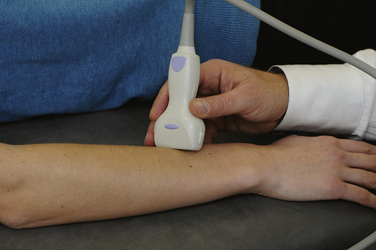
Radial Nerve Ultrasonographic Technique

As for most superficially located nerves, linear array transducers of 18-12 MHz are necessary. The radial nerve is easily traced from the spiral groove of the humerus proximally to an area between the medial and lateral heads of the triceps muscle. For the superficial radial nerve, the examination can be performed with the arms pronated on a table. By scanning transversely, the superficial radial nerve can be seen approximately 9 cm above the level of the distal radius and then followed distally over the dorsolateral aspect of the forearm (Fig. 2.16). Once the nerve is located, it can be followed more proximally to the antecubital fossa or more distally to the wrist.

Fig. 2.16 Ultrasonographic examination of the superficial radial nerve in the forearm.

Nerves of the Lower Extremity

Normal Ultrasonographic Anatomy of the Sciatic, Peroneal, Tibial, and Sural Nerves

The sciatic nerve is the longest peripheral nerve. It leaves the pelvis through the infrapiriform foramen. Proximal to the popliteal fossa it divides into the peroneal and tibial nerves. This division is easily seen by ultrasonography. Within the popliteal fossa the common peroneal nerve follows the medial edge of the biceps muscle to the head of the fibula, where it enters the peroneal compartment.

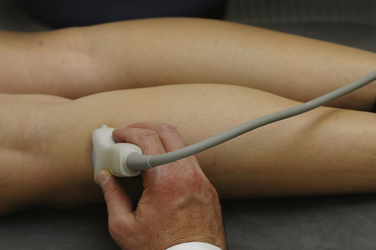
Ultrasound Technique

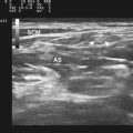
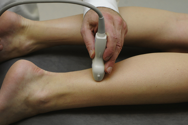
Examination is done with the patient lying prone with extended knees. The sciatic nerve is a large nerve bundle that can be traced from the popliteal fossa transversely, lateral to the popliteal vessels, between the biceps femoris (lateral) and the semimembranous and semitendinous (medial) muscles. From the posterior fossa the division into the peroneal nerve and tibial nerve can be examined. It is also possible to first localize the fibula head and locate the peroneal nerve just proximal from the fibula head (Fig. 2.17). The nerve can be measured at this site and thereafter can be followed proximally. At the popliteal fossa the tibial nerve is adjacent to the popliteal artery and vein (see Video 2.4). In the ankle, the tibial nerve can be easily determined just proximal to the ankle, at the medial site, running adjacent to the flexor digitorum longus tendon and posterior tibial artery and vein (Fig. 2.18).²⁸ The sural nerve can be visualized approximately 8 cm above the ankle, at the distal calf, on either side often bordered by two compressible veins (Fig. 2.19).²⁴

Fig. 2.17 Ultrasonographic examination of the peroneal nerve at the fibula head.

Fig. 2.18 Ultrasonographic examination of the tibial posterior nerve in the ankle.

Fig. 2.19 Ultrasonographic examination of the sural nerve in the calf.