Chapter 3 Ultrasound of Muscle
 Video 3.1:
 Video 3.2:
 Video 3.3:
 Video 3.4:
 Video 3.5:
In 1980 it was discovered that diseased muscles have a different ultrasound appearance compared with healthy muscles.1 Patients with neuromuscular disorders were found to have higher muscle echogenicities, that is, whiter muscles. Beside neuromuscular disorders, malignancies, infections, hematomas, and ruptures of the musculoskeletal system can be detected with ultrasound.2–5 Over time, ultrasound techniques have improved, resulting in the display of muscle tissue with resolutions up to 0.1 mm.6 This is higher than the resolution that can be achieved with 3 Tesla magnetic resonance imaging (MRI), which has a resolution of up to 0.2 × 0.2 × 1 mm.7 Moreover, ultrasound’s dynamic imaging and real-time function make it possible to detect muscle movements and even spontaneous muscle activity such as fasciculations. This chapter provides insight into the technique of quantitative and dynamic muscle ultrasound imaging and an introduction of its use in neuromuscular disorders.
Basics of Ultrasound Physics in Relation to Muscle Ultrasound Imaging
Reflections and Acoustic Impedance
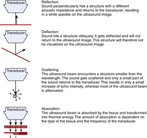
Sound waves and their reflections form the basis of ultrasound images. A transducer sends out pulses of high-frequency sound waves and receives their echoes. Reflection of sound waves can occur when the ultrasound beam encounters a different tissue. Two factors influence the amount of reflection: the acoustic impedance of the two tissues and the angle between the direction of the sound wave and the reflecting surface (Fig. 3.1).8–9
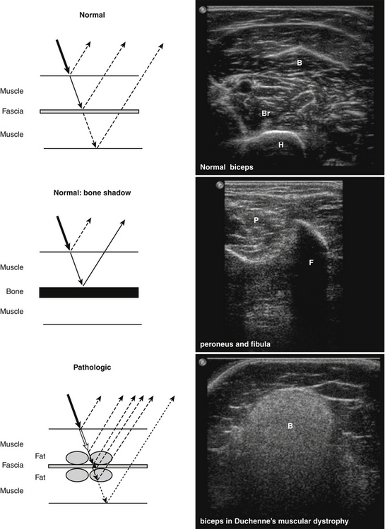
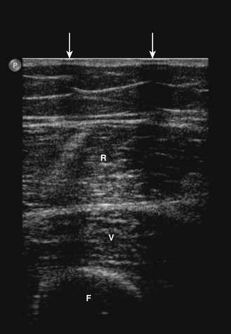
The acoustic impedance is made up by the combination of density of the tissue and the sound velocity within the tissue. The latter is different for each tissue type (Table 3.1). The largest differences in acoustic impedance are found between bone and air, in which sound has a velocity of approximately 300 and 4000 m/s, respectively, whereas in muscle the sound velocity is approximately 1580 m/s.9 The larger the difference in acoustic impedance, the larger the amount of reflection of the ultrasound beam. A small difference in acoustic impedance will result in no reflection or reflection of only a small part of the sound wave, whereas most of the ultrasound beam can pass through to deeper layers. This is also the case in muscle: histologic structures in healthy muscle will mostly transmit sound (Fig. 3.2). Conversely, a transition with a very large difference in acoustic impedance will result in reflection of all sound waves. Beneath such a transition no imaging is possible. For example, the difference in acoustic impedance of air and skin is very large, which makes it impossible to produce ultrasound images without the help of a gel or another contact fluid between the transducer and the skin (Fig. 3.3). A transition from muscle to bone or calcifications will also cause a strong reflection. As the amplitude of the sound wave corresponds to the brightness of the image, the strong reflections of bone result in a bright spot on the ultrasound image. Additionally, because hardly any sound gets through, no structures beneath this transition can be displayed, resulting in a characteristic bone “shadow” (see Fig. 3.2).
| Tissue | Sound Velocity (m/s) |
|---|---|
| Air | 330 |
| Fat | 1450 |
| Water | 1540 |
| Connective tissue | 1540 |
| Blood | 1570 |
| Muscle | 1585 |
| Bone | 4080 |
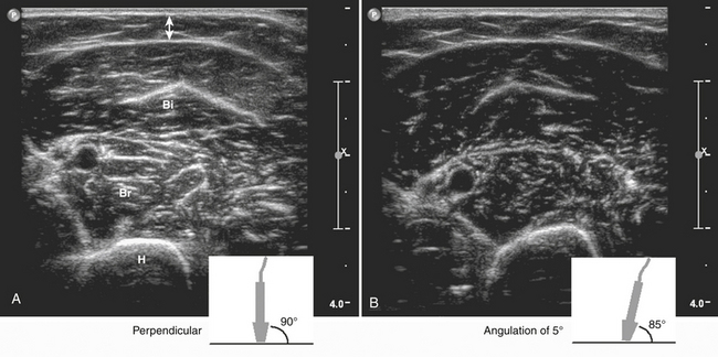
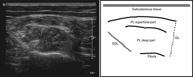
The amount of sound reflection is also determined by the angle at which the ultrasound beam reaches a tissue transition.8–9 A large angle will result in deflection (away from the transducer) instead of reflection of the sound. In this way, the sound wave will not return to the transducer and the structure will not be displayed (see Fig. 3.1). Because of this, fascia surrounding muscle, nerves, and bone will be especially echogenic when they are reached perpendicular by the ultrasound beam. Oblique scanning will cause deflection and diminishes the echogenicity of these structures (Fig. 3.4). Moreover, fascia between muscles that are in line with the ultrasound beam is difficult to visualize; the fascia remains either black or is displayed as an interrupted line (Fig. 3.5).
When the ultrasound beam encounters structures smaller than the wavelength of the sound emitted, such as individual muscle fibers, the sound waves are not reflected but scattered (see Fig. 3.1).9 Only a small part of this sound will return to the transducer, and will therefore result in only a small increase of the gray level in the picture.
Choice of Transducer Frequency
When the sound beam travels to deeper layers, attenuation of the ultrasound beam occurs. Less sound reaches deeper levels, caused by reflection and scattering, but also by absorption and transformation of the beam into thermal energy. The amount of absorption depends on the type of tissue and is, for example, very high in bone. It increases with higher transducer frequencies (Fig. 3.6). For average soft tissues, the loss amounts to approximately 1 dB per 10-mm tissue depth for each MHz. As a rule, the depth penetration is limited to about 200 mm for a 3-MHz probe, 100 mm for a 6-MHz probe, and 12 mm for 50-MHz probe.6
Axial resolution is determined by the transducer frequency. As higher frequencies are accompanied by smaller wavelengths, a transducer with the highest frequency will achieve the best axial resolution. The lateral resolution is best in the focal zone of the ultrasound beam and is several times larger than the axial resolution.6 This means that when the focus of the ultrasound beam is positioned at a depth that contains the structures of interest (i.e., the muscles under investigation) these structures will be visualized with the best lateral resolution.
Normal Muscle
Histology
To understand what is visualized with muscle ultrasound, it is also necessary to know the architecture of muscles up to the maximum resolution of muscle ultrasound. Muscles are composed of individual muscle fibers that normally have a diameter of approximately 40 to 80 μm.10 The resolution of muscle ultrasound is around 100 μm, which means that either one large fiber or a group of small muscle fibers are the smallest structures within muscle that can be visualized. Each muscle fiber is surrounded by thin fibrous tissue called endomysium. A group of muscle fibers forms a muscle fascicle, surrounded by perimysium. This connective tissue also contains small blood vessels and nerves. The outside covering of the muscle is made of fibrous tissue called epimysium, which is thicker and stronger than perimysium (Fig. 3.7). The epimysium continues at the origin and insertion to form tendons and sheetlike tendons called aponeuroses.11
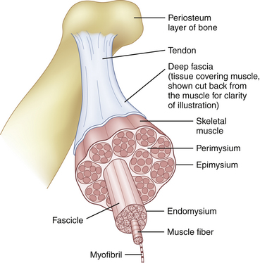
Fig. 3.7 Normal muscle architecture.
(Adapted from The structure of muscle and associated connective tissues. lvyRose Holistic: Holistic Health, Alternative Medicine, Human Biology, and Anatomy & Physiology. Available at www.ivy-rose.co/uk/humanbody/muscles/muscle_structure.php. Accessed June 2008.)
The organization of muscle fascicles results in the macroarchitecture of a muscle. In some muscles, the fibers run parallel to the long axis of the muscle and a few of them run through its whole length (Fig. 3.8A). In other muscles, the fibers are obliquely oriented to the long axis of the muscle. Because of their resemblance to feathers these are called pennate muscles (see Fig. 3.8B). They can be divided in unipennate muscles when the fibers have one linear origin resembling one half of a feather; bipennate muscles when the fibers arise from a broad surface resembling a whole feather; multipennate muscles when septa extend into the attachment of the muscles, dividing them into several feather-like portions; and circumpennate muscles when the fibers converge on a tendon extending into their substance (like the feathers of a dart). In other muscles, the fibers converge from a wide attachment to a fibrous apex (see Fig. 3.8C). This type of muscle is described as a fan-shaped or triangular muscle.12
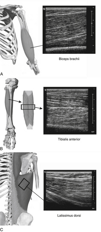
(Part of the anatomical drawings were modified and used with permission from PreventDisease.com: Muscle atlas. Available at www.preventdisease.com/home/muscleatlas.shtml. Accessed June 2008.)
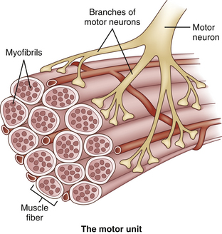
Apart from a structural or histologic organization, muscles also have a functional or physiologic organization. This functional unit is called a motor unit, consisting of one motor neuron and the muscle fibers it controls (Fig. 3.9). The number of muscle fibers in a motor unit varies from less than 10 to several hundred, according to the size and function of the muscle. Large motor units, where one neuron supplies several hundred muscle fibers, are found in the trunk and thigh muscles, whereas motor units of small eye and hand muscles, where precision movements are required, contain only a few muscle fibers. The muscle fibers of a motor unit are not grouped together but spread among the muscle fascicles.11 Therefore, the diameter of a motor unit can range from less than one millimeter to more than one centimeter wide. Because muscle fibers have no anatomic features that attribute them to one particular motor unit, it is impossible to tell with an imaging technique which muscle fibers belong to which motor unit. Hypothetically, if pathology was confined to one motor unit or a single motor unit was activated and would contract, imaging techniques might be able to visualize this particular motor unit provided that the resolution is sufficient.
Ultrasound of Normal Muscle Tissue
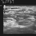
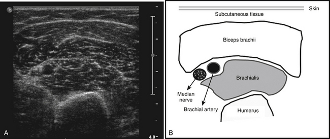
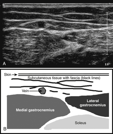
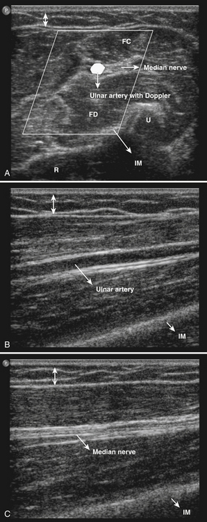
The ultrasonographic appearance of muscles is fairly distinct and can easily be discriminated from surrounding structures such as subcutaneous fat, bone, nerves, and blood vessels (Fig. 3.10).13–14 Normal muscle tissue is relatively black, that is to say, it has a low echogenicity. In the transverse plane, which is perpendicular to the long axis of the muscle, muscle tissue has a speckled appearance because of reflections of perimysial connective tissue that is moderately echogenic (see Fig. 3.10). In the longitudinal plane (parallel to the long axis of the muscle) the fascicular architecture of muscle tissue becomes visible. Reflections of the perimysial connective tissue result in a linear, pennate, or triangular structure on the ultrasound image (see Fig. 3.9). The boundaries of the muscle are clearly visible because the epimysium surrounding the muscle is a highly reflective structure. In normal subjects, the bone echo beneath the muscle is strong and distinct with an anechoic bone shadow underneath (see Fig. 3.2B). Subcutaneous fat has a low echogenicity, but several echogenic septa of connective tissue may be visible within this tissue layer (Fig. 3.11). Nerves and tendons are relatively hyperechoic compared with healthy muscles, whereas blood vessels are hypoechoic or anechoic circles or lines depending on the direction of the ultrasound beam (Fig. 3.12A). When one is unsure about the nature of a round or linear structure, Doppler imaging can confirm the presence of arteries or veins, by showing blood flow (Fig. 3.12B).
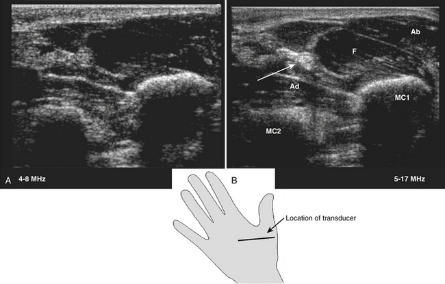
All superficial muscles can easily be imaged with ultrasound, although it can be difficult to identify individual small muscles when multiple muscle groups overlap. Recent ultrasound technology using higher transducer frequencies with corresponding higher axial resolutions has made it possible to image individual superficial small muscles in, for example, the hand (Fig. 3.13). Deeper muscles, especially in the pelvic region or around the trunk, can be difficult to visualize with sufficient resolution because of the reflection or absorption of sound by superficial tissue layers, such as skin, subcutaneous tissue, or other muscles.
Muscle Thickness
Muscle ultrasound is a reliable method to measure muscle thickness and cross-sectional areas,15–17 with a test-retest correlation of 0.98 to 0.9915,18 and a 0.99 correlation MRI.15 Several studies have used ultrasound to establish muscle thickness in healthy subjects. During childhood, muscle thickness increases rapidly. The main variable to predict muscle thickness in this age group is weight.19 Gender differences do not influence muscle thickness until puberty, when men start to develop bigger muscles than women.20–22 After puberty muscle thickness increases further in both genders, until a peak is reached between 25 and 50 years of age. Thereafter, muscle thickness declines.21–24 The influence of age and gender is different for each muscle group and should be taken into consideration when evaluating muscle ultrasound scans of individual patients.
Muscle Echogenicity
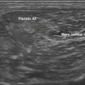
Muscle structure can also be evaluated with ultrasound by evaluating muscle echogenicity. Normal muscles are relatively black, but different muscles have specific appearances on ultrasound because of the variability in proportion of fibrous tissue and the orientation of muscle fibers. For example, the anterior tibial muscle has generally a whiter appearance than the rectus femoris.19
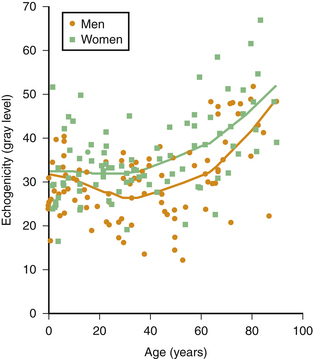
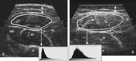
Muscle echogenicity increases with age, which is caused by age-related replacement of muscle fibers by fat and fibrous tissue.25,26 Figure 3.14 shows an example of this age-related increase in muscle echogenicity of the biceps brachii muscle. Fat and fibrous tissue have a different acoustic impedance, increasing the number of reflecting interfaces in the muscle, which gives the muscle a whiter appearance (see Fig. 3.2B). Essentially, the same mechanism also causes increased muscle echogenicity in neuromuscular disorders.1,27 The visibility of structures in and surrounding the muscle can provide additional clues about the presence of structural muscle changes. In several neuromuscular disorders, such as muscular dystrophies and spinal muscular atrophy, this finding can be as prominent as the increase in muscle echogenicity.28,29
Visual detection of slightly increased muscle echogenicity can be difficult and its accurate interpretation depends on the experience of the observer, especially because different muscles have different appearances, and muscle echogenicity increases with age. Changes in ultrasound system settings, such as increased gain, can also give muscles a whiter appearance that can be mistaken for pathologically increased echogenicity. For these reasons, visual evaluation of muscle ultrasound has shown a relatively low interobserver agreement (kappa 0.53) that further deteriorated when an inexperienced observer interpreted the images.30 To overcome this problem, computer-aided techniques were introduced to help image interpretation. Quantification of muscle echogenicity can be achieved with simple gray scale analysis (Fig. 3.15).23,30–32 Quantitative echogenicity analysis is a robust clinical technique with a high interobserver agreement (kappa 0.86).30 It is also suitable for research purposes.
Next to calculation of mean echogenicity, other quantitative techniques such as backscatter analysis have been introduced in muscle ultrasound because this technology is less influenced by system settings.33 This technique compares measured echo intensity with phantom measurements, to make it easier to compare echogenicity measurements made using different ultrasound devices. However, some hardware differences, especially differences in transducers, can still be a problem when using normal values established in other centers. Moreover, this technique has not yet been validated in a large prospective study.
Even with quantitative echogenicity analysis, visual evaluation of the images still has its value. Focal changes in a muscle that has a normal overall muscle echogenicity can easily be detected visually. Visual evaluation also provides information on the distribution of echogenicity within a muscle, that is, whether it is homogeneous or inhomogeneous. New developments in digital image analysis, such as texture analysis, are being designed to quantify these alterations within muscle tissue.25,34 These techniques are already used for detecting focal changes in other tissues, such as the breast and prostate.35–36
Muscle Ultrasound in Neuromuscular Disorders
Neuromuscular disorders usually lead to changes in muscle morphology, and these can be visualized with ultrasound. Both atrophy and changes in muscle architecture can be assessed. The latter is the proved method for measuring echogenicity.37 Studies have shown a strong correlation between the disruption of normal muscle architecture and muscle echogenicity.26,38–39 Both fat and fibrous tissue are responsible for the increased echogenicity.
Prospective studies in children have shown that with visual evaluation of muscle echogenicity, the presence of a neuromuscular disorder can be detected with a sensitivity of only 67% to 81% and a specificity of 84% to 92%.40–42 Quantification of muscle echogenicity improved the sensitivity to 87% to 92%.27,30,32,37 With this high sensitivity, muscle ultrasound is suitable for screening purposes. In adults, prospective studies investigating the diagnostic value of muscle ultrasound are in progress.
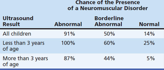
These sensitivities and specificities represent the overall ability of muscle ultrasound to detect neuromuscular disorders. However, in specific neuromuscular disorders or in specific age groups these values differ (Table 3.2). For example, the sensitivity of ultrasound in detecting Duchenne’s muscular dystrophy in clinically affected patients approaches 100%,27 whereas mitochondrial myopathies will only be detected by ultrasound in 25% to 45% of the symptomatic cases.43 In children younger than the age of 3 years, muscle ultrasound has also shown a lower sensitivity (approximately 75%).27,41–42 This is explained by the fact that structural changes within muscle can still be minor in the early stages of a neuromuscular disorder. However, because the specificity of muscle ultrasound for the presence of a neuromuscular disorder is still high in these children (approaching 100%), an abnormal ultrasound has major implications in directing further—more invasive—investigations.
Table 3.2 Chance of the Presence of a Neuromuscular Disorder When Muscle Ultrasound Is Used as a Screening Tool, Depending on Age and Ultrasound Result
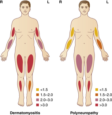
With muscle ultrasound one can also describe the pattern of muscle involvement throughout the body, which may help in the differential diagnosis (Fig. 3.16).44–46 When there is selective involvement of specific muscle groups or regions, muscle ultrasound can identify the diseased muscles and subsequently direct muscle biopsy.47 It is important, however, to avoid biopsy of too severely affected muscles, because pronounced atrophy or fibrosis can lead to sampling errors and difficulties in interpreting the results.45
Interpretation of Muscle Thickness
Muscle atrophy is often found in neuromuscular disorders. However, patients with symptoms such as hypotonia and delay in motor development without a neuromuscular disorder often show muscle atrophy, which is explained by disuse. Exercise and body composition also influence muscle thickness and should be taken into account when interpreting the results. For example, atrophy of the quadriceps muscle in wheelchair-bound patients is not surprising and will therefore not help in determining whether a neuromuscular disorder is present. True hypertrophy can also be found in both healthy subjects (as a training effect) and patients with a neuromuscular disorder, such as myotonia congenita or Brody’s disease. Increased muscle thickness also can be caused by pseudohypertrophy, such as that found in the calves of Duchenne’s muscular dystrophy patients. Muscle thickness will therefore have to be interpreted in combination with the results of quantitative echogenicity measurements. If atrophy is present, an increased muscle echogenicity indicates that the atrophy is probably caused by a neuromuscular disorder, whereas a normal echogenicity is suggestive of disuse atrophy (Table 3.3).
Table 3.3 Interpretation of Muscle Thickness in Correlation with Muscle Echogenicity Findings
| Atrophy | Hypertrophy | |
|---|---|---|
| Normal echogenicity |
Muscle Ultrasound in Clinical Practice: Measurement Protocol
Transducer and System Settings
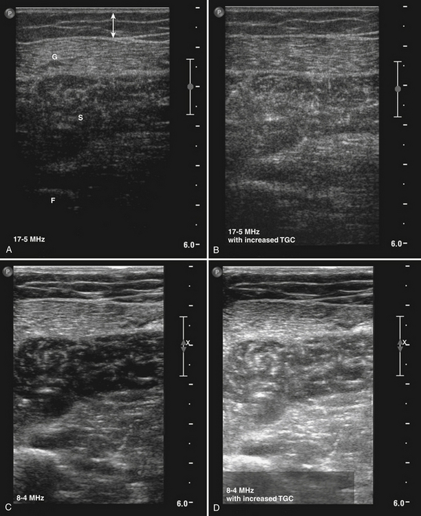
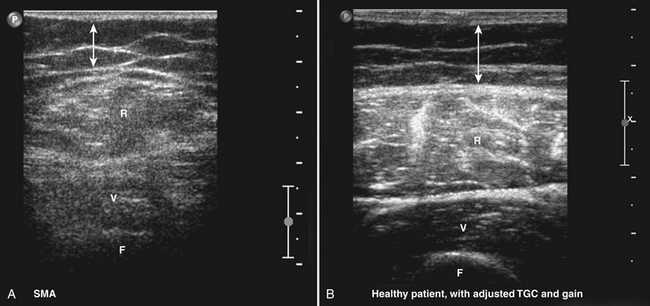
The appropriate transducer to perform muscle ultrasound in children and superficial muscles in adults is a 7.5-MHz probe, and a 5-MHz probe for deeper muscles of adults. A single broadband transducer with a range of at least 12-7 MHz also can be used. It is important to select the optimal settings for the visualization of skeletal muscles. Gain and compression have to be chosen so they will result in a picture in which a normal muscle is relatively black (see Fig. 3.10). This ensures that diseased muscles will appear whiter on the ultrasound screen. Conversely, when the gain is already set too high at the start of the examination, normal muscle tissue will already appear white. If a diseased muscle is then displayed, this muscle will also be white on the screen. Therefore, less contrast between normal and diseased muscle will be available for their discrimination (Fig. 3.17), resulting in a loss of sensitivity and specificity. Focus has to be adjusted to a depth where the muscle of interest is expected. Normally, two or three focal points at 1 to 3 cm deep will be sufficient. It is important to save these settings in a default, often called “preset,” making sure that every measurement will be performed with the same system settings. Such a preset is necessary when one wants to compare measurements between different patients or subjects and makes it possible to familiarize oneself with the normal appearance of muscle and the difference with diseased muscles. If muscle echogenicity is quantified it is mandatory to keep all system settings constant, otherwise the measurements are not comparable. Another adjustment, the so-called time gain compensation, is automatically applied to the ultrasound image by the ultrasound system but can also be further adjusted manually by an operator to obtain the desired image quality on the screen. This adjustment is forbidden when measuring muscle echogenicity quantitatively. When performing quantitative muscle ultrasound measurements one has to be sure that the bars of the time gain compensation are in the same (neutral) position, to be able to compare muscle echo intensities between measurements.
Measurement Errors
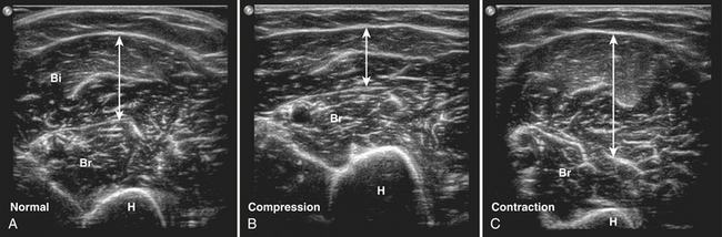
The patient has to be placed in a relaxed position to avoid muscle contraction, because contraction of a muscle results in an increased muscle diameter and a decreased echogenicity (Fig. 3.18).48 To compare muscle thickness or muscle echogenicity between subjects and over time, all measurements have to be performed at the same anatomically defined locations with the subject in a standardized position. For example, bending the knee will cause a change of the direction of the muscle fibers in the quadriceps muscle, resulting in an increased muscle echogenicity compared with measuring echogenicity with a straight leg.1,42
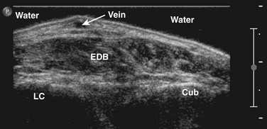
A generous amount of contact gel between the skin and transducer should be used to ensure optimal acoustic coupling and to prevent pressure on the underlying tissues (see Fig. 3.18). Occasionally, a water bath (i.e., immersion of the limb) is necessary when imaging superficial or sharply contoured structures such as muscles of the hand and foot (Fig. 3.19). Especially when measuring in a transverse plane, it is important to place the transducer perpendicular to the underlying muscle tissue, because oblique scanning will not only overestimate muscle thickness but also result in a decrease of muscle echogenicity (see Fig. 3.4).48 Placing the transducer in a way that results in an optimal bone echo and delineation of the surrounding fascia will further standardize the measurement, thereby avoiding differences caused by angulation of the transducer.
All measurement errors and ways to avoid them are summarized in Table 3.4.
Table 3.4 Checklist for Evaluating the Quality of Muscle Ultrasound Measurement
| Measurement error | Check for |
|---|---|
| Incorrect system settings | Check if the correct transducer and preset are selected and if the correct (standard) values for gain, compression, and focal points are visible in the image. |
| Too much pressure exerted | The outline of the skin has to be slightly convex. |
| Not perpendicular to the underlying bone | The bone echo and fascia have to be clearly visible unless a strongly increased echogenicity is present. |
| Air artifacts | The entire image has to be of the same quality without vertical black lines indicating air artifacts. |
| Movement artifacts | The resolution of the image has to be approximately the same in all images. If the muscles have a “fuzzy” appearance, the patient probably was not fully relaxed when the image was captured. Such a measurement should be excluded from further analysis. |
| Incorrect caliper position for measuring muscle thickness | Identify the correct muscle and check for the accurate caliper position. Recalculate if necessary. |
| Incorrect position of region of interest for measuring muscle echogenicity | Identify the correct muscle. The region of interest has to contain almost the entire muscle area but surrounding fascia have to be excluded. |
| Increased attenuation decreasing mean muscle echogenicity | Strong attenuation of the ultrasound beam occurs in severe neuromuscular disorders and can be identified by a very bright superficial part of the muscle that gradually decreases in deeper parts. This feature should be noticed because it will falsely lower the mean echogenicity. |
| Reflective structures superficial or in the muscle | Reflective structures such as calcifications are visible as bright spots with a black line underneath. It will falsely lower the mean echogenicity. |
Quantifying Muscle Ultrasound
Measuring Muscle Thickness
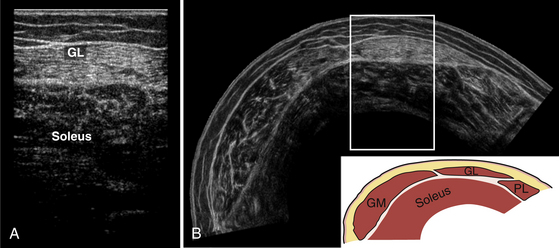
Muscle thickness is usually determined during the measurement, with a caliper function that is generally incorporated in the ultrasound device’s software. In most circumstances, assessment of muscle thickness will be sufficient to determine whether muscle atrophy or hypertrophy is present, but it is also possible to measure muscle cross-sectional area. This type of measurement has become a standard feature in newer ultrasound devices. Measurement of muscle cross-sectional area can have additional value in, for example, the estimation of total muscle mass,17 or to relate the force-generating capacity of muscle to its cross-sectional area.49 The assessment of the cross-sectional area can be done easily in small muscles, when the whole muscle width is visible on the screen. However, larger muscles such as the rectus femoris or biceps brachii muscle often do not fit the size of the transducers (normally 4 to 5 cm wide) and can therefore not be visualized in one image except when they are severely atrophic, or in neonates. Additional image processing such as the panoramic view is then necessary to visualize the entire muscle (Fig. 3.20).50
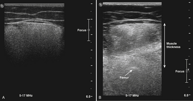
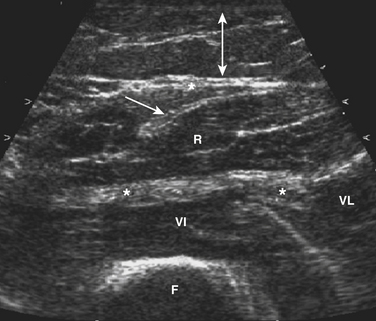
It is advisable to measure muscle thickness from the skin to a highly reflective structure beneath the muscle such as an underlying bone, because other structures such as the surrounding fascia can be difficult to recognize in severe neuromuscular disorders. This might imply that to measure muscle thickness it is necessary to include more than one muscle in the measurement, for example, the rectus femoris and vastus intermedius, when measuring the quadriceps. The underlying bone remains detectable in most circumstances. In some conditions such as severe neuromuscular disorders or obesity, it might be necessary to adjust the system settings only for the purpose of thickness measurement to visualize the bone (for example, by increasing time gain compensation, adjusting the focus, or using a transducer with a lower frequency) (Fig. 3.21).
Measuring Muscle Echogenicity Using Gray Scale Analysis
When quantifying echogenicity it is important to keep all settings that influence the gray value—such as the gain, compression, focus, and time gain compensation—constant throughout the measurements. Slight changes of the probe position already induce some variation in muscle echogenicity. To obtain the most reliable echogenicity it is preferable to make at least three images of each muscle and average the results of all three measurements. This reduces measurement variation. Between each measurement the subject is allowed to move and the transducer has to be repositioned for each new image. The images are then stored for offline calculation of mean muscle echogenicity.
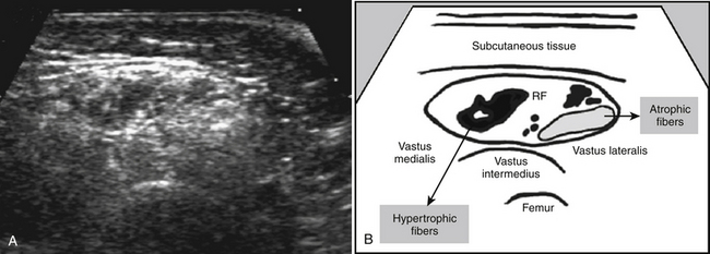
The region of interest preferably consists of a large area within the muscle of interest to avoid sampling errors. In the case of a patchy ultrasound appearance such as spinal muscular atrophy (Fig. 3.22), sampling error can occur when a relatively black part of the muscle is selected. The surrounding fascia should be avoided and not be incorporated in the region of interest because this can falsely elevate muscle echogenicity.
Unfortunately, the muscle echogenicity value is highly dependent on the type of ultrasound device and the system settings used. It is therefore not possible to use normal values established on one device on another device without the help of a correction. Fortunately the mean muscle echogenicity is a solid variable, probably because it is calculated from a rather large area and mainly influenced by the macrotexture of an image that remains approximately the same with different ultrasound devices. This makes it possible to achieve a reliable conversion of normal values after using a conversion equation.51 Such a conversion is made by measuring the same tissue or phantom on the two different ultrasound devices and comparing the results. For converting echogenicity values, one should refrain from additional postprocessing such as compound imaging or other resolution enhancement settings to minimize the difference between ultrasound devices. It is also advisable to perform quality checks of the ultrasound device on occasion to ensure that previously established normal values can still reliably be used.
Visual Assessment of Muscle Ultrasound Images
Muscle ultrasound images can contain additional clues to a specific type of neuromuscular disorder. In Chapters 8 through 10, these features are described for motor neuron disease and specific myopathies. These features cannot be quantified (yet) and can therefore currently only be assessed by visual inspection of the ultrasound images.
For visual assessment, first the distribution of echogenicities within the muscle has to be evaluated: is it homogeneous or inhomogeneous? If inhomogeneous, does the image contain focal areas of increased muscle echogenicity that become especially apparent with angulation of the transducer, pointing to an inflammatory myopathy? Or is it a moth-eaten appearance containing very black areas that can be found in spinal muscular atrophy (see Fig. 3.22)? Table 3.5 summarizes several patterns of echogenicity distribution and the corresponding possible diagnoses.
| Echogenicity Distribution Throughout and Surrounding the Muscle | Possible Diagnosis |
|---|---|
| Homogeneous with attenuation of the ultrasound beam | Muscular dystrophy |
| Focally increased echogenicity especially with angulation of the transducer | Inflammatory myopathies |
| Moth-eaten pattern with severe atrophy | Spinal muscular atrophy |
| Increased echogenicity in an “outside-in fashion,” especially surrounding intramuscular fascia | Bethlem myopathy, Ullrich muscular dystrophy |
| Thickened fascia with unclear demarcation | Fasciitis |
The fascia surrounding the muscle should also be evaluated: is it thin and clearly demarcated (i.e., normal) or thickened with a fuzzy appearance suggestive of a fasciitis (Fig. 3.23)? One should further screen the entire muscle for the presence of subcutaneous and intramuscular calcifications, especially when dermatomyositis is suspected.
Dynamic Muscle Ultrasound
Unlike other imaging techniques such as MRI and computed tomography (CT), ultrasound is the only technique that routinely results in more than static pictures. Its unique property to display real-time pictures increases its diagnostic capabilities. When the repetition frequency of the pictures on the display screen is higher than 15 frames per second it appears as real-time to our visual system. Modern ultrasound machines have this capability—and physiologic and pathologic muscle movements can be detected.13,14,52,53 Early studies have mainly focused on the detection of fasciculations by ultrasound, showing even higher sensitivities than needle EMG or clinical investigation.52–55 Developments in ultrasound techniques, with improved spatial resolution and the frame rate, have made it possible to detect smaller movements such as fibrillations,56–57 which was previously considered to be impossible.53 Many different abnormal movements due to disorders of the peripheral nervous system can be detected with muscle ultrasound (Table 3.6). However, up until now most have not systematically been studied; therefore, only fasciculations and fibrillations are discussed in detail in this chapter.
Table 3.6 Pathologic Findings and Pitfalls in Dynamic Muscle Ultrasound
| Movement | Ultrasound Appearance |
|---|---|
| PATHOLOGIC MUSCLE MOVEMENT | |
| Fasciculation | Short jerky movement in focal areas of the muscle. Often not confined to one area. The overall shape of the muscles can be slightly disturbed, depending on the amount and location of the fasciculations (see Video 3.2) |
| Myokymia | Short jerky movements confined to one area of the muscle |
| Fibrillations | Small, irregularly oscillating movements within the muscle while the overall shape of the muscle remains undisturbed (see Video 3.5) |
| Contraction pseudotremor | Small- to medium-sized rhythmic oscillating movements that can resemble fibrillations or fasciculations but disappear on relaxation of the muscle (see Video 3.4) |
| PITFALLS | |
| Arterial pulsation | Rhythmic contraction confined to one area (see Video 3.3). Application of Doppler imaging reveals blood flow. |
| Voluntary muscle contraction | Movement comprising the entire muscle with altering of the overall shape (see Video 3.1). |
| Movement of transducer | Displacement of muscle tissue and surrounding tissue in equal amounts. |
Contraction of the Entire Muscle
A normal voluntary contraction can easily be evoked and studied. It should be realized that during a normal contraction the firing of motor units is such that shortening of the muscle appears as a smooth movement. Individual motor units cannot be visualized at current ultrasound resolution. During contraction, the muscle shape changes, resulting in an increased cross-sectional area with decreased echogenicity. Smoother voluntary contractions can easily be differentiated from pathologic spontaneous muscle movements, such as fasciculations, that result in jerky, short, and local movements. Video 3.1 shows an example of a normal contracting biceps brachii muscle. During contraction of this muscle, the fascia dividing the medial, and lateral head of the biceps becomes visible.
Different involuntary movements such as tremor, cramp, myoclonus, and chorea can be visualized using ultrasound.53 Tremors are repetitive, rhythmic, involuntary muscle contractions, often leading to oscillating movements of parts of the body. Tremor is associated with many neurologic disorders and can be the only clinical sign (as in essential tremor), or be part of a neurologic syndrome (e.g., Parkinson’s disease). Furthermore, tremor can also occur in healthy people as an exaggerated physiologic tremor. On muscle ultrasound, tremor is recognized as rhythmic contractions of the entire muscle. The observed movements on ultrasound may change according to the anatomic position of the extremity or depend on the posture of the patient. It has been shown that dynamic muscle ultrasound can be used to estimate the tremor frequency.58
When studying patients with cramp, chorea, or myoclonus, the muscle contracting can be identified and visualized, but because the ultrasound appearance is essentially the same for all contractions, differentiation from voluntary contractions based on dynamic muscle ultrasound alone is not possible.53
Fasciculations
Fasciculations are random, spontaneous contractions of the muscle fibers of a single motor unit. They are caused by a variety of reasons,59 with affection of a part of the lower motor neuron as the common characteristic. Diseases in which fasciculations can be seen include motor neuron disease, various neuropathies, myelopathy, and toxic syndromes. Their occurrence and distribution can be important diagnostic clues, especially in amyotrophic lateral sclerosis.60 Superficial fasciculations can be seen through the skin as a contraction of a small part of the muscle. If they are generated in deeper parts of the muscle, fasciculations can only be detected by EMG or muscle ultrasound.
Fasciculations can also occur as a benign phenomenon found in many healthy people, mainly in the calf and intrinsic foot muscles.52,54,61,62 The prevalence of fasciculations increases with age and strenuous physical exercise. They usually do not occur in muscles above the knee.63
On ultrasound, fasciculations appear as spontaneous–focal jerky movements that occur irregularly and randomly in different parts of the muscle (see Video 3.2). They are easily recognized, especially when screening in a transverse plane, as a focal muscle thickening in both the horizontal and vertical directions. In a longitudinal plane only a vertical thickening can be seen, which makes it slightly more difficult to identify fasciculations in longitudinal scans.
Several studies have investigated the sensitivity in detection of fasciculations by ultrasound.52,55,62 The area of muscle that is examined during needle EMG is very small compared with the area that can be visualized using ultrasound.55 With ultrasound the entire transverse plane of a muscle can usually be screened for fasciculations simultaneously. This is the main reason that the sensitivity for detecting fasciculations using ultrasound is higher than needle EMG or visual inspection of the skin.52–5564 Moreover, fasciculations can still be recognized during voluntary muscle contraction, something that is not possible with EMG because of the summation of electrical potentials recorded by the needle electrode.55 The specificity of ultrasound equals that of visual inspection (86%).52 Recognition is relatively easy with an interobserver agreement of 0.84 to 0.85, which is comparable with the recognition of fasciculations by EMG.52,62
To detect any fasciculations present, ultrasound screening has to be performed for a sufficient period of time. In one study, 77% of the observed fasciculations occurred with a frequency of more than one per 2 seconds.52 This frequency was not related to the muscle studied. It can be calculated that screening a single muscle for 8 seconds yields a sensitivity of 95% to detect any fasciculations.52 Most authors, however, recommend a screening duration of 10 seconds.
Offline analysis of the ultrasound video allows for measurements of the cross-sectional area of a fasciculation and its temporal profile.55 The cross-sectional area of a single fasciculation was shown to be different for smaller and larger muscles, with mean areas of 5.5 ± 3.3 mm2 in the first dorsal interosseous and 58 ± 18 mm2 in the gastrocnemius muscle. In patients with electromyographic evidence of reinnervation, particularly in post-polio patients, the area can be up to 109 mm2.55 The duration of a single fasciculation is 500 ± 110 ms, including a contractile phase, a plateau phase, and a relaxation phase.55
Several pitfalls have to be taken into account when screening for fasciculations. Shivering and voluntary contractions may be mistaken for fasciculations, but in contrast to fasciculations involve the entire cross-sectional area of the muscle. However, in the case of several small muscles within a muscle group, such as the forearm flexors, the differentiation between short voluntary contractions and fasciculations can be difficult. A careful observation of the patient and reevaluation of the muscle when fully relaxed will usually solve this problem. Arterial pulsations are visible as small movements within muscle that can be easily differentiated from fasciculations, because they are rhythmic and unifocal (see Video 3.3). When in doubt, color Doppler imaging will easily tell them apart. Another pitfall can occur in patients with chronic denervation and collateral reinnervation of muscle fibers, leading to very large motor units. In these patients, slight voluntary contraction leading to activation of only one or two large motor units may resemble fasciculations clinically as well as on ultrasound. This clinical phenomenon is often referred to as contraction pseudotremor or contraction fasciculations. Prolonged contraction in these cases can also appear as fibrillations (see next section; also see Video 3.4). The main differentiation between fasciculations and contraction pseudotremor can be made on the response to contraction and relaxation: fasciculations do not disappear on relaxation, whereas contraction pseudotremor does. Additionally, contraction pseudotremor causes intramuscular movements that remain in the same place, whereas fasciculations appear randomly throughout the muscle. If questions remain, surface or needle EMG may be informative.
Fibrillations
Fibrillations are spontaneous depolarizations of the membrane of individual muscle fibers that result in contraction of an individual fiber. They result from the fiber’s loss of contact with its innervating axon.65 For this reason fibrillations are an important sign of axonal loss in peripheral nerve disorders, but they can also occur in myopathies when muscle fibers are split or inflammation is present that separates part of the fiber from the endplate zone. Because fibrillations are invisible from the outside, they can only be detected by needle EMG and appear as spontaneous single-action potentials. New developments in ultrasound techniques, resulting in better resolution and higher frame rates, have made it possible to visualize fibrillations.56,57 Although single muscle fibers are too small to visualize individually with the current maximal ultrasound resolution, fibrillating muscle fibers cause enough displacement of their surrounding tissue to be detectable. Fibrillations appear on the ultrasound video as small, irregularly oscillating movements of muscle tissue in all directions, while the overall shape of the muscle is preserved (see Video 3.5). One study indicated that the sensitivity of ultrasound for detecting fibrillations depends on the amount of fibrillations present and, critically, on limb temperature.57 Ultrasound was found incapable of detecting fibrillations when EMG recorded less than 5 fibrillation potentials per second, and the visualization of movements decreased steeply below 30° C. However, EMG, which is the gold standard for fibrillation detection, can also miss focal areas with fibrillations within muscle because of sampling error, and here ultrasound has the advantage of visualizing larger areas of the muscle to help avoid this problem.
The detection of fibrillations is susceptible to several pitfalls. Artifacts caused by external movements or ultrasound noise caused by scattering on bone can be mistaken for fibrillations. Table 3.7 summarizes the main pitfalls in the detection of fibrillations and the methods used to avoid them.
Table 3.7 Pitfalls in the Detection of Fibrillations and the Methods used to Avoid Them
| Pitfall | Method for Improvement |
|---|---|
| PITFALLS RESEMBLING FIBRILLATIONS | |
| External movement artifacts | |
Dynamic Ultrasound in Clinical Practice
To ensure optimal measurement, care has to be taken to instruct the patient to fully relax his or her muscles. The position of the patient should also be taken into account because some positions cause unintentional muscle contractions, for example, supination of the forearm is involuntarily accompanied by contraction of the supinator muscle. During the ultrasound measurement special attention has to be given to pathologic muscle movements that could signify a specific neuromuscular disorder. At rest, the presence of pathologic spontaneous muscle activity such as fasciculations and fibrillations should be evaluated. Patients can be asked to contract a specific muscle to judge whether a normal contraction pattern is present. If possible one should compare this with the contralateral side.
The examiner needs to gain experience in the different muscle ultrasound appearances of both normal and pathologic movements. During this learning phase it is advisable to verify the ultrasound findings by needle EMG investigation to check if the correct interpretation has been made. Table 3.6 summarizes the main pitfalls that can be encountered in dynamic muscle ultrasound.
1. Heckmatt J.Z., Dubowitz V., Leeman S. Detection of pathological change in dystrophic muscle with B-scan ultrasound imaging. Lancet. 1980;1:1389-1390.
2. Campbell S.E., Adler R., Sofka C.M. Ultrasound of muscle abnormalities. Ultrasound Q. 2005;21:87-94.
3. Fornage B.D. The case for ultrasound of muscles and tendons. Semin Musculoskelet Radiol. 2000;4:375-391.
4. Hashimoto B.E., Kramer D.J., Wiitala L. Application of musculoskeletal sonography. J Clin Ultrasound. 1999;27:293-299.
5. Peetrons P. Ultrasound of muscles. Eur Radiol. 2002;12:35-43.
6. Cosgrove D. Ultrasound: general principles. In: Grainger R.G., Allison D.J., editors. Diagnostic radiology. Edinburgh, UK: Churchill Livingstone; 1992:65-77.
7. Saupe N., Prüssmann K.P., Luechinger R., et al. MR imaging of the wrist: comparison between 1.5- and 3-T MR imaging: preliminary experience. Radiology. 2005;234:256-264.
8. Fish P. Diagnostic medical ultrasound. Chichester: John Wiley & Sons Ltd; 1990.
9. Shirley I.M., Blackwell R.J., Cusick G., et al. A user’s guide to diagnostic ultrasound. Tunbridge Wells: Pitman Medical Publishing Co Ltd; 1978.
10. Engel A.G., Banker B.Q. Myology. New York: McGraw-Hill; 1986.
11. Junqueira L.C., Carneiro J., Kelley R.O.. Basic histology, East Norwalk, Conn, ed 8, 1995, Appleton & Lange.
12. Moore K.L. Clinical oriented anatomy, ed 3. Baltimore: Williams & Wilkins; 1992.
13. Pillen S., Arts I.M.P., Zwarts M.J. Muscle ultrasound in neuromuscular disorders. Muscle Nerve. 2008;37:679-693.
14. Walker F.O., Cartwright M.S., Wiesler E.R., Caress J. Ultrasound of nerve and muscle. Clin Neurophysiol. 2004;115:495-507.
15. Reeves N.D., Maganaris C.N., Narici M.V. Ultrasonographic assessment of human skeletal muscle size. Eur J Appl Physiol. 2004;91:116-118.
16. Reimers C.D., Harder T., Saxe H. Age-related muscle atrophy does not affect all muscles and can partly be compensated by physical activity: an ultrasound study. J Neurol Sci. 1998;159:60-66.
17. Sanada K., Kearns C.F., Midorikawa T., Abe T. Prediction and validation of total and regional skeletal muscle mass by ultrasound in Japanese adults. Eur J Appl Physiol. 2006;96:24-31.
18. Reimers C.D., Schlotter B., Eicke B.M., Witt T.N. Calf enlargement in neuromuscular diseases: a quantitative ultrasound study in 350 patients and review of the literature. J Neurol Sci. 1996;143:46-56.
19. Scholten R.R., Pillen S., Verrips A., Zwarts M.J. Quantitative ultrasonography of skeletal muscles in children: normal values. Muscle Nerve. 2003;27:693-698.
20. Arts I.M., Pillen S., Overeem S., et al. Rise and fall of skeletal muscle size over the entire life span. J Am Geriatr Soc. 2007;55:1150-1152.
21. Kanehisa H., Ikegawa S., Tsunoda N., Fukunaga T. Cross-sectional areas of fat and muscle in limbs during growth and middle age. Int J Sports Med. 1994;15:420-425.
22. Kanehisa H., Yata H., Ikegawa S., Fukunaga T. A cross-sectional study of the size and strength of the lower leg muscles during growth. Eur J Appl Physiol Occup Physiol. 1995;72:150-156.
23. Arts I.M., Pillen S., Schelhaas H.J., et al. Normal values for quantitative muscle ultrasonography in adults. Muscle Nerve. 2010;41:32-41.
24. Doherty T.J. Invited review: aging and sarcopenia. J Appl Physiol. 2003;95:1717-1727.
25. Maurits N.M., Bollen A.E., Windhausen A., et al. Muscle ultrasound analysis: normal values and differentiation between myopathies and neuropathies. Ultrasound Med Biol. 2003;29:215-225.
26. Reimers C.D., Fleckenstein J.L., Witt T.N., et al. Muscular ultrasound in idiopathic inflammatory myopathies of adults. J Neurol Sci. 1993;116:82-92.
27. Pillen S., Scholten R.R., Zwarts M.J., Verrips A. Quantitative skeletal muscle ultrasonography in children with suspected neuromuscular disease. Muscle Nerve. 2003;27:699-705.
28. Aydinli N., Baslo B., Caliskan M., et al. Muscle ultrasonography and electromyography correlation for evaluation of floppy infants. Brain Dev. 2003;25:22-24.
29. Fischer A.Q., Carpenter D.W., Hartlage P.L., et al. Muscle imaging in neuromuscular disease using computerized real-time sonography. Muscle Nerve. 1988;11:270-275.
30. Pillen S., Keimpema M., Nievelstein R.A.J., et al. Skeletal muscle ultrasonography: visual versus quantitative evaluation. Ultrasound Med Biol. 2006;32:1315-1321.
31. Bargfrede M., Schwennicke A., Tumani H., Reimers C.D. Quantitative ultrasonography in focal neuropathies as compared to clinical and EMG findings. Eur J Ultrasound. 1999;10:21-29.
32. Heckmatt J., Rodillo E., Doherty M., et al. Quantitative sonography of muscle, J Child Neurol, Suppl 4, 1989, S101-S106.
33. Zaidman C.M., Holland M.R., Anderson C.C., Pestronk A. Calibrated quantitative ultrasound imaging of skeletal muscle using backscatter analysis. Muscle Nerve. 2008;38:893-898.
34. Pohle R., Fischer D., von Rohden L. Computer-supported tissue characterization in musculoskeletal ultrasonography. Ultraschall Med. 2000;21:245-252.
35. Chen C.M., Chou Y.H., Han K.C., et al. Breast lesions on sonograms: computer-aided diagnosis with nearly setting-independent features and artificial neural networks. Radiology. 2003;226:504-514.
36. Loch T., Leuschner I., Genberg C., et al. Artificial neural network analysis (ANNA) of prostatic transrectal ultrasound. Prostate. 1999;39:198-204.
37. Pillen S., Verrips A., van Alfen N., et al. Quantitative skeletal muscle ultrasound: diagnostic value in childhood neuromuscular disease. Neuromuscul Disord. 2007;17:509-516.
38. Reimers K., Reimers C.D., Wagner S., et al. Skeletal muscle sonography: a correlative study of echogenicity and morphology. J Ultrasound Med. 1993;12:73-77.
39. Pillen S., Tak R., Lammens M., et al. Skeletal muscle ultrasound: correlation between fibrous tissue and echogenicity. Ultrasound Med Biol. 2009;35:443-446.
40. Brockmann K., Becker P., Schreiber G., et al. Sensitivity and specificity of qualitative muscle ultrasound in assessment of suspected neuromuscular disease in childhood. Neuromuscul Disord. 2007;17:517-523.
41. Heckmatt J.Z., Pier N., Dubowitz V. Real-time ultrasound imaging of muscles. Muscle Nerve. 1988;11:56-65.
42. Zuberi S.M., Matta N., Nawaz S., et al. Muscle ultrasound in the assessment of suspected neuromuscular disease in childhood. Neuromuscul Disord. 1999;9:203-207.
43. Pillen S., Morava E., Van Keimpema M., et al. Skeletal muscle ultrasonography in children with a dysfunction in the oxidative phosphorylation system. Neuropediatrics. 2006;37:142-147.
44. Heckmatt J.Z., Dubowitz V. Ultrasound imaging and directed needle biopsy in the diagnosis of selective involvement in muscle disease. J Child Neurol. 1987;2:205-213.
45. Lindequist S., Larsen C., Daa S.H. Ultrasound guided needle biopsy of skeletal muscle in neuromuscular disease. Acta Radiol. 1990;31:411-413.
46. O’Sullivan P.J., Gorman G.M., Hardiman O.M., et al. Sonographically guided percutaneous muscle biopsy in diagnosis of neuromuscular disease: a useful alternative to open surgical biopsy. J Ultrasound Med. 2006;25:1-6.
47. Heckmatt J.Z., Dubowitz V. Diagnostic advantage of needle muscle biopsy and ultrasound imaging in the detection of focal pathology in a girl with limb girdle dystrophy. Muscle Nerve. 1985;8:705-709.
48. Heckmatt J.Z., Pier N., Dubowitz V. Measurement of quadriceps muscle thickness and subcutaneous tissue thickness in normal children by real-time ultrasound imaging. J Clin Ultrasound. 1988;16:171-176.
49. Clague J.E., Roberts N., Gibson H., Edwards R.H. Muscle imaging in health and disease. Neuromuscul Disord. 1995;5:171-178.
50. Chi-Fishman G., Hicks J.E., Cintas H.M., et al. Ultrasound imaging distinguishes between normal and weak muscle. Arch Phys Med Rehabil. 2004;85:980-986.
51. Pillen S., Van Dijk J.P., Weijers G., et al. Quantitative grey scale analysis in skeletal muscle ultrasound: a comparison study of two ultrasound devices. Muscle Nerve. 2009;39:781-786.
52. Reimers C.D., Ziemann U., Scheel A., et al. Fasciculations: clinical, electromyographic, and ultrasonographic assessment. J Neurol. 1996;243:579-584.
53. Scheel A.K., Reimers C.D. Detection of fasciculations and other types of muscular hyperkinesias with ultrasound. Ultraschall Med. 2004;25:337-341.
54. Scheel A.K., Toepfer M., Kunkel M., et al. Ultrasonographic assessment of the prevalence of fasciculations in lesions of the peripheral nervous system. J Neuroimaging. 1997;7:23-27.
55. Walker F.O., Donofrio P.D., Harpold G.J., Ferrell W.G. Sonographic imaging of muscle contraction and fasciculations: a correlation with electromyography. Muscle Nerve. 1990;13:33-39.
56. van Baalen A., Stephani U. Fibration, fibrillation, and fasciculation: say what you see. Clin Neurophysiol. 2007;118:1418-1420.
57. Pillen S., Nienhuis M., van Dijk J.P., et al. Muscles alive: ultrasound detects fibrillations. Clin Neurophysiol. 2009;120:932-936.
58. Walker F.O. Muscle ultrasound: an AAEM workshop. Rochester, Minn: American Association of Electrodiagnostic Medicine; 1998.
59. Desai J., Swash M. Fasciculations: what do we know of their significance? J Neurol Sci. 1997;152(Suppl 1):S43-S48.
60. Arts I.M., van Rooij F.G., Overeem S., et al. Quantitative muscle ultrasonography in amyotrophic lateral sclerosis. Ultrasound Med Biol. 2008;34:354-361.
61. Reed D.M., Kurland L.T. Muscle fasciculation in a healthy population. Arch Neurol. 1963;9:363-367.
62. Wenzel S., Herrendorf G., Scheel A., et al. Surface EMG and myosonography in the detection of fasciculations: a comparative study. J Neuroimaging. 1998;8(3):148-154.
63. Fermont J., Arts I.M., Overeem S., et al. Prevalence and distribution of fasciculations in healthy adults: effect of age, caffeine consumption and exercise. Amyotroph Lateral Scler. 2009;15:1-6.
64. Howard R.S., Murray N.M. Surface EMG in the recording of fasciculations. Muscle Nerve. 1992;15:1240-1245.
65. Buchthal F., Rosenfalck P. Spontaneous electrical activity of human muscle. Electroencephalogr Clin Neurophysiol. 1966;20:321-336.