Chapter 12
Teaching Visual: How to Interpret an Electrocardiogram
Jessica L. Israel MD
Objectives
 Develop a systematic approach to ECG interpretation.
 Create a narrative description of ECG findings.
 Apply this systematic approach and narrative description techniques to the interpretation of three commonly encountered ECGs and two rhythm strips.
INTRODUCTION: WHO SHOULD HAVE AN ECG?
The ECG is one of the hallmarks of cardiac diagnostic testing. Interestingly, many hospitalized patients will have ECGs recorded upon admission, and many will have “baseline” ECGs filed in their outpatient charts. However, the US Preventive Services Task Force recommends against screening for coronary heart disease in low-risk adults. There is also no clear evidence that screening helps predict the progression of disease in high-risk adults (http://www.uspreventiveservicestaskforce.org/).
In general, ECGs should be done for patients with cardiac complaints or in those who present with related complaints secondary to other cardiovascular or pulmonary disease. Outpatient ECGs are helpful to document a known ECG abnormality, which may serve as a useful comparison in the future, and for preoperative screening in the appropriate patient.
DEVELOPING A SYSTEMATIC APPROACH
For most internists, ECG interpretation is a common task in patient care. However, even the most experienced internists may need consultation with a colleague to analyze a complicated tracing. Developing a systematic approach to ECG interpretation helps to ensure that you look at all of the aspects of the tracing (not just the obvious ones); even if you are unsure what the underlying problem may be, you will still be able to systematically describe your findings to a colleague in consultation. This overview is a guide to reading ECGs and is by no means exhaustive. However, you can learn by simply applying this rubric over and over again. In moments that are not so busy during your medicine rotation, one useful exercise is to pull multiple ECG tracings from the charts of patients and review them, perhaps even with the help of a resident. The more ECGs you read, the more comfortable you will be interpreting them.
P waves, T waves, and QRS complexes appear differently in each of the 12 standard ECG leads. The P waves, T waves, and QRS complexes have been labeled in lead II in Figure 12-1. Label them for leads aVR and V6.
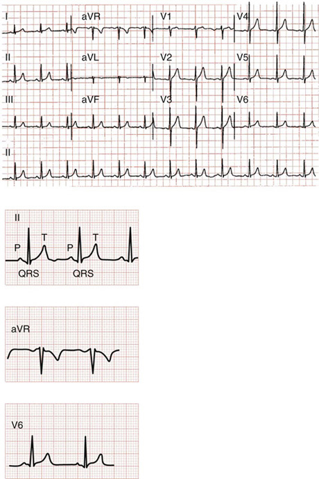
Figure 12-1 (From Goldberger AL. Clinical electrocardiography: a simplified approach. 7th ed. Philadelphia: Mosby; 2006, p. 44, question 1.)
Step 4: Hypertrophy/chamber size
Step 5: Ischemic changes/infarction
Step 1: Determining the Rate
To calculate the rate, find an R wave that is lined up with a heavy border of a background grid box. After this, you simply count down until your next R wave appears. The counting is specific: the distance to the next grid line is 300 bpm, to the second grid line is 150 bpm, the third is 100 bpm, the fourth is 75 bpm, the fifth is 60 bpm, and the sixth is 50 bpm. Often the next R wave will appear between two major grid lines, and in these cases you simply estimate the rate. For example, if your rate determination falls exactly between the 75 and the 60 line, you can perhaps estimate the heart rate at 68 bpm. Note: to be precise the distance between two heavy grid lines is 1/300 of a minute. Therefore, the distance between two heavy grid lines is 2/300, and three grid lines is 3/300, which can be simplified to 1/150 and 1/100, respectively. That’s where these numbers come from, so committing them to memory can be helpful.
If the heart rate is normal at rest, it should fall somewhere between 60 and 100 bpm. If the heart rate is generated from the sinus node, then a slow (or bradycardic) rate is less than 60 bpm. A fast (or tachycardic) rate is greater than 100 bpm. If the sinus node (or another atrial focus) fails to set pace, a junctional automaticity focus would assume the pace; if this focus fails, a ventricular automaticity focus would pace the heart. A junctionally generated rhythm is usually between 40 and 60 bpm. A ventricular focus would generate a rate of 20 to 40 bpm. Rates slower than 50 bpm require counting how many beats occur in a 6-second time period and then multiplying that number by 10.
The rate you determine will become the first part of your systematic description; for example, “The rate is about 75 beats per minute.” Take a moment now to determine the rate in the ECG in Figure 12-1.
Step 2: Determining the Rhythm
After finding the rate, determining the rhythm (i.e., from where the heart rate is being generated) is the next step. Some common rhythms are:
 Sinus rhythm: This rhythm is described as “regular,” meaning the pattern is constant and does not vary. All of the cycles are of equal length. You can tell the rhythm is sinus because every QRS complex is preceded by a P wave, and the P wave and PR interval appear uniform and the same throughout the tracing. Looking at Figure 12-1, locate the P waves before every QRS complex. Then, as you continue your description of the tracing you would add, “The rate is 75 bpm and the rhythm is a normal sinus rhythm.”
 Atrial fibrillation: This rhythm is described as “irregularly irregular,” meaning that there are no predictable recurring features. In atrial fibrillation there are no true P waves at all. There are multiple areas of the atrium that are irritable and setting a pace all at once. Write a description of the rate and rhythm of the ECG rhythm strip in Figure 12-2.
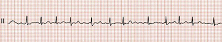
Figure 12-2 (From Goldberger AL. Clinical electrocardiography: a simplified approach. 7th ed. Philadelphia: Mosby; 2006. Figure 15-4.)
Write a description of the rate and rhythm of the ECG rhythm strip in Figure 12-3. This one is atrial fibrillation with a rapid ventricular response.
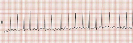
Figure 12-3 (From Goldberger AL. Clinical electrocardiography: a simplified approach. 7th ed. Philadelphia: Mosby; 2006, Figure 15-5.)
 Ventricular tachycardia: Ventricular tachycardias are produced by very irritable foci in the ventricle that produce rapid ventricular rates, usually from 150 to 250 bpm. This rhythm is usually produced by compromised coronary blood flow. There will be no P waves, and the QRS complex will appear wide.
 Ventricular flutter: Here the rate is between 250 and 350 bpm. It looks like a rapid series of sine waves.
 Ventricular fibrillation: This rhythm is totally erratic, with no pattern or consistency. The rate is usually between 350 and 450 bpm.
There are tracings of all three of the ventricular arrhythmias in Figures 12-4 and 12-5. Study the differences in terms of rate.
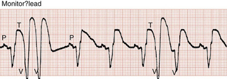
Figure 12-4 (From Goldberger AL. Clinical electrocardiography: a simplified approach. 7th ed. Philadelphia: Mosby; 2006, Figure 16-4.)
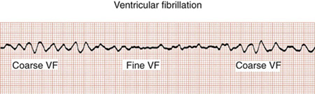
Figure 12-5 (From Goldberger AL. Clinical electrocardiography: a simplified approach. 7th ed. Philadelphia: Mosby; 2006, Figure 16-13.)
Obviously, there are multiple cardiac arrhythmias not demonstrated here. The key to recognizing them is in your description: what the rate is, what waveforms are present, and what those forms look like. For example, looking at the length of the PR interval and the length of the QRS complex can tell you where the focus of the rhythm is originating.
Step 3: Determine the Axis
The axis refers to the direction of depolarization of the heart. One very quick way to determine the axis is to look at two leads: leads I and aVF. In general, if the QRS complex is upward-pointing (or positive) in both of these leads, then the axis is normal. If the QRS is positive in lead I and downward-pointing (or negative) in lead aVF, then there is left-axis deviation. If the axis in lead I is negative but aVF is positive, there is right-axis deviation. If leads I and aVF are both downward-pointing, there is extreme right- or extreme left-axis deviation.
If we now refer to the first ECG tracing in this chapter (see Fig. 12-1), you can continue your description: “The rate is approximately 75 beats per minute, the rhythm is sinus, and the axis is normal.”
Step 4: Look for Hypertrophy and Chamber Size
Corresponding waveforms can provide information about chamber size.
 Atrial enlargement: Leads II and V
 Ventricular hypertrophy: Here we will look at the QRS complex. Look for right ventricular hypertrophy in lead V1: if the S wave is smaller than the R wave, then the right ventricle is hypertrophied; the R waves in leads V2 through V4 will also become progressively smaller. In left ventricular hypertrophy, there will be a deep S wave in V1 and left-axis deviation. There will also be a very tall R wave in V5. If you add the number of smaller grid boxes from the size of the S wave in lead V1 and the size of the R wave in V5 and you find more than 35 boxes, there is left ventricular hypertrophy. You can also look at lead aVL; if the height of the R wave is greater than 11 small grid boxes, there is left ventricular hypertrophy. Examining these features in our original ECG (see Fig. 12-1), the description now reads: “Rate of 75 bpm, sinus rhythm, normal axis with no hypertrophy.”
Step 5: Look for Evidence of Ischemia, Injury, or Infarction
 Ischemia: This means the blood supply to a section of heart is compromised and insufficient. The classic sign of ischemia on an ECG is inverted T waves. Look for this finding in every ECG you read.
 Infarction: Here you will need to examine the ST segments. In a normal ECG (such as in Fig. 12-1), this segment is flat, without a wave to it. When the ST segment is elevated, there is acute injury to the underlying myocardium. It is the earliest sign of a myocardial infarction on the ECG. If the ST segment is elevated without a Q wave, this may be a non–Q-wave infarction. ST segments can also be depressed. This usually happens in patients with subendocardial infarctions that do not extend through the full thickness of the heart wall and is another type of non–Q-wave infarction. Q waves form when an area of the heart becomes necrotic. A significant Q wave is at least one small grid box wide.
 The location of the above findings in particular leads helps to discern the area of the heart that is affected and even the vessel most likely involved.
 Any patient with these findings needs immediate attention in the ER setting.
Create a narrative description for an ECG described as follows: “The rate is approximately 90 bpm, the rhythm is sinus, the axis is normal, there is no hypertrophy, there are ST segment depressions in leads I, II, III, aVL, aVF, and V2 through V6. There are no Q waves.” This is severe subendocardial ischemia (Fig. 12-6).
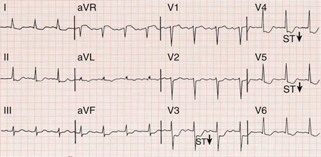
Figure 12-6 (From Goldberger AL. Clinical electrocardiography: a simplified approach. 7th ed. Philadelphia: Mosby; 2006, Figure 9-6.)
