Statistics for the Clinical Scientist

Published on 10/04/2015 by admin

Filed under Surgery

Last modified 22/04/2025

Print this page

This article have been viewed 1885 times

Chapter 9 Statistics for the Clinical Scientist

Harry J. Khamis

INTRODUCTION

Statistics is the science of (1) designing experiments or studies; (2) collecting, organizing, and summarizing data; (3) analyzing data; and (4) interpreting and communicating the results of the analyses. For medical research studies, the data often consist of measurements taken from human subjects (clinical studies) or from animals.

The essential goal of statistics is to make conclusions (or inferences) about a parameter, such as a mean, proportion, regression coefficient, or correlation. The true value of the parameter can be determined by obtaining the measurements of the entire population to which inferences are to be made. However, this is most often impractical or impossible to do. So, instead we take a subset of the population, called a sample. Then we analyze the sample to estimate or test the parameter value. As an example, suppose we would like to know the mean fetal humeral soft tissue thickness (HSTT) of singleton gestations for women at 20 weeks’ gestation. It would be impractical to (sonographically) measure the fetal HSTT for all such women, so we randomly sample, say, 50 such women. We then estimate the mean fetal HSTT from these 50 women. The mean fetal HSTT from these 50 women (called the sample mean) will undoubtedly not be the same as the (theoretical) mean that we would have obtained had we measured all such women (called the population mean), but it should be “close.” How close is it? Would it be closer if we had randomly sampled 100 women? 500 women? These are the questions that the science of statistics is designed to answer.

The next section outlines two essential characteristics of variables. The remaining sections of this chapter present the basic statistical methods used to accomplish the four goals of statistics defined above.

LEVEL OF MEASUREMENT AND VARIABLE STRUCTURE

Any medical research study consists of a set of variables, such as gestational age, birth weight, body mass index (BMI), gender, Bishop score, blood pressure (BP), cholesterol level, severity of disease, dosage level, type of treatment, or type of operation. For statistical purposes, it is important to characterize each variable in two ways: (1) level of measurement and (2) variable structure.

Level of Measurement

The level of measurement (or measurement scale) of a variable is its designation as continuous or discrete. A continuous variable has values taken, at least theoretically, from a continuum of the real number line. Examples are gestational age, BP, and BMI. A discrete variable has discrete values (i.e., values not coming from a continuum of the real number line). Examples are gender (male, female), severity of disease (low, medium, high), and type of operation (standard, modified, laparoscopic). The “severity of disease” variable is called an ordinal discrete variable because there is an order associated with its levels; the “type of operation” variable is called a nominal discrete variable because there is no order associated with its levels.

Variable Structure

A dependent variable (also called outcome, endpoint, or response variable) is the primary variable of a research study. It is the behavior of such a variable that is of primary concern, including the effects (or influence) of other variables on it. An independent variable (also called explanatory, regressor, or predictor variable) is the variable whose effect on the dependent variable is being studied. Designation of which variables are dependent and which are independent in a research study establishes the variable structure. How a variable is handled statistically depends in large part on its level of measurement and its variable structure.¹

EXPERIMENTAL/RESEARCH DESIGN

The three core principles of experimental design are (1) randomization, (2) replication, and (3) control or blocking. Random selection of subjects from the study population or random assignment of subjects to treatment groups is necessary to avoid bias in the results. A random sample of size n from a population is a sample whose likelihood of having been selected is the same as any other sample of size n. Such a sample is said to be representative of the population. See any standard statistics text for a discussion of how to randomize.^2,³

Replication refers to the measurement of subjects under the same condition. This is necessary to determine how the measurements vary for that condition. So, the measurements of several subjects receiving the same treatment would be considered replications.

Control, or blocking, is a technique to adjust an analysis for another variable (sometimes called a confounding variable or covariate). The variability associated with such a variable is accounted for in the analysis in a way that increases the precision of the comparisons of interest. See the discussion of the randomized complete block design for an example.

Completely Randomized Design (CRD)

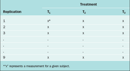
In the CRD, subjects are randomly assigned to experimental groups. As an example, suppose that the thickness of the endometrium is observed via ultrasound for women randomly assigned to three different fertility treatments (treatments T₁, T₂, and T₃). Twenty-seven subjects are available for study, so 9 subjects are randomly selected to receive treatment T₁, 9 are randomly selected from the remaining 18 to receive treatment T₂, and the remaining 9 receive treatment T₃. The data layout appears in Table 9-1.

Table 9-1 Data Layout For a Completely Randomized Design

In addition to randomness, an important assumption of the CRD is that the samples are independent (i.e., the outcome measurement—in this case, endometrial thickness—for one subject is not related to that of any other subject). For instance, two related subjects (e.g., sisters) should not both be included in the data set because they are genetically related and hence their endometrial thicknesses may be correlated.

The principles of the CRD are the same for a survey, where subjects form groups in a natural way. For instance, in comparing the mean cholesterol level among first-, second-, and third-trimester pregnant women, a random sample of all pregnant women can be obtained, and then each woman can be naturally classified as being in the first, second, or third trimester. In this case, the sample size for each group will likely not be the same. Alternatively, random samples of 10 first-trimester, 10 second-trimester, and 10 third-trimester women can be obtained (stratified sampling).

Note in these examples that the principles of randomization and replication are used. The following design is used for controlling or blocking.

Randomized Complete Block Design (RCBD)

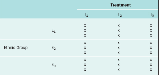
The RCBD is a generalization of the CRD whereby a second factor is included in the design so that the comparison of the levels of the treatment factor can be adjusted for its effects. For example, in the endometrial thickness study, there may be three different ethnic groups of women, E₁, E₂, and E₃, included in the study. Because the variation of the endometrial thicknesses may be higher between two different ethnic groups than within a given ethnic group, it would be wise to block on the ethnic group factor. In this case, we would randomly select 9 subjects from ethnic group E₁ and randomly assign 3 to each of the three treatments; likewise for ethnic groups E₂ and E₃, for a total of 27 subjects. The data layout would appear as in Table 9-2.

Table 9-2 Data Layout For a Randomized Complete Block Design

Latin Square Design (LSD)

To control for a second factor, a Latin square design is used. For example, the subjects in the endometrial thickness study come from three different age groups, A₁, A₂, and A₃. Because the endometrial thickness variable is likely to be more homogeneous for subjects from a given age group than for subjects from two different age groups, we should block on the age group in addition to the ethnic group.

Repeated Measures Design

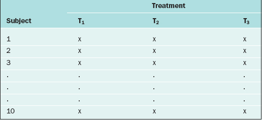
If in the RCBD the blocking factor is the subject, and the same subject is measured repeatedly, then the design becomes a repeated measures design. For instance, suppose that each of 10 subjects receives three different BP medications at different time points. For each medication, the BP is measured 5 days after the medication is started, then there is a 2-week “wash-out period” before starting the next medication. Also, the order of the medications is randomized. The data layout appears as in Table 9-3.

Table 9-3 Data Layout For a Repeated Measures Design

Many more sophisticated and complex experimental designs exist, and can be found in any standard text on experimental design.^4,⁵ For evaluating the validity, importance, and relevance of clinical trial results, see the article by The Practice Committee of the American Society for Reproductive Medicine.⁶ For surveys, there are many ways in which the sampling can be carried out (e.g., simple random sampling, stratified random sampling, cluster sampling, systematic sampling, or sequential sampling).^7,⁸

DESCRIPTIVE STATISTICAL METHODS

After the survey has been taken, the study has been carried out, or the experiment has been performed, then the data are obtained and entered into a spreadsheet or other usable form. After the data entry and data error checking have been completed, the first statistical analyses are performed; these are most often descriptive analyses—organizing and summarizing the data in the sample. Many different statistical methods are used to help organize and summarize the data. The descriptive statistical methods used for continuous variables differ from those used for discrete variables.

Continuous Variables

The principal descriptive features of continuous variables are (1) central location and (2) variability (or dispersion).

An important numerical measure of the centrality of a continuous variable is the mean:

where n = number of observations and x_i = i^th measurement in the sample.

Alternative measures of centrality are the median (middle measurement, or average of the two middle measurements if n is even, in the list of measurements rank-ordered from smallest to largest) and the mode (most frequent measurement).

A simple numerical measure of the variability or dispersion of a continuous variable is the range: the largest measurement minus the smallest measurement. The larger the variability in the measurements, the larger the range will be. A more common numerical measure of variability is the variance:

Note that the variance is approximately the average of the squared deviations (or distances) between each measurement and its mean. The more dispersed the measurements are, the larger s² is. Because s² is measured in the square of the units of the actual measurements, sometimes the standard deviation is used as the preferred measure of variability:

Also of interest for a continuous variable is its distribution (i.e., a representation of the frequency of each measurement or intervals of measurements). There are many forms for the graphical display of the distribution of a continuous variable, such as a stem-and-leaf plot, boxplot, or bar chart. From such a display, the central location, dispersion, and indication of “rare” measurements (low frequency) and “common” measurements (high frequency) can be identified visually.²

It is often of interest to know if two continuous variables are linearly related to one another. The Pearson correlation coefficient, r, is used to determine this. The values of r range from –1 to +1. If r is close to –1, then the two variables have a strong negative correlation (i.e., as the value of one variable goes up, the value of the other tends to go down [consider “number of years in practice after residency” and “risk of errors in surgery”]). If r is close to +1, then the two variables are positively correlated (e.g., “fetal humeral soft tissue thickness” and “gestational age”). If r is close to zero, then the two variables are not linearly related. One set of guidelines for interpreting r in medical studies is: |r| > 0.5 ⇒ “strong linear relationship,” 0.3< |r| ≤ 0.5⇒ “moderate linear relationship,” 0.1 < |r| ≤ 0.3⇒ “weak linear relationship,” and |r| ≤ 0.1⇒ “no linear relationship”.^9,¹⁰

Discrete Variables

For summarization of a discrete variable, a frequency table is used: for each discrete value of the variable, its frequency (how many times it occurs in the sample of, say, n observations) and relative frequency (frequency/n) are recorded. Of course, the sum of the frequencies over all of the discrete levels of the variable must be n, and the sum of the relative frequencies must be 1.0 (100%).

For two discrete variables the data are summarized in a contingency table. A two-way contingency table is a cross-classification of subjects according to the levels of each of the two discrete variables. An example of a contingency table is given in Table 9-4.

Table 9-4 Contingency Table for the Cross-classification of Subjects According to Treatment and Outcome.

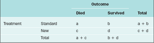
Here, there are a + b + c + d subjects in the sample; there are “a” subjects under the standard treatment who died, “b” subjects under the standard treatment who survived, and so on. If it is desired to know if two discrete variables are associated with one another, then a measure of association must be used. Which measure of association would be appropriate for a given situation depends on whether the variables are nominal or ordinal or a mixture.^11,¹²

In medical research, two of the important measures that characterize the relationship between two discrete variables are the risk ratio and the odds ratio. The risk of an event, p, is simply the probability or likelihood that the event occurs. The odds of an event is defined as p/(1–p) and is an alternative measure of how often an event occurs. The risk ratio (sometimes called relative risk) and odds ratio are simply ratios of the risks and odds, respectively, of an event for two different conditions. In terms of the contingency table given in Table 9-4, these terms are defined as follows.

Term	Definition
risk of death for those on the standard treatment	a/(a+b)
risk of death for those on the new treatment	c/(c+d)
odds of death for those on the standard treatment	a/b
odds of death for those on the new treatment	c/d
risk ratio of death	a(c+d)/c(a+b)
odds ratio of death	ad/bc

Note that a risk ratio of 4.0 means that the risk of death under the standard treatment is four times that under the new treatment. An odds ratio of 4.0 means that the odds of death are four times higher under the standard treatment than under the new treatment.

Another important measure in clinical practice is the risk difference, RD, the absolute difference between the risk of death under the standard treatment and the risk of death under the new treatment:

The inverse of the risk difference is the number needed to treat, NNT:

NNT is an estimate of how many subjects would need to receive the new treatment before there would be one more or less death, as compared to the standard treatment.

For example, in a study by Marcoux and colleagues ¹³ 341 women with endometriosis-associated subfertility were randomized into two groups, laparoscopic ablation and laparoscopy alone. The study outcome was “pregnancy > 20 weeks’ gestation.” Of the 172 women in the first group, 50 became pregnant; of the 169 women in the second group, 29 became pregnant (a = 50, b = 122, c = 29, and d = 140). The risk of pregnancy is 0.291 in the first group and 0.172 in the second group; the corresponding odds of pregnancy are 0.410 and 0.207. The risk ratio is 1.69 and the odds ratio is 1.98. The likelihood of pregnancy is 69% higher after ablation than after laparoscopy alone; the odds of pregnancy are about doubled after ablation compared to laparoscopy alone. The risk difference is

and number needed to treat is

Rounding upward, approximately 9 women must undergo ablation to achieve 1 additional pregnancy.

DIAGNOSTIC TEST EVALUATION

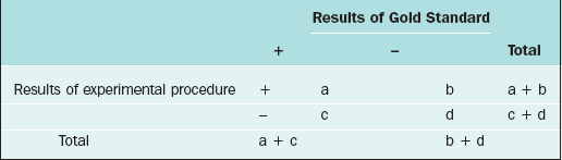
A specialized contingency table is formed when one factor represents the results of an accurate, standard test (sometimes called the Gold Standard), and the other factor represents the results of a new, perhaps less invasive, experimental procedure. This contingency table, used for diagnostic test evaluation, is given in Table 9-5.

Table 9-5 Contingency Table for Diagnostic Test Evaluation

Several different measures are used to assess the effectiveness of the experimental procedure relative to the Gold Standard; they are defined and interpreted below.

Term	Definition	Interpretation
prevalence rate	(a+c)/(a+b+c+d)	proportion of the sample that is truly positive
sensitivity	a/(a+c)	proportion of true positives who test positive with the experimental procedure
specificity	d/(b+d)	proportion of true negatives who test negative with the experimental procedure
positive predictive value	a/(a+b)	proportion of those testing positive with experimental procedure who are truly positive
negative predictive value	d/(c+d)	proportion of those testing negative with experimental procedure who are truly negative
false positives	b	number of subjects who are negative but test positive
false negatives	c	number of subjects who are positive but test negative

Use of these measures provides insight into the effectiveness of a new, experimental procedure relative to the Gold Standard.¹⁴^–¹⁶ To select that cutoff point for the experimental procedure that defines a “+” or “–” result in such a way that sensitivity and specificity are optimized, Receiver Operating Characteristic (ROC) curves are used.¹⁷ The ROC curve is a plot of the sensitivity of test (Y-axis) versus the false positive rate (X-axis; 1-specificity). This measure is used to assess how well a test can identify patients with a disease. An area under the curve of 1 is a perfect test and 0.5 is a useless test.

ESTIMATION

Generally, there are two ways in which inferences can be made to a population of interest: (1) estimate population parameters or (2) test hypotheses about population parameters.

A point estimate of a parameter, calculated from a random sample of the population, is the best single estimated value of the parameter. If a random sample of 50 fetuses at 20 weeks’ gestation are each measured sonographically for fetal HSTT, and the average of these 50 values is 9.7 mm, then our point estimate of the true mean fetal HSTT (i.e., the mean fetal HSTT of all such fetuses) is 9.7 mm.

Confidence Intervals

Although the point estimate is expected to be “close” to the parameter value, we are often interested in how close it is. Therefore, many researchers prefer to use a confidence interval to estimate the parameter. A confidence interval is an interval for which the endpoints are determined by statistics calculated from the sample; for this interval there is a high probability (usually set at 95%) that it contains the population parameter value. For most applications, the point estimate is at the midpoint of the confidence interval. In the example above, if the 95% confidence interval for the mean fetal HSTT is [7.2, 12.2], then we say that we are 95% confident that the true mean fetal HSTT falls between 7.2 mm and 12.2 mm. This interval can also be written as 9.7 mm ± 2.5 mm. The value 2.5 is called the margin of error; it represents the range of values on either side of the point estimate, 9.7 mm, that are regarded as “plausible” values of the true mean fetal HSTT. Values farther than 2.5 mm away from the point estimate are regarded as “implausible” values. In this way, the confidence interval, with its margin of error, provides a measure of the reliability of the point estimate.

Confidence intervals that have a small width (i.e., small margin of error) are desirable because the true value is then estimated reliably, or within a small range of values. One way to reduce the width of a confidence interval is to increase the sample size. For example, the formula for the 95% confidence interval of a population mean is

This particular formula is valid for relatively large samples, say n ≥30. Note that the margin of error is

which decreases when n increases.

The basic formula for most confidence intervals is

where the reliability coefficient is a percentile taken from an appropriate distribution, and the standard error is the standard deviation of the estimator. In the confidence interval for a population mean given above, the point estimator is the sample mean,

the reliability coefficient is the 97.5th percentile from the standard normal distribution, and the standard error is

Refer to any standard statistics text to obtain confidence interval formulas for population parameters (e.g., McClave and Sincich²).

TESTS OF HYPOTHESES

For statistical purposes, research questions are framed in terms of two hypotheses. The null hypothesis, H₀, is typically the hypothesis of “no change,” or “no difference,” or the status quo, and is stated in terms of parameters. The alternative hypothesis, also called the research hypothesis, H_A, is typically the hypothesis of “change” and is the complement of H₀. For example, consider the research hypothesis: “the mean fetal HSTT at 20 weeks’ gestation is less than 10 mm.” The hypotheses would be written formally as:

where μ = mean fetal HSTT.

P-Value

A statistical test of hypothesis is a procedure whereby a determination is made as to whether there is sufficiently strong evidence in the data to support the research hypothesis, H_A. If so, then H₀ is “rejected”; otherwise H₀ is “not rejected.” How is this determination made? A quantity called the P-value (P) is calculated from the data. The P-value is actually a probability and hence lies between zero and one. Small values of P correspond to a rejection of H₀. In this case, the test result is said to be “statistically significant.” How small does P have to be to lead to a rejection of H₀? Most researchers use a cutoff (called the level of significance of the test) of 0.05. That is, if P < 0.05, then H₀ is rejected, and one can conclude that there is strong evidence in the data to support the research hypothesis, H_A, at the 0.05 level of significance. When P ≥ 0.05, then H₀ is not rejected and one concludes that there is not sufficient evidence in the data to support the research hypothesis. For most research studies, the P-value for a given result is simply reported, leaving the reader to make his/her own conclusion about the strength of evidence in the data supporting the research hypothesis.

The P-value represents the probability of obtaining the sample that was observed “by chance alone” (i.e., the probability of obtaining a sample at least as contradictory to H₀ as the one observed when H₀ is assumed to be true). So, if P is very small, then it implies that the observed sample is very rare if H₀ is really true, leading to the conclusion that H₀ must not be true. If one test has P = 0.10 and a second test has P = 0.01, then the evidence against H₀ is 10 times stronger in the second test than in the first test in the sense that the probability of obtaining a sample at least as contradictory to H₀ as the observed sample is 10 times higher in the first test than in the second test. That is, the sample in the first test is not as extreme when H₀ is true as the sample in the second test.

Type I and II Errors, Statistical Power

When making the decision about whether the evidence in the data is strong enough to reject H₀, the only two possible outcomes are (1) reject H₀ or (2) fail to reject H₀. In this decision-making process, there are only two possible errors that can be made: (1) incorrectly reject H₀ (i.e., reject H₀ even though H₀ is true), or (2) incorrectly fail to reject H₀ (i.e, fail to reject H₀ even though H₀ is false). The first error is called the type I error and its probability of occurring is denoted by alpha (α). The second error is called the type II error and its probability of occurring is denoted by beta (β).

In practice we would like both α and β to be small. The statistical test that is used to make the decision about rejecting or failing to reject H₀ is designed to ensure that α is no larger than the level of significance chosen by the researcher (again, 0.05 is the most common choice for the level of significance). Hence, when testing a set of hypotheses one can be confident that the likelihood of incorrectly rejecting H₀ is at most, say, 0.05. The type II error rate, β, is controlled by, among other things, the sample size, n. That is, the larger n is, the lower β is.

Statistical power is defined as 1 – β, which is the probability of correctly rejecting H₀ (i.e., rejecting H₀ when H₀ is really false). In practice, we would like the statistical power to be high (at least 0.8) for those alternatives (i.e., values of the parameter in H_A) that are deemed to be clinically important. As indicated above, β decreases as n increases, and hence power increases with n.

STATISTICAL PROCEDURES

Comparison of Means

When the means of k ≥ 2 populations are compared, then the one-way analysis of variance (ANOVA) is used for the analysis; it is based on k-independent samples and the corresponding design is the CRD. The hypotheses being tested are:

For example, one may be interested in comparing the mean fetal HSTT among four ethnic groups of women: white, African-American, Asian, and “other.” If H₀ is rejected (e.g., P < 0.05), then it is concluded that the mean fetal HSTT is not the same for all four ethnic groups. The determination of how the four means differ from one another is made through a multiple comparisons procedure. There are many such procedures, but the recommended ones are Tukey’s HSD (“honestly significant difference”) post hoc test, the Bonferroni-Dunn post hoc test, or the Neuman-Keuls test.¹⁸ In the special case of the ANOVA in which k = 2, so that the means of two populations are compared based on two independent samples, the statistical test is called the two-sample (or pooled-sample) t-test.

If the k samples are not independent, but rather matched (i.e., correlated), then an ANOVA based on the RCBD is conducted. In the special case where k = 2, so that the means of two populations are compared based on paired samples, then the statistical test is called the paired t-test. For instance, if the fetal HSTT for each of n subjects is measured at 20 weeks’ gestation and again at 30 weeks’ gestation, then the two observations are correlated because they come from the same subject. In this case, the P-value is based on the paired differences of the two measurements. If we wish to test that the mean fetal HSTT is higher at 30 weeks than at 20 weeks, the hypotheses would be written

where μ represents the mean fetal HSTT.

What is an appropriate sample size to use for a two-sample t-test or a paired t-test? If the two populations have comparable standard deviations, then a sample of size at least n = (16)(s_c/δ)² for each group will ensure 80% power for the two-sample t-test conducted at the 0.05 level of significance, where s_c is the estimate of the common standard deviation of the two samples, and δ is a mean difference that is deemed to be clinically important.¹⁹ For a paired-sample t-test, a sample of size at least n = (8)(s_d/δ)² pairs will ensure 80% power for a 0.05 level test, where s_d is the standard deviation of the differences of the paired measurements.¹⁹

If means are compared among the levels of each of two factors, then a two-way ANOVA is conducted. Consider comparing the mean fetal HSTT between two age groups and among four ethnic groups of pregnant women. In addition to the two effects, age and ethnic group, there is a third effect to consider—the statistical interaction between age and ethnic group. A two-factor statistical interaction exists if, for instance, the difference in mean fetal HSTT between “young” and “old” pregnant women is not the same for every ethnic group. For example, African-American young and old women may have fetuses that differ widely in mean HSTT, whereas Asian young and old women may have fetuses with comparable mean HSTT levels.

In general, a design with N factors is analyzed using an N-way ANOVA, where 2-factor interactions, 3-factor interactions, …, and the N-factor interaction may be analyzed.

STUDYING RELATIONSHIPS/PREDICTION

Often in medical research one is interested in studying the effects of a set of independent variables, X₁, X₂, …, X_k, on a continuous dependent variable, Y. Alternatively, one may be interested in predicting Y from a set of predictor variables. This can be done using a multiple regression analysis. Such an analysis models the mean, or expected, Y value, E(Y), on a multiple linear function of the independent (or predictor) variables:

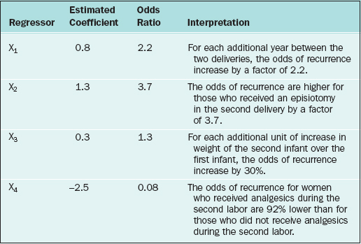
A major result of the multiple regression analysis is the estimation of the regression coefficients β_i = 1, 2, …, k, and the statistical test of significance for each coefficient. The hypotheses being tested are:

for i = 1, 2, …, k.

A regression coefficient β_i is interpreted as the amount by which E(Y) changes for a unit increase in x_i while all other predictor variables are held constant. Suppose we regress a pregnant woman’s body temperature on (1) number of days gestation, (2) age, (3) ethnic group (where 1=white and 0=other), and (4) BMI. Notationally, we would write

There are two cautionary notes concerning the predictor variables in any regression model, including logistic and Cox regression models:

(1) Each predictor variable is only allowed to be continuous or binary. If a predictor variable is discrete with k > 2 levels, then k – 1 “dummy” or “indicator” variables must be formed to represent the k-level discrete variable in the regression equation.

(2) The predictor variables in a regression model should not be highly correlated with each other. For instance, a correlation coefficient between any two predictors exceeding 0.8 or 0.9 in absolute value would lead to a condition called multicollinearity, which leads to severe instability of the estimated regression coefficients. See any standard regression text for further discussion of these two points.²⁰^–²³

What is an appropriate sample size for a multiple regression? In general, a sample size of at least n = 10k should be used,²² where k is the number of predictors in the model. However, this guarantees nothing about the statistical power. To ensure 80% power of detecting a “medium” size effect, the sample size should be at least n = 50 + 8k.²⁴

COMPARING PROPORTIONS

Consider the comparison of two population proportions,

As an example, suppose we wish to compare the proportion of neonates with fetal growth restriction (FGR) between urban and rural first-time mothers.

Suppose that in samples of 100 urban and 100 rural first-time mothers, 12 urban mothers and 15 rural mothers had babies with FGR. For these data, the P-value associated with the above hypotheses is P = 0.535; there is not strong evidence that the two proportions are different.

As a generalization, consider the regression of a discrete variable on a set of predictor variables. The logistic regression equation is used in this case; if p represents a probability of interest (e.g., probability of FGR), then the logistic regression equation is:

The quantity p/(1–p) is the odds of the event of interest (i.e., occurrence of FGR), and the left side of the equation, log(p/(1–p)), is called the logit of the event of interest. So, β_i represents the amount by which the logit changes for a unit increase in x_i, and e^βi respresents the odds ratio (i.e., the ratio of the odds of the event of interest associated with a unit increase in x_i).

As an example, an obstetrics and gynecology resident from the Wright State University School of Medicine wished to identify the predictors of the recurrence of third- and fourth-degree obstetrical lacerations for women who had given birth to two children. A retrospective chart review of vaginal births at Miami Valley Hospital in Dayton, Ohio was conducted. The outcome is “recurrence of third- and fourth-degree obstetrical lacerations” (coding: 0=No, 1=Yes), and the predictors were: X₁ = number of years between the two deliveries, X₂ = whether an episiotomy was performed in the second delivery (coding: 0=No, 1=Yes), X₃ = birthweight of second infant minus birthweight of first infant, and X₄ = whether analgesics were received during the second labor (coding: 0=No, 1=Yes). The data were analyzed by the Wright State University Statistical Consulting Center. The logit of recurrence of third- and fourth-degree obstetrical lacerations was regressed on the four predictors for a sample of 1852 women. The estimated model is:

Each of the coefficients is statistically significant at the 0.05 level of significance. The results of the analysis are given below.

What is an appropriate sample size for a logistic regression? Consider a binary outcome variable. In general, the number of subjects falling into the smaller of the two outcome levels should be at least 10k, where k = number of predictor variables in the logistic regression equation.²⁵^–²⁷ To ensure a specified power, a sample size software or a table²⁸ must be used.

COMPARING SURVIVAL RATES

In survival studies, one is typically interested in the occurrence of a particular event over time (e.g., death). It is common to observe subjects from a well-defined starting point and to establish an ending time of the study, which may be days, or weeks, or …, years later. During this follow-up period, one of three things will happen for a given subject: (1) the event of interest will occur before the end of follow-up, (2) the subject will fall out of the study (e.g., move away, die from a cause having nothing to do with the event under study, or refuse to participate in the study any further), or (3) the subject is observed through the entire follow-up period without experiencing the event of interest. In the latter two cases, the observations are said to be censored (i.e., incomplete information is available for these subjects). For instance, in the case of death, all that is known about the subject who survives the entire follow-up period without dying is that he or she dies at some time after the end of follow-up. In the former case, complete information is available (i.e., the “survival” time until the event occurs is known), so the observation is not censored.

Two important quantities for evaluating survival data are (1) the survival function and (2) the hazard function. The survival function, S(t), is the probability that a subject experiences the event of interest after time t; S(t) = P[X>t], where X represents the time until the event of interest occurs. The estimated values of S(t) plotted against t are called Kaplan-Meier curves.²⁹

The hazard function is, mathematically,

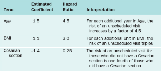
Practically, it is interpreted as the average number of times the event of interest occurs in one unit of time at time t. If the event of interest is, say, death, then an increasing hazard function corresponds to an increased death rate. The hazard ratio is the ratio of two hazard functions.

The standard statistical model for analyzing survival data is the Cox proportional hazards regression model.³⁰ In this model the hazard rate is regressed on a set of regressor variables,

where h₀(t) is an arbitrary baseline hazard rate. This model is used to study the effects of the regressor variables on the hazard function. Suppose that 1000 new mothers are monitored from delivery to the baby’s first unscheduled hospital visit. The study period lasts 2 years, and new deliveries are enrolled during the first year. The hazard function (for baby’s first unscheduled hospital visit) is regressed on mother’s age, mother’s BMI, and whether the mother delivered by cesarean section (coding: 1=Yes, 2=No). In the table below, the results are presented along with the interpretation. Assume that all of the β-coefficients are statistically significant.