CHAPTER 22 Risk Calculation
One of the most important aspects of genetic counseling is the provision of a risk figure. This is often referred to as a recurrence risk. Estimation of the recurrence risk usually requires careful consideration and takes into account:
Probability Theory
Bayes’ Theorem
The initial probability of each event is known as its prior probability, and is based on ancestral or anterior information. The observations that modify these prior probabilities allow conditional probabilities to be determined. In genetic counseling these are usually based on numbers of offspring and/or the results of tests. This is posterior information. The resulting probability for each event or outcome is known as its joint probability. The final probability for each event is known as its posterior or relative probability and is obtained by dividing the joint probability for that event by the sum of all the joint probabilities.
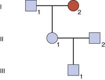
This is not an easy concept to grasp! To try to make it a little more comprehensible, consider a pedigree with two males, I3 and II1, who have a sex-linked recessive disorder (Figure 22.1). The sister, II2, of one of these men wishes to know the probability that she is a carrier. Her mother, I2, must be a carrier because she has both an affected brother and an affected son (i.e., she is an obligate carrier). Therefore, the prior probability that II2 is a carrier equals 1/2. Similarly, the prior probability that II2 is not a carrier equals 1/2.
This information is now incorporated into a bayesian calculation (Table 22.1). From this table, the posterior probability that II2 is a carrier equals 1/16/(1/16 + 1/2), which reduces to 1/9. Similarly the posterior probability that II2 is not a carrier equals 1/2/(1/16 + 1/2), which reduces to 8/9. Another way to obtain these results is to consider that the odds for II2 being a carrier versus not being a carrier are 1/16 to 1/2 (i.e., 1 to 8, which equals 1 in 9). Thus, by taking into account the fact that II2 has three healthy sons, we have been able to reduce her risk of being a carrier from 1 in 2 to 1 in 9.
| Probability | II2 is a Carrier | II2 is not a Carrier |
|---|---|---|
| Prior | 1/2 | 1/2 |
| Conditional | ||
| Three healthy sons | (1/2)3 = 1/8 | (1)3 = 1 |
| Joint | 1/6 | 1/2 (= 8/16) |
| Expressed as odds | 1 to | 8 |
| Posterior | 1/9 | 8/9 |
Autosomal Dominant Inheritance
Reduced Penetrance
For a condition showing reduced penetrance, the risk that the child of an affected individual will be affected equals 1/2—i.e., the probability that the child will inherit the mutant allele, × P, the proportion of heterozygotes who are affected. Therefore, for a disorder such as hereditary retinoblastoma, an embryonic eye tumor (p. 215), which shows dominant inheritance in some families with a penetrance of P = 0.8, the risk that the child of an affected parent will develop a tumor equals 1/2 × 0.8, which equals 0.4.
A more difficult calculation arises when a risk is sought for the future child of someone who is healthy but whose parent has, or had, an autosomal dominant disorder showing reduced penetrance (Figure 22.2).
| Probability | II1 Is Heterozygous | II1 Is Not Heterozygous |
|---|---|---|
| Prior | 1/2 | 1/2 |
| Conditional | ||
| Not affected | 1 − P | 1 |
| Joint | 1/2 (1 − P) | 1/2 |
Delayed Age of Onset
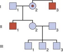
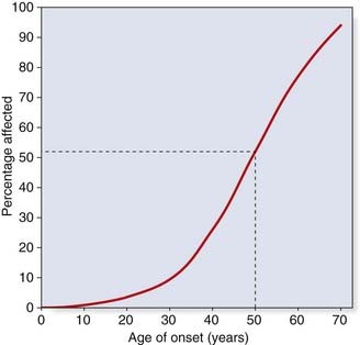
Consider someone who has died with a confirmed diagnosis of Huntington disease (Figure 22.4). This is a late-onset autosomal dominant disorder. The son of I2 is entirely healthy at age 50 years and wishes to know the probability that his 10-year-old daughter, III1, will develop Huntington disease in later life. In this condition, the first signs usually appear between the ages of 30 and 60 years, and approximately 50% of all heterozygotes have shown signs by the age of 50 years (Figure 22.5).
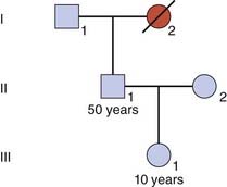
To answer the question about the risk to III1, it is first necessary to calculate the risk for II1 (if III1 was asking about her own risk, her father might be referred to as the dummy consultand). The probability that II1 has inherited the gene, given that he shows no signs of the condition, can be determined by a simple bayesian calculation (Table 22.3).
| Probability | II1 Is Heterozygous | II1 Is Not Heterozygous |
|---|---|---|
| Prior | 1/2 | 1/2 |
| Conditional | ||
| Unaffected at age 50 years | 1/2 | 1 |
| Joint | 1/4 | 1/2 |
Autosomal Recessive Inheritance
With an autosomal recessive condition, the biological parents of an affected child are both heterozygotes. Apart from undisclosed non-paternity and donor insemination, there are two possible exceptions, both of which are very rare. These arise when only one parent is a heterozygote, in which case a child can be affected if either a new mutation occurs on the gamete inherited from the other parent, or uniparental disomy occurs resulting in the child inheriting two copies of the heterozygous parent’s mutant allele (p. 113). For practical purposes, it is usually assumed that both parents of an affected child are carriers.
Carrier Risks for the Extended Family
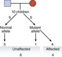
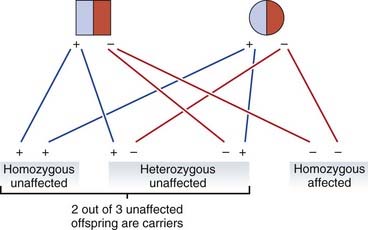
When both parents are heterozygotes, the risk that each of their children will be affected is 1 in 4. On average three of their four children will be unaffected, of whom, on average, two will be carriers (Figure 22.6). Therefore the probability that the healthy sibling of someone with an autosomal recessive disorder will be a carrier equals 2/3. Carrier risks can be derived for other family members, starting with the assumption that both parents of an affected child are carriers (Figure 22.7).
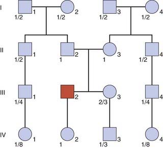
When calculating risks in autosomal recessive inheritance the underlying principle is to establish the probability that each prospective parent is a carrier, and then multiply the product of these probabilities by 1/4, this being the risk that any child born to two carriers will be affected. Therefore, in Figure 22.7, if the sister, III3, of the affected boy was to marry her first cousin, III4, the probability that their first baby would be affected would equal 2/3 × 1/4 × 1/4—i.e., the probability that III3 is a carrier times the probability that III4 is a carrier times the probability that a child of two carriers will be affected. This gives a total risk of 1/24.
If this same sister, III3, was to marry a healthy unrelated individual, the probability that their first child would be affected would equal 2/3 × 2pq × 1/4—i.e., the probability that III3 is a carrier times the carrier frequency in the general population (p. 132) times the probability that a child of two carriers will be affected. For a condition such as cystic fibrosis, with a disease incidence of approximately 1 in 5000, q2 = 1/2500 and therefore q = 1/50 and thus 2pq = 1/25. Therefore the final risk would be 2/3 × 1/25 × 1/4, or 1 in 150.
Modifying a Carrier Risk by Mutation Analysis
Population screening for cystic fibrosis has been introduced in the United Kingdom after pilot studies (p. 321). More than 1500 different mutations have been identified in the cystic fibrosis gene, so that carrier detection by DNA mutation analysis is not straightforward. However, a relatively simple test has been developed for the most common mutations, which enables about 90% of all carriers of western European origin to be detected. What is the probability that a healthy individual who has no family history of cystic fibrosis, and who tests negative on the common mutation screen, is a carrier?
The answer is obtained, once again, by drawing up a simple bayesian table (Table 22.4). The prior probability that this healthy member of the general population is a carrier equals 1/25; therefore the prior probability that he or she is not a carrier equals 24/25. If this individual is a carrier, then the probability that the common mutation test will be normal is 0.10 as only 10% of carriers do not have a common mutation. The probability that someone who is not a carrier will have a normal common mutation test result is 1.
Table 22.4 Bayesian Table for Cystic Fibrosis Carrier Risk if Common Mutation Screen Is Negative
| Probability | Carrier | Not a Carrier |
|---|---|---|
| Prior | 1/25 | 24/25 |
| Conditional | ||
| Normal result on common mutation screening | 0.10 | 1 |
| Joint | 1/250 | 24/25 |
Sex-Linked Recessive Inheritance
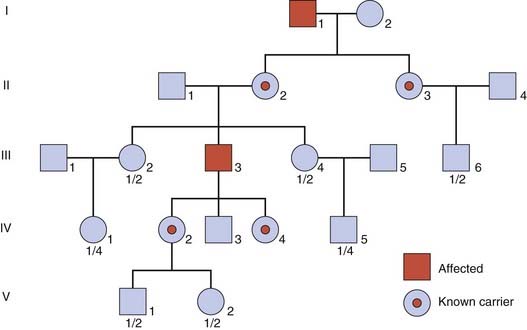
This pattern of inheritance tends to generate the most complicated risk calculations when counseling for mendelian disorders. In severe sex-linked conditions, affected males are often unable to have their own children. Consequently, these conditions are usually transmitted only by healthy female carriers. The carrier of a sex-linked recessive disorder transmits the gene on average to half of her daughters, who are therefore carriers, and to half of her sons who will thus be affected. If an affected male does have children, he will transmit his Y chromosome to all of his sons, who will be unaffected, and his X chromosome to all of his daughters, who will be carriers (Figure 22.8).
An example of how the birth of unaffected sons to a possible carrier of a sex-linked disorder results in a reduction of her carrier risk has already been discussed in the introductory section on Bayes’ theorem (p. 339). In this section, we consider two further factors that can complicate risk calculation in sex-linked recessive disorders.
The Isolated Case
In practice it is often very difficult to distinguish among these three possibilities unless reliable tests are available for carrier detection. If a woman is found to be a carrier, then risk calculation is straightforward. If the tests indicate that she is not a carrier, the recurrence risk is probably low, but not negligible because of the possibility of gonadal mosaicism.
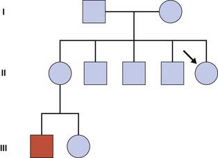
Leaving aside the complicating factor of gonadal mosaicism, risk calculation in the context of an isolated case (Figure 22.9) is possible, but may require calculation of the risk for a dummy consultand within the pedigree as well as taking account of the mutation rate, or µ. For a fuller understanding of µ, the student is referred to one of the more detailed texts listed at the end of the chapter.
Incorporating Carrier Test Results
For example, in DMD, the serum creatine kinase level is raised in approximately two out of three obligate carriers (see Figure 20.1; p. 314). Therefore, if a possible carrier such as II2 in Figure 22.1 is found to have a normal level of creatine kinase, this would provide further support for her not being a carrier. The test result therefore provides a conditional probability, which is included in a new bayesian calculation (Table 22.5).
| Probability | II2 Is a Carrier | II2 Is Not a Carrier |
|---|---|---|
| Prior | 1/2 | 1/2 |
| Conditional | ||
| Three healthy sons | 1/8 | 1 |
| Normal creatine kinase | 1/3 | 1 |
| Joint | 1/48 | 1/2 |
The Use of Linked Markers
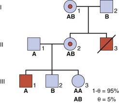
For many single-gene disorders the genomic location is known and sequence analysis possible. Linked DNA markers are therefore used less often today than formerly but still sometimes have a role in clarifying the genetic status of an individual in a pedigree, providing there is certainty that the disease in question is caused by mutations at one particular gene locus (i.e., the disease is not genetically heterogeneous). Take the example of DMD (p. 307), in which each family usually has its own unique mutation. If there are no surviving affected males, linked markers may be employed to help determine carrier detection.
As an illustration, consider the sister of a boy affected with DMD, whose mother is an obligate carrier as she herself had an affected brother (Figure 22.10). A DNA marker with alleles A and B is available and is known to be closely linked to the DMD disease locus with a recombination fraction (θ) equal to 0.05. The disease allele must be in coupling with the A marker allele in II2 as this woman has inherited both the A allele and the DMD allele on the X chromosome from her mother (she must have inherited the B allele from her father, so the A allele must have come from her mother). Therefore, if III3 inherits this A allele from her mother, the probability that she will also inherit the disease allele and be a carrier equals 1 − θ—i.e., the probability that a crossover will not have occurred between the disease and marker loci in the meiosis of the ova that resulted in her conception. For a value of θ equal to 0.05, this gives a carrier risk of 0.95 or 95%. Similarly, the probability that III3 will be a carrier if she inherits the B allele from her mother equals 0.05 or 5%.
Bayes’ Theorem and Prenatal Screening
As a further illustration of the potential value of Bayes’ theorem in risk calculation and genetic counseling, an example from prenatal screening is given. Consider the situation that arises when a woman age 20 years presents at 13 weeks’ gestation with a fetus that has been shown on ultrasonography to have significant nuchal translucency (NT) (see Figure 21.5). NT may be present in about 75% of fetuses with Down syndrome (p. 327). In contrast, the incidence in babies not affected with Down syndrome is approximately 5%. In other words, NT is 15 times more common in Down syndrome than in unaffected babies.
Actual values for these prior probabilities can be obtained by reference to a table showing maternal age-specific risks for Down syndrome (see Table 18.4; p. 274). For a woman age 20 years, the incidence of Down syndrome is approximately 1 in 1500; hence, the prior probability that the baby will be unaffected equals 1499/1500. If these prior probability values are used in a bayesian calculation, it can be shown that the posterior probability risk that the unborn baby will have Down syndrome is approximately 1 in 100 (Table 22.6). Obviously, this is much lower than the conditional odds of 15 to 1 in favor of the baby being affected.
Table 22.6 Bayesian Calculation to Show the Posterior Probability that a Fetus with Nuchal Translucency Conceived by a 20-Year-Old Mother Will Have Down Syndrome
| Probability | Fetus Unaffected | Fetus Affected |
|---|---|---|
| Prior | 1499/1500 | 1/1500 |
| Conditional | ||
| Nuchal translucency | 1 | 15 |
| Joint | 1499/1500 = 1 | 1/100 |
| Expressed as odds | 100 to | 1 |
| Posterior | 100/101 | 1/101 |
In practice, the demonstration of NT on ultrasonography in a fetus would usually prompt an offer of definitive chromosome analysis by placental biopsy, amniocentesis, or fetal blood sampling (see Chapter 21). This example of NT has been used to emphasize that an observed conditional probability ratio should always be combined with prior probability information to obtain a correct indication of the actual risk.
Empiric Risks
Multifactorial Disorders
One of the basic principles of multifactorial inheritance is that the risk of recurrence in first-degree relatives, siblings and offspring, equals the square root of the incidence of the disease in the general population (p. 146)—i.e.,  , where P equals the general population incidence. For example, if the general population incidence equals 1/1000, then the theoretical risk to a first-degree relative equals the square root of 1/1000, which approximates to 1 in 32 or 3%. The theoretical risks for second- and third-degree relatives can be shown to approximate to
  and
and  , respectively. Therefore, if there is strong support for multifactorial inheritance, it is reasonable to use these theoretical risks when counseling close family relatives.
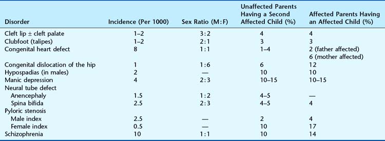
However, when using this approach it is important to remember that the confirmation of multifactorial inheritance will often have been based on the study of observed recurrence risks. Consequently, it is generally more appropriate to refer back to the original family studies and counsel on the basis of the risks derived in these (Table 22.7).
Conditions Showing Causal Heterogeneity
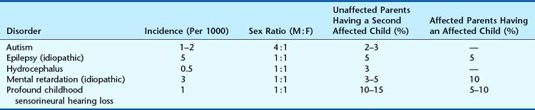
Many referrals to genetic clinics relate to a clinical phenotype rather than to a precise underlying diagnosis (Table 22.8). In these situations, great care must be taken to ensure that all appropriate diagnostic investigations have been undertaken before resorting to the use of empiric risk data (p. 346).
Bayes T. An essay towards solving a problem in the doctrine of chances. Biometrika. 1958;45:296-315.
Emery AEH. Methodology in medical genetics, 2nd edn. Edinburgh, UK: Churchill Livingstone; 1986.
An introduction to statistical methods of analysis in human and medical genetics.
Murphy EA, Chase GA. Principles of genetic counseling. Chicago: Year Book Medical; 1975.
A very thorough explanation of the use of Bayes’ theorem in genetic counseling.
Young ID. Introduction to risk calculation in genetic counselling, 2nd edn. Oxford, UK: Oxford University Press; 1999.
Elements