The viscosity of a fluid may be described simply as its resistance to flow or movement. Thus water, which is easier to stir than syrup, is said to have the lower viscosity. The reciprocal of viscosity is fluidity. Rheology (a term invented by Bingham and formally adopted in 1929) may be defined as the study of the flow and deformation properties of matter.

Historically the importance of rheology in pharmacy was merely as a means of characterizing and classifying fluids and semi-solids. For example, all pharmacopoeias have included a viscosity standard to control substances such as liquid paraffin. However, the increased reliance on in vitro testing of dosage forms as a means of evaluating their suitability for the grant of a marketing authorization and the increased use of polymers in formulations and the construction of devices has given added importance to measurement of flow properties. Furthermore, advances in the methods of evaluation of the viscoelastic properties of semi-solid materials has increased not only the amount and quality of the information that can be gathered but has also accelerated the time taken for its acquisition.

A proper understanding of the rheological properties of pharmaceutical materials is essential to the preparation, development, evaluation and performance of pharmaceutical dosage forms. This chapter describes rheological behaviour and techniques of measurement and will form a basis for the applied studies described in later chapters.

Newtonian fluids

Viscosity coefficients for Newtonian fluids

Dynamic viscosity

The definition of viscosity was put on a quantitative basis by Newton. He was the first to realize that the rate of flow (γ) was directly related to the applied stress (σ): the constant of proportionality is the coefficient of dynamic viscosity (η), more usually referred to simply as the viscosity. Simple fluids which obey this relationship are referred to as Newtonian fluids and those which do not are known as non-Newtonian.

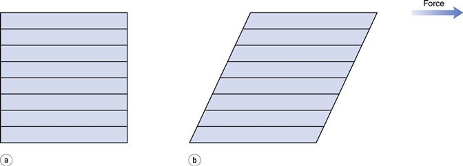
The phenomenon of viscosity is best understood by a consideration of a hypothetical cube of fluid made up of infinitely thin layers (laminae) which are able to slide over one another like playing cards in a pack or deck (Fig. 6.1a). When a tangential force is applied to the uppermost layer, it is assumed that each subsequent layer will move at progressively decreasing velocity and that the bottom layer will be stationary (Fig. 6.1b). A velocity gradient will therefore exist and this will be equal to the velocity of the upper layer in m s⁻¹ divided by the height of the cube in metres. The resultant gradient, which is effectively the rate of flow but is usually referred to as the rate of shear, γ, will have units of reciprocal seconds (s⁻¹). The applied stress, known as the shear stress, σ, is derived by dividing the applied force by the area of the upper layer and will thus have units of N m⁻².

Fig. 6.1 Representation of the effect of shearing a ‘block’ of fluid.

As Newton’s Law can be expressed as:

(6.1)

then

(6.2)

and η will have units of N m⁻²s. Thus, by reference to Equation 6.1, it can be seen that a Newtonian fluid of viscosity 1 N m⁻²s would produce a velocity of 1 m s⁻¹ for a cube of 1 m dimensions with an applied force of 1 N. Because the derived unit of force per unit area in the SI system is the pascal (Pa), viscosity should be referred to in Pa s or mPa s (the dynamic viscosity of water is approximately 1 mPa s). The centipoise (cP) and poise (1 P = 1 dyn cm⁻²s) were units of viscosity in the now redundant cgs system. These are no longer official and therefore are not recommended but are still relatively commonly used.

The values of the viscosity of water and some examples of other fluids of pharmaceutical interest are given in Table 6.1. Since viscosity is inversely related to temperature, in this case the values given are those measured at 20 °C.

Table 6.1

Viscosities of some fluids of pharmaceutical interest

Fluid	Dynamic viscosity at 20 °C (mPa s)
Chloroform	0.58
Water	1.002
Ethanol	1.20
Fractionated coconut oil	30.0
Glyceryl trinitrate	36.0
Propylene glycol	58.1
Soya bean oil	69.3
Rape oil	163
Glycerol	1490

Kinematic viscosity

The dynamic viscosity is not the only coefficient that can be used to characterize a fluid. The kinematic viscosity (ν) is also used and may be defined as the dynamic viscosity divided by the density of the fluid (ρ):

(6.3)

and the SI units will be m² s⁻¹ or, more usefully, mm² s⁻¹. The cgs unit was the Stoke (S = 10⁻⁴ m² s^-1) which together with the centiStoke (cS) may still be found in the literature.

Relative and specific viscosities

The viscosity ratio or relative viscosity (η_r) of a solution is the ratio of the viscosity of the solution to the viscosity of its solvent (η_o):

(6.4)

and the specific viscosity (η_sp) is given by:

(6.5)

In these calculations the solvent can be of any nature, although in pharmaceutical products it is most usually water.

For a colloidal dispersion, the equation derived by Einstein may be used.

(6.6)

where ϕ is the volume fraction of the colloidal phase (the volume of the dispersed phase divided by the total volume of the dispersion). The Einstein equation may be rewritten as:

(6.7)

when from Equation 6.4 it can be seen that as the left-hand side of Equation 6.7 is equal to the relative viscosity it can be rewritten as:

(6.8)

where the left-hand side equals the specific viscosity. Equation 6.8 can be rearranged to produce:

(6.9)

and as the volume fraction will be directly related to concentration, C, Equation 6.9 can be rewritten as:

(6.10)

where k is a constant.

When the dispersed phase is a high molecular mass polymer then a colloidal solution will result and, provided moderate concentrations are used, Equation 6.10 can be expressed as a power series:

(6.11)

Intrinsic viscosity

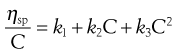
If η_sp/C, the viscosity number or reduced viscosity, is determined at a range of polymer concentrations (g dL⁻¹) and plotted as a function of concentration (Fig. 6.2), a linear relationship should be obtained. The intercept produced on extrapolation of the line to the ordinate will yield the constant k₁ which is referred to as the limiting viscosity number or the intrinsic viscosity, [η].

Fig. 6.2 Plot of concentration (g dL⁻¹) against reduced viscosity (η_sp/C), which by extrapolation gives the limiting viscosity number or intrinsic viscosity ([η]).

The limiting viscosity number may be used to determine the approximate molecular mass (M) of polymers using the Mark–Houwink equation:

(6.12)

where K and α are constants that must be obtained at a given temperature for the specific polymer–solvent system using other techniques such as osmometry or light scattering. However, once these constants have been determined, then viscosity measurements provide a quick and precise method of molecular mass determination of pharmaceutical polymers such as dextrans, which are used as plasma extenders. Also, the values of the two constants provide an indication of the shape of the molecule in solution: spherical molecules yield values of α = 0, whereas extended rods have values greater than 1.0. A randomly coiled molecule will yield an intermediate value (≈0.5).

The specific viscosity may be used in the following equation to determine the volume of a molecule in solution:

(6.13)

where C is concentration, N is Avogadro’s number, V is the hydrodynamic volume of each molecule and M is the molecular mass. However, it does suffer from the obvious disadvantage that the assumption is made that all polymeric molecules form spheres in solution.

Huggins’ constant

Finally, the constant k₂ in Equation 6.11 is referred to as Huggins’ constant and is equal to the slope of the plot shown in Figure 6.2. Its value gives an indication of the interaction between the polymer molecule and the solvent, such that a positive slope is produced for a polymer that interacts weakly with the solvent, and the slope becomes less positive as the interaction increases. A change in the value of Huggins’ constant can be used to evaluate the interaction of drug molecules in solution with polymers.

Boundary layers

From Figure 6.1 it can be seen that the rate of flow of a fluid over an even surface will be dependent upon the distance from that surface. The velocity, which will be almost zero at the surface, increases with increasing distance from the surface until the bulk of the fluid is reached and the velocity becomes constant. The region over which differences in velocity are observed is referred to as the boundary layer which arises because the intermolecular forces between the liquid molecules and those of the surface result in a reduction of movement of the layer adjacent to the wall to zero. Its depth is dependent upon the viscosity of the fluid and the rate of flow in the bulk fluid. High viscosity and a low flow rate would result in a thick boundary layer, which will become thinner as either the viscosity falls or the flow rate is increased. The boundary layer represents an important barrier to heat and mass transfer.

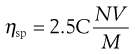
In the case of a capillary tube then the two boundary layers meet at the centre of the tube, such that the velocity distribution is parabolic (Fig. 6.3). With an increase in either the diameter of the tube or the fluid velocity, the proximity of the two boundary layers is reduced and the velocity profile becomes flattened at the centre (Fig. 6.3).

Fig. 6.3 Velocity distributions across a circular cross-section pipe.

Laminar, transitional and turbulent flow

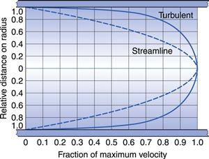
The conditions under which a fluid flows through a pipe, for example, can markedly affect the character of the flow. The type of flow that occurs can be best understood by reference to experiments conducted in 1883 by Reynolds who used an apparatus (Fig. 6.4) which consisted of a horizontal, straight glass tube through which the fluid flowed under the influence of a force provided by a constant head of water. At the centre of the inlet of the tube, a fine stream of dye was introduced. At low flow rates the dye formed a coherent thread which remained undisturbed in the centre of the tube and grew very little in thickness along the length. This type of flow is described as streamlined or laminar flow, and the liquid is considered to flow as a series of concentric cylinders in a manner analogous to an extending telescope.

Fig. 6.4 Reynolds’ apparatus.

If the speed of the fluid is increased, a critical velocity is reached at which the thread begins to waver and then to break up, although no mixing occurs. This is known as transitional flow. When the velocity is increased to higher values the dye instantaneously mixes with the fluid in the tube, as all order is lost and irregular motions are imposed on the overall movement of the fluid: such flow is described as turbulent flow. In this type of flow, the movement of molecules is totally haphazard, although the average movement will be in the direction of flow.

Reynolds’ experiments indicated that the flow conditions were affected by four factors, namely, the diameter of the pipe and the viscosity, density and velocity of the fluid. Furthermore, it was shown that these factors could be combined to give the following equation:

(6.14)

where ρ is the density, u is the velocity, η is the dynamic viscosity of the fluid and d is the diameter of the circular cross-section of the pipe. Re is known as Reynolds’ number and, provided compatible units are used, it will be dimensionless.

Values of Reynolds’ number in a circular cross-section pipe have been determined that can be associated with a particular type of flow. If it is below 2000, then streamlined (i.e. to streamlined) flow will occur, but if it is above 4000, then flow will be turbulent. In between these two values the nature of the flow will depend upon the surface over which the fluid is flowing. For example, if the surface is smooth then streamlined flow may not be disturbed and may exist at values of Reynolds’ number above 2000. However, if the surface is rough or the channel tortuous then flow may well be turbulent at values below 4000, and even as low as 2000. Consequently, although it is tempting to state that values of Reynolds’ number between 2000 and 4000 are indicative of transitional flow, such a statement would only be correct for a specific set of conditions. This also explains why it is difficult to demonstrate transitional flow practically.

Nevertheless, Reynolds’ number is still an important parameter and can be used to predict the type of flow that will occur in a particular situation. The reason why it is important to know the type of flow which is occurring is that whereas with streamlined flow there is no component at right angles to the direction of flow, so that fluid cannot move across the tube, this component is strong for turbulent flow and interchange across the tube is rapid. Thus in the latter case, for example, mass will be rapidly transported, whereas in streamlined flow the fluid layers will act as a barrier to such transfer which can only occur by molecular diffusion.

Determination of the flow properties of simple fluids

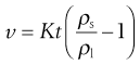
A wide range of instruments exists that can be used to determine the flow properties of Newtonian fluids. However, only some of these are capable of providing data that can be used to calculate viscosities in fundamental units. The design of many instruments precludes the calculation of absolute viscosities as they are capable of providing data only in terms of empirical units.

Not all the available types of instrument used to measure viscosity will be described in this Chapter but it will be limited to simple instruments specified in various official pharmacopoeias.

Capillary viscometers

A capillary viscometer can be used to determine viscosity provided that the fluid is Newtonian and the flow is streamlined. The rate of flow of the fluid through the capillary is measured under the influence of gravity or an externally applied pressure.

Ostwald U-tube viscometer.

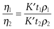
Such instruments are described in pharmacopoeias and are the subject of a specification of the International Organization for Standardization (ISO). A range of capillary bores is available and an appropriate one should be selected so that a flow time for the fluid of approximately 200 seconds is obtained; the wider-bore viscometers are thus for use with fluids of higher viscosity. For fluids where there is a viscosity specification in a pharmacopeia, the size of instrument that must be used in the determination of their viscosity is stated.

The viscometer is shown in Figure 6.5 and liquid is introduced through arm V up to mark G using a pipette long enough to prevent wetting the sides of the tube. The viscometer is then clamped vertically in a constant-temperature water bath and allowed to reach the required temperature. The level of the liquid is adjusted and is then blown or sucked into tube W until the meniscus is just above mark E. The time for the meniscus to fall between marks E and F is then recorded. Determinations should be repeated until three readings all within 0.5 seconds are obtained. Care should be taken not to introduce air bubbles and that the capillary does not become partially occluded with small particles.

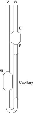
Fig. 6.5 A U-tube viscometer.

The maximum shear rate, γ_m, is given by:

(6.15)

where ρ is the density of the fluid, g the acceleration due to gravity, r_c the radius of the capillary and η the absolute viscosity. Consequently, for a fluid of viscosity 1 mPa s, the maximum shear rate is approximately 2 × 10³ s⁻¹ if the capillary has a diameter of 0.64 mm, but it will be of the order of 10² s⁻¹ for a fluid with a viscosity of 1490 mPa s if the capillary has a diameter of 2.74 mm.

Suspended-level viscometer.

This instrument is a modification of the U-tube viscometer which avoids the need to fill the instrument with a precise volume of fluid. It also addresses the fact that the pressure head in the U-tube viscometer is continually changing as the two menisci approach one another. This instrument is also described in pharmacopoeias and is shown in Figure 6.6.

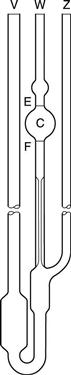
Fig. 6.6 A suspended-level viscometer.

A volume of liquid which will at least fill bulb C is introduced via tube V. The only upper limit on the volume used is that it should not be so large as to block the ventilating tube Z. The viscometer is clamped vertically in a constant-temperature water bath and allowed to attain the required temperature. Tube Z is closed and fluid is drawn into bulb C by the application of suction through tube W until the meniscus is just above the mark E. Tube W is then closed and tube Z opened so that liquid can drain away from the bottom of the capillary. Tube W is then opened and the time the fluid takes to fall between marks E and F is recorded. If at any time during the determination the end of the ventilating tube Z becomes blocked by the liquid, the experiment must be repeated. The same criteria for reproducibility of timings described with the U-tube viscometer must be applied.

Because the volume of fluid introduced into the instrument can vary between the limits described above, this means that measurements can be made at a range of temperatures without the need to adjust the volume.

Calculation of viscosity from capillary viscometers

Poiseuille’s Law states that for a liquid flowing through a capillary tube:

(6.16)

where r is the radius of the capillary, t is the time of flow, P is the pressure difference across the ends of the tube, L is the length of the capillary and V is the volume of liquid. As the radius and length of the capillary as well as the volume flowing are constants for a given viscometer, then:

(6.17)

where K is equal to .

The pressure difference, P, depends upon the density, ρ, of the liquid, the acceleration due to gravity, g, and the difference in heights of the two menisci in the two arms of the viscometer. Because the value of g and the level of the liquids are constant, these can be included in a constant and Equation 6.17 can be written for the viscosities of an unknown and a standard liquid:

(6.18)

(6.19)

Thus, when the flow times for two liquids are compared using the same viscometer, division of Equation 6.18 by Equation 6.19 gives:

(6.20)

and reference to Equation 6.4 shows that Equation 6.20 will yield the viscosity ratio.

However, as Equation 6.3 indicates that the kinematic viscosity is equal to the dynamic viscosity divided by the density, then Equation 6.20 may be rewritten as:

(6.21)

For a given viscometer a standard fluid such as water can be used for the purposes of calibration. Then, Equation 6.21 may be rewritten as:

(6.22)

where c is the viscometer constant.

This equation justifies the continued use of the kinematic viscosity as it means that liquids of known viscosity but of differing density from the test fluid can be used as the standard. A series of oils of given viscosity are available commercially and are recommended for the calibration of viscometers if water cannot be used.

Falling-sphere viscometer

This viscometer is based upon Stokes’ Law (see Chapter 5). When a body falls through a viscous medium, it experiences a resistance or viscous drag which opposes the downward motion. Consequently, if a body falls through a liquid under the influence of gravity, an initial acceleration period is followed by motion at a uniform terminal velocity when the gravitational force is balanced by the viscous drag. Equation 6.23 will then apply to this terminal velocity when a sphere of density ρ_s and diameter d falls through a liquid of viscosity η and density ρ₁. The terminal velocity is u and g is the acceleration due to gravity:

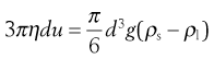(6.23)

The viscous drag is given by the left-hand side of the equation, whereas the right-hand side represents the force responsible for the downward motion of the sphere under the influence of gravity. Equation 6.23 may be used to calculate viscosity by rearrangement to give:

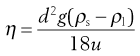(6.24)

Equation 6.3 gives the relationship between η and the kinematic viscosity, such that Equation 6.24 may be rewritten as:

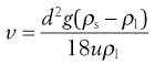(6.25)

In the derivation of these equations it is assumed that the sphere falls through a fluid of infinite dimensions. However, for practical purposes the fluid must be contained in a vessel of finite dimensions and it is therefore necessary to include a correction factor to account for the end and wall effects. The correction normally used is due to Faxen and may be given as:

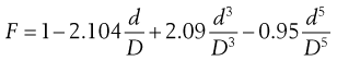(6.26)

where D is the diameter of the measuring tube and d is the diameter of the sphere. The last term in Equation 6.26 accounts for the end effect and may be ignored as long as only the middle third of the depth is used for measuring the velocity of the sphere. In fact, the middle half of the tube can be used if D is at least 10 times d, and the second and third terms, which account for the wall effects, can be replaced by 2.1 d/D.

The apparatus used to determine u is shown in Figure 6.7. The liquid is placed in the fall tube which is clamped vertically in a constant-temperature bath. Sufficient time must be allowed for temperature equilibration to occur and for any air bubbles to rise to the surface. A steel sphere which has been cleaned and brought to the temperature of the experiment is introduced into the fall tube through a narrow guide tube, the end of which must be below the surface of the fluid under test. The passage of the sphere is monitored by a method that avoids parallax, and the time it takes to fall between the etched marks A and B is recorded. It is usual to take the average of three readings, all of which must be within 0.5%, as the fall time, t, to calculate the viscosity. If the same sphere and fall tube are used then Equation 6.25 reduces to:

(6.27)

where K is a constant that may be determined by the use of a liquid of known kinematic viscosity.

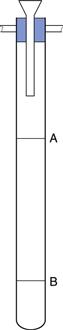
Fig. 6.7 A falling-sphere viscometer.

A number of pharmacopoeias specify the use of a viscometer of this type; it is sometimes referred to as a falling-ball viscometer. Like capillary viscometers, it should only be used with Newtonian fluids.

Non-Newtonian fluids

The characteristics described in the previous sections apply only to fluids that obey Newton’s Law (Eqn 6.1) and which are consequently referred to as Newtonian. However, most pharmaceutical fluids do not obey this law as the viscosity of many fluids varies with the rate of shear. The reason for these deviations is that they are not simple fluids such as water and syrup, but may be disperse or colloidal systems, including emulsions, suspensions and gels. These materials are known as non-Newtonian and with the increasing use of sophisticated polymer-based delivery systems, more examples of such behaviour are found in pharmaceutical science.

Types of non-Newtonian behaviour

More than one type of deviation from Newton’s law can be recognized, and the type of deviation that occurs can be used to classify the particular material.

If a Newtonian fluid is subjected to an increasing rate of shear, γ, and the corresponding shear stress, σ, recorded then a plot of γ against σ will produce the linear relationship shown in Figure 6.8a. Such a plot is usually referred to as a flow curve or rheogram. The slope of this plot will give the viscosity of the fluid and its reciprocal the fluidity. Equation 6.1 indicates that this line will pass through the origin.

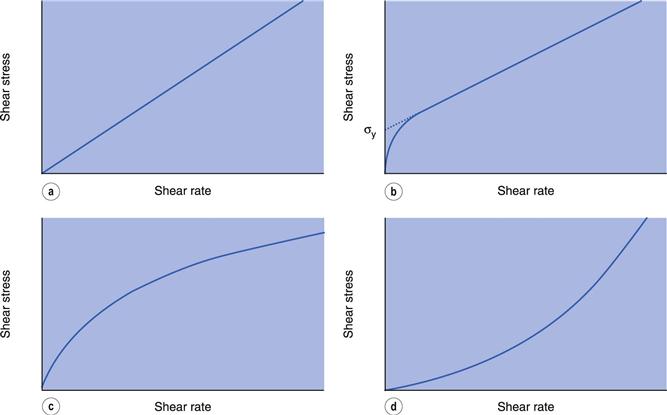
Fig. 6.8 Flow curves or rheograms representing the behaviour of various materials. (a) Newtonian, (b) plastic, (c) pseudoplastic and (d) dilatant.

Plastic (or Bingham) flow

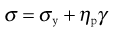
Figure 6.8b indicates an example of plastic flow or Bingham flow, when the rheogram does not pass through the origin but intersects with the shear stress axis at a point usually referred to as the yield value, σ_y. This implies that a plastic material does not flow until such a value of shear stress has been exceeded, and at lower stresses the substance behaves as a solid (elastic) material. Plastic materials are often referred to as Bingham bodies in honour of the worker who carried out many of the original studies on them. The equation he derived may be given as:

(6.28)

where η_p is the plastic viscosity and σ_y the Bingham yield stress or Bingham value (Fig. 6.8b). The equation implies that the rheogram is a straight line intersecting the shear stress axis at the yield value σ_y. In practice, flow will begin to occur at a lower shear stress than σ_y and the flow curve gradually approaches the extrapolation of the linear portion of the line shown in Figure 6.8b. This extrapolation will also give the Bingham or apparent yield value; the slope is the plastic viscosity.

Plastic flow is exhibited by concentrated suspensions, particularly if the continuous phase is of high viscosity or if the particles are flocculated.

Pseudoplastic flow

The rheogram shown in Figure 6.8c arises at the origin and, as no yield value exists, the material will flow as soon as a shear stress is applied; the slope of the curve gradually decreases with increasing rate of shear. The viscosity is derived from the slope and therefore decreases as the shear rate is increased. Materials exhibiting this behaviour are said to be pseudoplastic, and no single value of viscosity can be considered as characteristic. The viscosity, which can only be calculated from the slope of a tangent drawn to the curve at a specific point, is known as the apparent viscosity. It is only of any use if quoted in conjunction with the shear rate at which the determination was made. However, it would need several apparent viscosities to be determined in order to characterize a pseudoplastic material so perhaps the most satisfactory representation is by means of the entire flow curve. However, it is frequently noted that at higher shear stresses the flow curve tends towards linearity, indicating that a minimum viscosity has been attained. When this is the case, such a viscosity can be a useful means of classification.

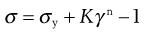
There is no completely satisfactory quantitative explanation of pseudoplastic flow; probably the most widely used is the Power Law, which is given as:

(6.29)

where η′ is a viscosity coefficient and the exponent, n, an index of pseudoplasticity. When n = 1, then η′ becomes the dynamic viscosity (η) and Equation 6.29 the same as Equation 6.1, but as a material becomes more pseudoplastic then the value of n will fall. In order to obtain the values of the constants in Equation 6.29, log σ must be plotted against log γ, from which the slope will produce n and the intercept η′. The Equation may only apply over a limited range (approximately one decade) of shear rates, and so it may not be applicable for all pharmaceutical materials and other models may have to be considered in order to fit the data. For example, the model known as Herschel–Bulkley can be given as:

(6.30)

where K is a viscosity coefficient. This can be of use for flow curves that are curvilinear and which intersect with the stress axis.

The materials that exhibit this type of flow include aqueous dispersions of natural and chemically modified hydrocolloids, such as tragacanth, methylcellulose and carmellose, and synthetic polymers such as polyvinylpyrrolidone and polyacrylic acid. The presence of long, high molecular weight molecules in solution results in their entanglement with the association of immobilized solvent. Under the influence of shear, the molecules tend to become disentangled and align themselves in the direction of flow. They thus offer less resistance to flow and this, together with the release of some of the entrapped water, accounts for the lower viscosity. At any particular shear rate, equilibrium will be established between the shearing force and the molecular re-entanglement brought about by Brownian motion.

Dilatant flow

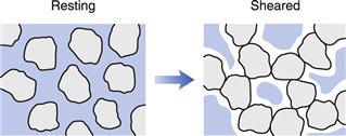
The opposite type of flow to pseudoplasticity is depicted by the curve in Figure 6.8d, in that the viscosity increases with increase in shear rate. As such materials increase in volume during shearing, they are referred to as dilatant and exhibit shear thickening. An equation similar to that for pseudoplastic flow (Eqn 6.29) may be used to describe dilatant behaviour, but the value of the exponent n will be greater than 1 and will increase as dilatancy increases.

This type of behaviour is less common than plastic or pseudoplastic flow, but may be exhibited by dispersions containing a high concentration (≈ 50%) of small, deflocculated particles. Under conditions of zero shear, the particles are closely packed and the interparticulate voids are at a minimum (Fig. 6.9), which the vehicle is sufficient to fill and at low shear rates such as those created during pouring this is still the case. As the shear rate is increased the particles become displaced from their uniform distribution and the clumps that are produced result in the creation of larger voids, into which the vehicle drains, so that the resistance to flow is increased and viscosity rises. The effect is progressive with increase in shear rate until eventually the material may appear paste-like as flow ceases. Fortunately, the behaviour is reversible and removal of the shear stress results in the re-establishment of the fluid nature.

Fig. 6.9 Representation of the cause of dilatant behaviour.

Dilatancy can be a problem during the processing of dispersions and the granulation of tablet masses when high-speed mills and blenders are employed. If the material being processed becomes dilatant in nature then the resultant solidification could overload and damage the motor. Changing the batch or supplier of the ingredient used could lead to processing problems that can only be avoided by rheological evaluation of the dispersions prior to their introduction in the production process.

Time-dependent behaviour

In the description of the different types of non-Newtonian behaviour it was implied that although the viscosity of a fluid might vary with shear rate, it was independent of the length of time that the shear rate was applied, and also that replicate determinations at the same shear rate would always produce the same viscosity. This must be considered as the ideal situation, as most non-Newtonian materials are colloidal in nature and the flowing elements, whether they are particles or macromolecules, may not adapt immediately to the new shearing conditions.

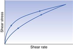
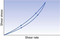
Therefore, when such a material is subjected to a particular shear rate, the shear stress and consequently the viscosity will decrease with time. Furthermore, once the shear stress has been removed, even if the breakdown in structure is reversible, it may not return to its original condition (rheological ground state) instantly. The common feature of all these materials is that if they are subjected to a gradually increasing shear rate, which in turn is decreased to zero, the down curve of the rheogram will be displaced with regard to the up curve and a hysteresis loop will be included (Fig. 6.10). In the case of plastic and pseudoplastic materials, the down curve will be displaced to the right of the up curve (Fig. 6.10), whereas for dilatant substances the reverse will be true (Fig. 6.11). The presence of the hysteresis loop indicates that a breakdown in structure has occurred, and the area within the loop may be used as an index of the degree of breakdown.

Fig. 6.10 Rheogram produced by a thixotropic pseudoplastic material.

Fig. 6.11 Rheogram produced by a thixotropic dilatant material.

The term that is used to describe such behaviour is thixotropy, which means ‘to change by touch’. Although the term should only strictly be applied to an isothermal sol-gel transformation, it has become common to describe any material that exhibits a reversible time-dependent decrease in apparent viscosity as thixotropic. Such systems are usually composed of asymmetric particles or macromolecules that are capable of interacting by numerous secondary bonds to produce a loose three-dimensional structure, so that the material is gel-like when unsheared. The energy imparted during shearing disrupts these bonds, so that the flowing elements become aligned and the viscosity falls, as a gel-sol transformation has occurred. When the shear stress is eventually removed, the structure will tend to reform, although the process is not immediate but will increase with time as the molecules return to the original state under the influence of Brownian motion. Furthermore, the time taken for recovery, which can vary from minutes to days depending upon the system, will be directly related to the length of time the material was subjected to the shear stress, as this will affect the degree of breakdown.

In some cases the structure that has been destroyed is never recovered, no matter how long the system is left unsheared. Repeat determinations of the flow curve will then produce only the down curve which was obtained in the experiment that resulted in the destruction. It is suggested that such behaviour be referred to as ‘shear destruction’ rather than thixotropy which, as will be appreciated from the above, is a misnomer in this case.

An example of such behaviour is the gels produced by high molecular weight polysaccharides, which are stabilized by large numbers of secondary bonds. Such systems undergo extensive reorganization during shearing such that the three-dimensional structure is reduced to a two-dimensional one; the gel-like nature of the original is then never recovered.

The occurrence of such complex behaviour creates problems in the quantification of the viscosity of these materials because not only will the apparent viscosity change with shear rate, but there will also be two viscosities that can be calculated for any given shear rate (i.e. from the up curve and the down curve). It is usual to attempt to calculate one viscosity for the up curve and another for the down curve but this requires each of the curves to achieve linearity over some of its length, otherwise a defined shear rate must be used; only the former situation is truly satisfactory. Each of the lines used to derive the viscosity may be extrapolated to the shear stress axis to give an associated yield value. However, only the one derived from the up curve has any significance, as that derived from the down curve will relate to the broken-down system.

Consequently, the most useful index of thixotropy can be obtained by integration of the area contained within the loop. This will not, of course, take into account the shape of the up and down curves, and so two materials may produce loops of similar area but with completely different shapes, representing totally different types of flow behaviour. In order to prevent confusion, it is best to adopt a method whereby an estimate of area is accompanied by yield value(s). This is particularly important when complex up curves exhibiting bulges are obtained, although it is now acknowledged that when these have been reported in the literature, they might well have been a consequence of the design of the instrument, rather than providing information on the three-dimensional structure of the material. The evidence for this is based on the flow curves produced using more modern instruments, which do not exhibit the same, if any, bulges.

Determination of the flow properties of non-Newtonian fluids

With such a wide variety of rheological behaviour, it is extremely important to carry out measurements that will produce meaningful results. It is crucial therefore not to use a determination of viscosity at one shear rate which, although perfectly acceptable for a Newtonian fluid, would produce results which are useless for any comparative purposes. Figure 6.12 shows rheograms that represent the four different types of flow behaviour, all of which intersect at point A, which is equivalent to a shear rate of 100 s⁻¹. Therefore, if a measurement was made at this one shear rate, all four materials would be shown to have the same viscosity (σ/γ = 0.01 Pa s) although they each exhibit different characteristics. Single-point determinations are probably an extreme example but are used here to emphasize the importance of properly designed experiments.

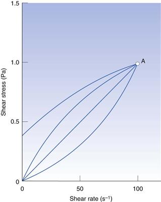
Fig. 6.12 Explanation of the effect of single-point viscosity determination and the resultant errors.

Rotational viscometers

These instruments rely on the viscous drag exerted on a body when it is rotated in the fluid to determine its viscosity. They should really be referred to as rheometers since nowadays they are suitable for use with both Newtonian and non-Newtonian materials. Their major advantage is that wide ranges of shear rate can be achieved and if a programme of shear rates can be selected automatically, then a flow curve or rheogram for a material may be obtained directly. A number of commercial instruments are available which vary from those that can be used as simple on-line devices to sophisticated multi-function machines. However, all share a common feature in that various measuring geometries can be used; often these have been concentric cylinder (or couette) and cone-plate, although parallel-plate is becoming more widely used.

Concentric cylinder.

In this geometry there are two coaxial cylinders of different diameters, the outer forming the cup containing the fluid in which the inner cylinder or bob is positioned centrally (Fig. 6.13). In older types of instrument the outer cylinder is rotated and the viscous drag exerted by the fluid is transmitted to the inner cylinder as a torque inducing its rotation which can be measured by a transducer or a fine torsion wire. The stress on this inner cylinder (when, for example, it is suspended on a torsion wire) is indicated by the angular deflection, θ, once equilibrium (i.e. steady flow) has been attained. The torque, T, can then be calculated from:

(6.31)

where C is the torsional constant of the wire. The viscosity is then given by:

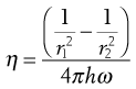(6.32)

where r₁ and r₂ are the radii of the inner and outer cylinders respectively, h is the height of the inner cylinder, and ω is the angular velocity of the outer cylinder.

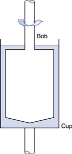
Fig. 6.13 Concentric cylinder geometry.

Cone-plate.

The cone-plate geometry comprises a flat circular plate with a wide-angle cone placed centrally above it (Fig. 6.14). The tip of the cone just touches the plate and the sample is loaded into the included gap. When the plate is rotated the cone will be caused to rotate against a torsion wire in the same way as the inner cylinder described above. Provided the gap angle is small (less than 1°), the viscosity will be given by:

(6.33)

where ω is the angular velocity of the plate, T is the torque, r is the radius of the cone and α is the angle between the cone and the plate.

Fig. 6.14 Cone-plate geometry.

Parallel plate.

This only differs from cone-plate in that the cone is replaced by a flat plate which is similar to the opposing part of the geometry (Fig. 6.15). The viscosity is given by:

(6.34)

where in this case r is the diameter of the plates and h the gap between them.

Fig. 6.15 Parallel plate geometry.

Rheometers

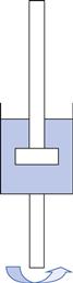
From Equation 6.2 it can be seen that the viscosity of a fluid can be calculated by dividing the shear stress by the shear rate. However, in order to do this it is essential to have an instrument that is capable of imposing either a constant shear rate and measuring the resultant shear stress or a constant shear stress when measurement of the induced shear rate is required. The first type of instrument is referred to as controlled-rate (or strain) whereas the latter is known as controlled-stress. As is the case with most scientific measurements, the history of the development of the instrumentation can be instructive in understanding the way in which they work. The MacMichael controlled-rate (or controlled-strain) viscometer, which was patented in 1918, had a cup which contained the fluid under test and could be rotated at just one speed. A 5 mm thick disk suspended on a torsion wire was immersed in the fluid in the cup (Fig. 6.16). The viscous drag exerted by the fluid caused the disk to rotate, which in turn produced a deflection in the torsion wire to an equilibrium position which was inversely related to the viscosity. An early modification was to couple a gearbox to the synchronous electric motor so that a series of speeds (rates of shear) could be employed. The change from a synchronous, first, to a direct current motor and then a step (or stepper) motor has obviated the need to include a gearbox although these are still incorporated in some instruments as a means of extending the range of shear rates that can be applied.

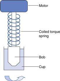
Fig. 6.16 A diagrammatic representation of a controlled-rate rheometer.

The absolute viscosity could not be determined with these early instruments, but the use of a calibrated torsion wire and a defined measuring geometry (such as concentric cylinder or cone-plate) made this possible. Perhaps the most significant improvements which have been made to the technology are the replacement of the torsion wire with more sophisticated torque measurement devices, sometimes referred to as dynamometers. Their introduction meant that the cup in Figure 6.16 could be fixed and only the upper part of the geometry needed to be driven by the motor via a coiled spring (Fig. 6.17): the degree of flexure of the spring is, like the torsion wire that it replaced, inversely related to the resistance to flow (i.e. viscosity) of the fluid. Although this modification enabled the viscosity to be read directly off a scale and instruments to be automated, the spring had to have a low elastic modulus and the weight of the measuring geometry which it supported created inertia which had to be overcome once the motor was started. This resulted in a lag period before the bob began to rotate, followed by a rapid acceleration which, in turn, produced an overshoot. This type of behaviour was very apparent with the Ferranti-Shirley viscometer which was widely used with pharmaceutical semi-solids in the 1960s and 1970s. The instrument was highly automated for its time and produced a plot of a flow curve in real time on an X-Y recorder. However, the inertial overshoot was apparent as bulges in the flow curves that were obtained but, unfortunately, these artefacts were taken by some workers to represent rheological characteristics of the material. Advances in electronics meant that the spring could be replaced by a stiffer torsion strip or bar which is only deflected by a few degrees. The concomitant improvements in micro-processors enabled instrumental control and data collection to be integrated so that not only did measurements become automatic but also data processing was virtually instantaneous.

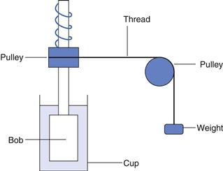
Fig 6.17 A diagrammatic representation of a controlled rate rheometer with a coiled spring torque measuring device.

The first controlled-stress viscometer was described by Stormer in 1909 and was based on a cup and bob geometry where the outer cup was stationary and the inner one was immersed in the liquid under test. The inner cylinder was rotated at a constant stress produced by a weight attached to a length of thread which was wrapped around a horizontal pulley on the shaft of the cylinder and then passed over a vertical pulley so that it fell under the influence of gravity (Fig. 6.18). The rate of rotation was measured with the aid of a stopwatch and an eagle-eyed operator. The most common way of using the instrument was to determine the weight that produced a predetermined rate of rotation: although this was useful for comparative purposes, it did not allow the calculation of absolute viscosities. Almost 60 years elapsed before workers attempted to adapt this instrument to operate at very low stresses and measure displacement over long times. Such experiments were known as creep tests and once the technology became available a similar enhancement in their application occurred as it did with controlled-rate instruments. In this instance, the most significant improvements were the use of air bearings to provide both lateral and axial support, the use of optical encoders to measure radial displacement and the addition of drag-cup motors to produce the torque. The latter not only allowed the smooth control of torque but also had very low inertia so that low stresses could be applied.

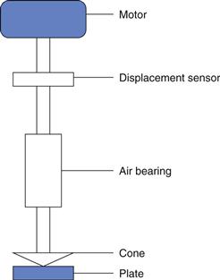
Fig. 6.18 A diagrammatic representation of a controlled-stress rheometer.

The design of instruments with the capacity to operate as controlled-strain or controlled-stress has now advanced such that both types of test can be conducted with the same instrument. A generalised representation of the instruments is shown in Figure 6.19. The bearing supports the changeable measuring geometry and may be enclosed in a unit which also houses the motor and the displacement sensor. When used in the controlled-stress mode, the current to the motor generates a torque which rotates the measuring geometry against the resistance of the sample. The resultant displacement is measured by the sensor so that the speed can be calculated. The difference when operated in controlled-strain mode is that there is feedback to the motor from the sensor so that instead of providing a predetermined stress, the torque necessary to maintain a given strain is measured. In both cases, since the rate of shear and shear rate are available the viscosity can be calculated. Also both instrumental designs can be used for dynamic testing using forced oscillation, and thus characterize viscoelastic properties. As in many aspects of modern life, the developments in computing hardware and software have contributed significantly to advances in the design and use of rheometers.

Fig.6.19 A schematic diagram of a rheometer that can operate in a variety of modes.

Viscoelasticity

In the experiments described for rotational viscometers, two observations are often made with pharmaceutical materials:

1. With cone-plate geometry, the sample appears to ‘roll up’ at high shear rates and is ejected from the gap.

2. With concentric cylinder geometry, the sample will climb up the spindle of the rotating inner cylinder (Weissenberg effect).

The cause of both these phenomena is the same; that is, the liquids are not exhibiting purely viscous behaviour but are viscoelastic. Such materials display solid and liquid properties simultaneously, and the factor that governs the actual behaviour is time. A whole spectrum of viscoelastic behaviour exists, for materials that are predominantly either liquid or solid. Under a constant stress, all these materials will dissipate some of the energy in viscous flow and store the remainder, which will be recovered when the stress is removed. The type of response can be seen in Figure 6.20a, where a small, constant stress has been applied to a 2% gelatin gel and the resultant change in shape (strain) is measured.

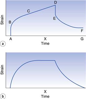
Fig. 6.20 Creep (or compliance) curves for (a) an uncrosslinked system and (b) a crosslinked system.

In the region A–B an initial elastic jump is observed, followed by a curved region B–C when the material is attempting to flow as a viscous fluid but is being retarded by its solid characteristics. At longer times, equilibrium is established, so that for a system like this, which is ostensibly liquid, viscous flow will eventually predominate and the curve will become linear (C–D). If the concentration of gelatin in the gel had been increased to 30% then the resultant material would be more solid-like and no flow would be observed at longer times so that the curve would level out as shown in Figure 6.20b. In the case of the liquid system, when the stress is removed only the stored energy will be recovered, and this is represented by an initial elastic recoil (D–E, Fig. 6.20a) equivalent to the region A–B and a retarded response E–F equivalent to B–C. There will be a displacement from the starting position (F–G) and this will be related to the amount of energy lost during viscous flow. For the higher-concentration gel, all the energy will be recovered, so that only the regions D–E and E–F are observed.

This significance of time can be observed from the point X on the time axis. Although both systems are viscoelastic, and, indeed, are produced by different concentrations of the same biopolymer, in Figure 6.20a the sample is flowing like a high-viscosity fluid, whereas in Figure 6.20b it is behaving like a solid.

Creep testing

Both the experimental curves shown in Figure 6.20 are examples of a phenomenon known as creep. If the measured strain is divided by the stress – which, it should be remembered, is constant – then a compliance will be derived. As compliance is the reciprocal of elasticity, it will have the units m² N⁻¹ or Pa⁻¹. The resultant curve, which will have the same shape as the original strain curve, then becomes known as a creep compliance curve. If the applied stress is below a certain limit (known as the linear viscoelastic limit), it will be directly related to the strain and the creep compliance curve will have the same shape and magnitude regardless of the stress used to obtain it. This curve therefore represents a fundamental property of the material, and derived parameters are characteristic and independent of the experimental method. For example, although it is common to use either cone-plate or concentric cylinders with viscoelastic pharmaceuticals, almost any measuring geometry can be used provided the shape of the sample can be defined and maintained throughout the experiment.

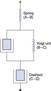
It is common to analyse the creep compliance curve in terms of a mechanical model, an example of which is shown in Figure 6.21. This figure also indicates the regions on the curve shown in Figure 6.20a to which the components of the model relate. Thus, the instantaneous jump can be described by a perfectly elastic spring and the region of viscous flow by a piston fitted into a cylinder containing an ideal Newtonian fluid (this arrangement is referred to as a dashpot). In order to describe the behaviour in the intermediate region, it is necessary to combine both these elements in parallel, such that the movement of the spring is retarded by the fluid in the dashpot; this combination is known as a Voigt unit. It is implied that the elements of the model do not move until the preceding one has become fully extended. Although it is not feasible to associate the elements of the model with the molecular arrangement of the material, it is possible to ascribe a viscosity to the fluids in each cylinder and elasticity (or compliance) to each spring.

Fig. 6.21 Mechanical model representation of a creep compliance curve.

Thus, a viscosity can be calculated for the single dashpot (Fig. 6.21) from the reciprocal of the slope of the linear part of the creep compliance curve. This viscosity will be several orders of magnitude greater than that obtained by the conventional rotational techniques. It may be considered to be that of the rheological ground state (η₀) as the creep test is non-destructive and should produce the same viscosity however many times it is repeated on the same sample. This is in direct contrast to continuous shear measurements, which destroy the structure being measured and with which it is seldom possible to obtain the same result in subsequent experiments on the same sample. The compliance (J₀) of the spring can be measured directly from the height of region A–B (Fig. 6.20a) and the reciprocal of this value will yield the elasticity, E₀. It is often the case that this value, together with η₀, provides an adequate characterization of the material.

However, the remaining portion of the curve can be used to derive the viscosity and elasticity of the elements of the Voigt unit. The ratio of the viscosity to the elasticity is known as the retardation time, τ, and is a measure of the time taken for the unit to deform to 1/e of its total deformation. Consequently, more rigid materials will have longer retardation times and the more complex the material, the greater the number of Voigt units that are necessary to describe the creep curve.

It is also possible to use a mathematical expression to describe the creep compliance curve:

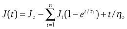(6.35)

where J(t) is the compliance at time t, and J_i and τ_i are the compliance and retardation time, respectively, of the ‘ith’ Voigt unit. Both the model and the mathematical approach interpret the curve in terms of a line spectrum. It is also possible to produce a continuous spectrum in terms of the distribution of retardation times.

What is essentially the reverse of the creep compliance test is the stress relaxation test, where the sample is subjected to a predetermined strain and the stress required to maintain that strain is measured as a function of time. In this instance, a spring and dashpot in series (known as a Maxwell unit) can be used to describe the behaviour. Initially the spring will extend instantaneously, and will then contract more slowly as the piston flows in the dashpot. Eventually the spring will be completely relaxed but the dashpot will be displaced, and in this case the ratio of viscosity to elasticity is referred to as the relaxation time.

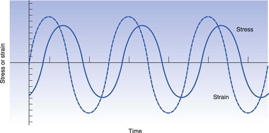
Dynamic testing

Both creep and relaxation experiments are considered to be static tests. Viscoelastic materials can also be evaluated by means of dynamic experiments, whereby the sample is exposed to a forced sinusoidal oscillation and the transmitted stress measured. Once again, if the linear viscoelastic limit is not exceeded then the stress will also vary sinusoidally (Fig. 6.22). However, because of the nature of the material, energy will be lost so that the amplitude of the stress wave will be less than that of the strain wave behind which it will also lag. If the amplitude ratio and the phase lag can be measured, then the elasticity, referred to as the storage modulus, G′, is given by:

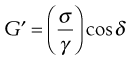(6.36)

where σ is the stress, γ is the strain and δ is the phase lag. A further modulus, G″, known as the loss modulus, is given by:

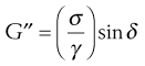(6.37)

This can be related to viscosity, η′, by:

(6.38)

where ω is the frequency of oscillation in rad (s⁻¹). From Equations 6.36 and 6.37 it can be seen that:

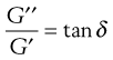(6.39)

and tan δ is known as the loss tangent. Thus, a perfectly elastic material would produce a phase lag of 0°, whereas for a perfect fluid it would be 90°.

Fig. 6.22 Sine waves showing the stress wave lagging behind the strain wave during dynamic testing.

Finally, the concepts of liquid-like and solid-like behaviour can be explained by the dimensionless Deborah number (De), which finds expression as:

(6.40)

where τ is a characteristic time of the material and T is a characteristic time of the deformation process. For a perfectly elastic material (solid), τ will be infinite, whereas for a Newtonian fluid it will be zero. With any material, high Deborah numbers can be produced either by high values of τ or by small values of T. The latter will occur in situations where high rates of strain are experienced, for example slapping water with the hand. Also, even solid materials would flow if a high enough stress was applied for a sufficiently long time.

The application of rheology in pharmaceutical formulation

The components used to make a formulation may not only affect the physical and release characteristics of the product but may also guide it to the site of absorption. In some cases it may be possible to exploit the properties of the excipients such that the dosage form is retained at a specific location in the body. This approach is often necessary for locally acting products which are used to treat or prevent diseases of, for example, the eye and the skin. To treat conditions in the eye an aqueous solution of the drug is delivered to the precorneal area by means of a dropper. If the solution is Newtonian and of low viscosity, then it will be rapidly cleared form the eye as a result of reflex tear production and blinking. The resultant short residence time means that an effective concentration will only be attained for brief periods following dosing so that treatment is pulsatile. However, if a water-soluble polymer is added to the formulation, such that the viscosity is within the range of 15–30 mPa s, then the residence time increases as does the bioavailability. Addition of excipients that make the product pseudoplastic will facilitate blinking and this may improve acceptance and compliance by the patient. If the product can be made viscoelastic then solutions of higher consistency may be tolerated. This can be achieved in the eye if a polymeric solution is designed to be Newtonian when it is instilled, but then undergoes a sol-gel transition in situ in reaction to the change in environment such as temperature, pH or ion content. Polyvinyl alcohol, cellulose ethers and esters and sodium alginate are all examples of polymers which have been used as viscolysers in eye drops. Polyacrylic acid and cellulose acetate phthalate have been claimed to produce reactive systems. The formulation of eye drops and the importance of viscosity in formulation of ocular delivery systems are discussed further in Chapter 41.

The ointments and creams which are applied to the skin to deliver a drug which has a local action, such as a corticosteroid or anti-infective agent, are usually semi-solids. Their rheological properties need to be assessed after manufacture and during the shelf-life in order to ensure that the product is physically stable; this is important because the rate of release of the drug and the concentration at the site of action is related to the apparent viscosity. Since these products are packaged in flexible tubes then rheological measurements will also indicate whether the product can be readily removed from the container (see also Chapter 39).

Knowledge of the flow properties of a product such as a gel for topical application can be used to predict patient acceptability, since humans can detect small changes in viscosity during activities such as rubbing an ointment on the skin, shaking ketchup from a bottle or squeezing toothpaste from a tube. Since the ability of the body to act as a rheometer involves the unconscious coordination of a number of senses, the term psychorheology has been adopted by workers in this field. All three situations provide examples of the advantages of designing a formulation which has a yield stress and exhibits plastic or pseudoplastic behaviour so that the patient only has to apply the appropriate shear rate.

Transdermal delivery systems (often referred to as patches) are used to deliver drug across the skin at a rate which means that they can be left on the skin for periods of up to a week. The drug can either be incorporated in a reservoir or dissolved in the layer of adhesive which holds the device on the skin (Chapter 39). The rheological properties of the adhesive can therefore be used to predict and control not only the adhesion but also the rate of absorption of the drug. The latter can be used to estimate the length of time that device needs to be applied to the skin.

When a dosage form is intended to be administered perorally, so that the active ingredient can be absorbed from the gastrointestinal tract, then the gastrointestinal transit time plays a major role in the extent and amount of drug which appears in the blood stream. The first phase of gastrointestinal transit is gastric emptying, which is in part dictated by the rise in viscosity of stomach contents in the presence of food. The consequential increase in gastric residence time and fall in the dissolution rate of the active ingredient can lead to a reduction in the rate, but not necessarily the extent, of absorption. Such effects can be exploited by the pharmaceutical formulator, for example, by including a gel-forming polymer in the formulation, since this can simulate in vivo the effect exerted by food. However, its use as a means of prolonging the duration of action of an orally administered medicine needs to be thoroughly understood particularly in relation to the effect of the presence and nature of food, since any benefit could be lost by, for example, administration of the dosage form following a high-fat meal. Many solid sustained-release dosage forms depend upon the inclusion of high molecular weight polymers for their mode of action, and the viscosity of a particular polymer both in dilute solution and as a swollen gel is used to aid the selection of the most suitable candidate.

A final example of the application of rheology in the design and use of dosage forms is the administration of medicines by intramuscular injection. These are formulated as either aqueous or lipophilic (oily) solutions or suspensions. Following injection, the active ingredient is absorbed more quickly from an aqueous formulation than its lipophilic counterpart. The incorporation of the active ingredient as a suspension in either type of base offers a further opportunity of slowing the rate of release. The influence that the nature of the solvent has on the rate of drug release is in part due to its compatibility with the tissue but its viscosity is also of importance. Although it may be possible to extend the dosing interval by further increasing the viscosity of the oil, it has to be borne in mind that the product needs to be able to be drawn into a syringe via a needle, the diameter of which must not be so large as to alarm or discomfort the patient. Furthermore, adding other excipients such as polymers to the formulation or even just altering the particle size of the suspended particles can induce marked alterations in the rheological properties such that the injection may become plastic, pseudoplastic or dilatant. If it does become plastic, then provided that the yield value is not too high it may be possible to pass through a syringe needle by application of a force which it is reasonable to achieve with a syringe. Quite obviously this will not be the case if the suspension becomes dilatant since as the applied force is increased the product will become more solid. Often the ideal formulation is one which is pseudoplastic because as the force is increased so the apparent viscosity will fall making it easier for the injection to flow through the needle. Ideally the product should also be truly thixotropic since once it has been injected into the muscle then the reduction in shear rate will mean that the bolus will gel and thus form a depot from which release of the drug may be expected to be delayed. The use of appropriate rheological techniques in the development of such products can be beneficial not only to predict their performance in vivo but also to monitor changes in characteristics on storage. This is especially true for suspension formulations, since fine particles have a notorious and, sometimes, malevolent capacity for increasing in size on storage and if because of this a pseudoplastic product becomes dilatant, then it will be impossible to administer it to the patient.

Bibliography

1. Barnes HA, Hutton JF, Walters K. An Introduction to Rheology. Amsterdam: Elsevier Science; 1989.

2. Barnes HA, Schimanski H, Bell D. 30 years of progress in viscometers and rheometers. Applied Rheology. 1999;9:69–76.

3. Barnes HA, Bell D. Controlled-stress rotational rheometry: An historical review. Korea-Australia Rheology Journal. 2003;15:187–196.

4. Lapasin R, Pricl S. Rheology of Industrial Polysaccharides: Theory and Applications. Gaithersburg: Aspen Publishers; 1999.

5. Mezger TG. The Rheology Handbook. Hanover: European Coatings Tech Files; 2011.

Recent Posts

Meta

Categories

Search Engine

Rheology