[level-membership-for-basic-science-category]
Properties of solutions
Michael E. Aulton
Chapter contents
Vapour pressures of solids, liquids and solutions
Hydrogen ion concentration and pH
Dissociation (or ionization) constants; pKa and pKb
Key points
Introduction
The aim of this chapter is to provide information on certain properties of solutions that relate to their applications in pharmaceutical science. This chapter deals mainly with the physicochemical properties of solutions that are important with respect to pharmaceutical systems. These aspects are covered in sufficient detail to introduce the pharmaceutical scientist to these properties to allow an understanding of their importance in dosage form design and drug delivery. Much is published elsewhere in far greater detail and any reader requiring this additional information can trace some of this by referring to the bibliography at the end of the chapter.
Types of solution
Solutions may be classified based on the physical state (i.e. gas, liquid or solid) of the solute(s) and solvent. Although a variety of different types can exist, solutions of pharmaceutical interest virtually all possess liquid solvents. In addition, the solutes are predominantly solid substances. Consequently, most of the information in this chapter is relevant to solutions of solids in liquids.
Vapour pressures of solids, liquids and solutions
An understanding of many of the properties of solutions requires an appreciation of the concept of an ideal solution and its use as a reference system, to which the behaviours of real (non-ideal) solutions can be compared. This concept is itself based on a consideration of vapour pressure. The present section serves as an introduction to the later discussions on ideal and non-ideal solutions.
The kinetic theory of matter indicates that the thermal motion of molecules of a substance in its gaseous state is more than adequate to overcome the attractive forces that exist between the molecules. Thus, the molecules will undergo a completely random movement within the confines of the container. The situation is reversed, however, when the temperature is lowered sufficiently so that a condensed phase is formed. Here the thermal motions of the molecules are now insufficient to overcome completely the intermolecular attractive forces and some degree of order in the relative arrangement of molecules occurs. This condensed state may be either liquid or solid.
If the intermolecular forces are so strong that a high degree of order is brought about, when the structure is hardly influenced by thermal motions, then the substance is usually in the solid state.
In the liquid condensed state, the relative influences of thermal motion and intermolecular attractive forces are intermediate between those in the gaseous and solid states. Thus, the effects of interactions between the permanent and induced dipoles, i.e. the so-called van der Waals forces of attraction, lead to some degree of coherence between the molecules of liquids. Consequently, liquids occupy a definite volume with a surface, unlike gases, and whilst there is evidence of structure within liquids, such structure is much less apparent than in solids.
Although both solids and liquids are condensed systems with cohering molecules, some of the surface molecules in these systems will occasionally acquire sufficient energy to overcome the attractive forces exerted by adjacent molecules. The molecules can therefore escape from the surface to form a vapour phase. If temperature is maintained constant, equilibrium will be established eventually between the vapour phase and the condensed phase. The pressure exerted by the vapour at this equilibrium is referred to as the vapour pressure of the substance.
All condensed systems have the inherent ability to give rise to a vapour pressure. However, the vapour pressures exerted by solids are usually much lower than those exerted by liquids, because the intermolecular forces in solids are stronger than those in liquids. Thus, the escaping tendency for surface molecules is higher in liquids. Consequently, surface loss of vapour from liquids by the process of evaporation is more common than surface loss of vapour from solids by sublimation.
In the case of a liquid solvent containing a dissolved solute, molecules of both solvent and solute may show a tendency to escape from the surface and so contribute to the vapour pressure. The relative tendencies to escape will depend on the relative numbers of the different molecules in the surface of the solution, and on the relative strengths of the attractive forces between adjacent solvent molecules on the one hand and between solute and solvent molecules on the other hand. Because the intermolecular forces between solid solutes and liquid solvents tend to be relatively strong, such solute molecules do not generally escape from the surface of a solution nor contribute to the vapour pressure. In other words, the solute is generally non-volatile and the vapour pressure arises solely from the dynamic equilibrium that is set up between the rates of evaporation and condensation of solvent molecules contained in the solution. In a mixture of miscible liquids, i.e. a liquid in liquid solution, the molecules of both components are likely to evaporate and contribute to the overall vapour pressure exerted by the solution.
Ideal solutions: Raoult’s Law
The concept of an ideal solution has been introduced in order to provide a model system that can be used as a standard to which real or non-ideal solutions can be compared. In the model, it is assumed that the strengths of all intermolecular forces are identical. Thus solvent/solvent, solute/solvent and solute/solute interactions are the same and are equal to the strength of the intermolecular interactions in either the pure solvent or pure solute. Because of this equality, the relative tendencies of solute and solvent molecules to escape from the surface of the solution will be determined only by their relative numbers in the surface.
Since a solution is homogeneous by definition, then the relative number of these surface molecules will be the same as the relative number in the whole of the solution. The latter can be expressed conveniently by the mole fractions of the components because, for a binary solution (i.e. one with two components), x1 + x2 = 1, where x1 and x2 are the mole fractions of the solute and solvent, respectively.
The total vapour pressure (P) exerted by a binary solution is given by Equation 3.1:
 (3.1)
(3.1)
where p1 and p2 are the partial vapour pressures exerted above the solution by the solute and solvent, respectively. Raoult’s Law states that the partial vapour pressure (p) exerted by a volatile component in a solution at a given temperature is equal to the vapour pressure of the pure component at the same temperature (po) multiplied by its mole fraction in the solution (x), i.e.:
 (3.2)
(3.2)
Thus from Equations 3.1 and 3.2:
 (3.3)
(3.3)
where  and
and  are the vapour pressures exerted by pure solute and pure solvent, respectively. If the total vapour pressure of the solution is described by Equation 3.3, then Raoult’s Law is obeyed by the system.
One of the consequences of the preceding comments is that an ideal solution may be defined as one that obeys Raoult’s Law. In addition, ideal behaviour should be expected to be exhibited only by real systems composed of chemically similar components, because it is only in such systems that the condition of equal intermolecular forces between components (as assumed in the ideal model) is likely to be satisfied. Consequently, Raoult’s Law is obeyed over an appreciable concentration range by relatively few systems in reality.
Mixtures of, for example, benzene + toluene, n-hexane + n-heptane, ethyl bromide + ethyl iodide and binary mixtures of fluorinated hydrocarbons are systems that exhibit ideal behaviour. Note the chemical similarity of the two components of the mix in each example.
Real or non-ideal solutions
The majority of real solutions do not exhibit ideal behaviour because solute–solute, solute–solvent and solvent–solvent forces of interaction are unequal. These inequalities alter the effective concentration of each component so that it cannot be represented by a normal expression of concentration, such as the mole fraction term x that is used in Equations 3.2 and 3.3. Consequently, deviations from Raoult’s Law are often exhibited by real solutions and the previous equations are not obeyed in such cases. These equations can be modified, however, by substituting each concentration term (x) by a measure of the effective concentration; this is provided by the so-called activity (or thermodynamic activity), a. Thus, Equation 3.2 is converted into Equation 3.4:
 (3.4)
(3.4)
and the resulting equation is applicable to all systems whether they are ideal or non-ideal. It should be noted that if a solution exhibits ideal behaviour then a equals x, whereas a will not equal x if deviations from such behaviour are apparent. The ratio of activity divided by the mole fraction is termed the activity coefficient (f) and it provides a measure of the deviation from the ideal. Thus when a = x, f = 1.
If the attractive forces between solute and solvent molecules are weaker than those between the solute molecules themselves or between the solvent molecules themselves, then the components will have little affinity for each other. The escaping tendency of the surface molecules in such a system is increased when compared with an ideal solution. In other words, p1, p2 and therefore P are greater than expected from Raoult’s Law and the thermodynamic activities of the components are greater than their mole fractions, i.e. a1 > x1 and a2 > x2. This type of system is said to show a positive deviation from Raoult’s Law and the extent of the deviation increases as the miscibility of the components decreases. For example, a mixture of alcohol and benzene shows a smaller deviation than the less miscible mixture of water + diethyl ether whilst the virtually immiscible mixture of benzene + water exhibits a very large positive deviation.
Conversely, if the solute and solvent molecules have a strong mutual affinity (that sometimes may result in the formation of a complex or compound), then a negative deviation from Raoult’s Law occurs. Thus, p1, p2 and therefore P are lower than expected and a1 < x1 and a2 < x2. Examples of systems that show this type of behaviour include chloroform + acetone, pyridine + acetic acid and water + nitric acid.
Although most systems are non-ideal and deviate either positively or negatively from Raoult’s Law, such deviations are small when a solution is dilute. This is because the effect that a small amount of solute has on interactions between solvent molecules is minimal. Thus, dilute solutions tend to exhibit ideal behaviour and the activities of their components approximate to their mole fractions, i.e. a1 approximately equals x1 and a2 approximately equals x2. Conversely, large deviations may be observed when the concentration of a solution is high.
Knowledge of the consequences of such marked deviations is particularly important in relation to the distillation of liquid mixtures. For example, the complete separation of the components of a mixture by fractional distillation may not be achievable if large positive or negative deviations from Raoult’s Law give rise to the formation of so-called azeotropic mixtures with minimum and maximum boiling points, respectively.
Ionization of solutes
Many solutes dissociate into ions if the dielectric constant of the solvent is high enough to cause sufficient separation of the attractive forces between the oppositely charged ions. Such solutes are termed electrolytes and their ionization (or dissociation) has several consequences that are often important in pharmaceutical practice. Some of these consequences are indicated below.
Hydrogen ion concentration and pH
The dissociation of water can be represented by Equation 3.5:
 (3.5)
(3.5)
It should be realized that this is a simplified representation because the hydrogen and hydroxyl ions do not exist in a free state but combine with undissociated water molecules to yield more complex ions such as H3O+ and H7O4−.
In pure water the concentrations of H+ and OH− ions are equal and at 25 °C both have the values of 1 x 10⁻⁷ mol L−1. The Lowry–Brönsted theory of acids and bases defines an acid as a substance which donates a proton (or hydrogen ion) so it follows that the addition of an acidic solute to water will result in a hydrogen ion concentration that exceeds that of pure water. Conversely, the addition of a base, which is defined as a substance that accepts protons, will decrease the concentration of hydrogen ions in solution. The hydrogen ion concentration range decreases from 1 mol L−1 for a strong acid down to 1 × 10⁻¹⁴ mol L−1 for a strong base.
In order to avoid the frequent use of inconvenient numbers that arise from this very wide range, the concept of pH has been introduced as a more convenient measure of hydrogen ion concentration. pH is defined as the negative logarithm of the hydrogen ion concentration [H+] as shown by Equation 3.6:
 (3.6)
(3.6)
so that the pH of a neutral solution like pure water is 7. This is because, as mentioned above, the concentration of H+ ions (and thus OH− ions) in pure water is 1 × 10⁻⁷ mol L−1. The pH of acidic solutions is less than 7 and the pH of alkaline solutions is greater than 7.
pH has several important implications in pharmaceutical practice. It has an effect on:
• the degree of ionization of drugs that are weak acids or bases
These implications have great consequence during peroral drug delivery as the pH experienced by the drug could range from pH 1 to 8 at it passes down the gastrointestinal tract. The interrelationship between degree of ionization, solubility and pH is discussed below in this chapter. The biopharmaceutical consequences are discussed in Chapter 20.
Dissociation (or ionization) constants; pKa and pKb
Many drugs are either weak acids or weak bases. In solutions of these drugs, equilibria exist between undissociated molecules and their ions. In a solution of a weakly acidic drug HA, the equilibrium may be represented by Equation 3.7:
 (3.7)
(3.7)
Similarly, the protonation of a weakly basic drug B can be represented by Equation 3.8:
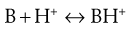 (3.8)
(3.8)
In solutions of most salts of strong acids or strong bases in water, such equilibria are shifted strongly to one side of the equation because these compounds are virtually completely ionized. In the case of aqueous solutions of weaker acids and bases, the degree of ionization is much more variable and indeed, as will be seen, controllable.
The ionization constant (or dissociation constant) Ka of a partially ionized weakly acid species can be obtained by applying the Law of Mass Action to yield Equation 3.9 in which [I+] and [I−] represent the concentrations of the dissociated ionized species and [U] is the concentration of the unionized species.
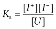 (3.9)
(3.9)
For the case of a weak acid this can be written (from Eqn 3.7) as:
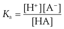 (3.10)
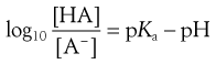
Taking logarithms of both sides of Equation 3.10 yields:
 (3.11)
The signs in this equation may be reversed to give Equation 3.12:
 (3.12)
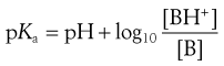
The symbol pKa is used to represent the negative logarithm of the acid dissociation constant Ka in an analogous way that pH is used to represent the negative logarithm of the hydrogen ion concentration (as Eqn 3.6). Therefore:
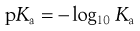 (3.13)
Now Equation 3.12 may therefore be rewritten as Equation 3.14:
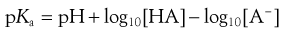 (3.14)
or
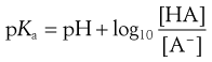 (3.15)
or even
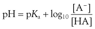 (3.16)
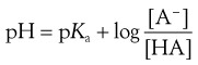
Equations 3.15 and 3.16 are known as the Henderson–Hasselbalch equations for a weak acid.
Ionization constants of both acidic and basic drugs are usually expressed in terms of pKa. The equivalent acid dissociation constant (Ka) for the protonation of a weak base is given (from Eqn 3.8) by Equation 3.17. Note the equation appears to be inverted, but it is written in terms of Ka rather than Kb (the base dissociation constant):
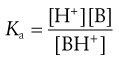 (3.17)
Taking negative logarithms yields Equation 3.18:
 (3.18)
or
 (3.19)
or
 (3.20)
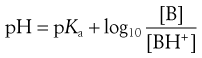
Equations 3.19 and 3.20 are known as the Henderson–Hasselbalch equations for a weak base.
Link between pH, pKa, degree of ionization and solubility of weakly acidic or basic drugs
There is a direct link for most polar ionic compounds between the degree of ionization and aqueous solubility. As has been shown above, in turn, the degree of ionization is controlled by the pKa of the molecule and the pH of its surrounding environment. This interrelationship is shown diagrammatically in Figure 3.1.
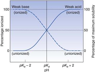
Taking the weak acid line first, it can be seen that at high pH the drug is fully ionized and at its maximum solubility. Under low pH conditions the opposite is true. The shape of the curve is defined by the Henderson–Hasselbalch equation for weak acids (Equation 3.15) that shows the link between pH, pKa and degree of ionization for a weakly acidic drug. It can also be seen from Figure 3.1 that when the pH is equal to the pKa of the drug, that drug is 50% ionized. This is also predicted from the Henderson–Hasselbalch equation.
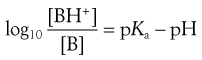
Equation 3.16 shows that when [A−] = [HA], log ([A−]/[HA]) will equal log 1 (i.e. zero) and thus pH = pKa. Put another way, when the pH of the surrounding solution equals the pKa, then the concentration of the ionized species [A−] will equal the concentration of the unionized species [HA], i.e. the drug is 50% ionized. The Henderson–Hasselbalch equations also show that a drug is almost completely ionized or non-ionized (as appropriate) when two pH units away from its pKa.
Examination of the equivalent line for a weak base will indicate that it is probably not a coincidence that most drugs for peroral delivery are weak bases. A weak base will be ionized and at its most soluble in the acidic stomach and non-ionized and therefore will be more easily absorbed in the more alkaline small intestine. The choice of the pKa for a drug is thus of paramount importance in peroral drug delivery.
Use of the Henderson–Hasselbalch equations to calculate degree of ionization of weakly acidic or basic drugs
Various analytical techniques, e.g. spectrophotometric and potentiometric methods, may be used to determine ionization constants, but the temperature at which the determination is performed should be specified because the values of the constants vary with temperature.
The degree of ionization of a drug in a solution can be calculated from rearranged Henderson–Hasselbalch equations for weak acids and bases (Eqns 3.15 and 3.19, respectively) if the pKa value of the drug and the pH of the solution are known. The resulting equations for weak acids and weak bases are Equations 3.21 and 3.22, respectively:
 (3.21)
 (3.22)
Such calculations are particularly useful in determining the degree of ionization of drugs in various parts of the gastrointestinal tract and in the plasma. The following examples are therefore related to this type of situation.
Box 3.1 Worked examples
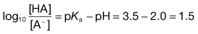
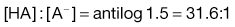
1. The pKa value of aspirin, which is a weak acid, is about 3.5. If the pH of the gastric contents is 2.0 then from Equation 3.21:
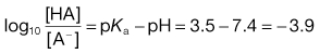
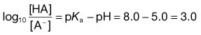
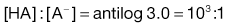
2. The pH of plasma is 7.4 so that the ratio of unionized : ionized aspirin in this medium is given by:

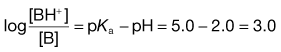
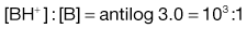
4. The pKa of the basic drug amidopyrine is 5.0. In the stomach, the ratio of ionized : unionized drug is calculated from Equation 3.22 as follows:
while in the intestine, the ratio is given by:

Buffer solutions and buffer capacity
Buffer solutions will maintain a constant pH even when small amounts of acid or alkali are added to the solution. Buffers usually contain mixtures of a weak acid and one of its salts, although mixtures of a weak base and one of its salts may be used. The latter suffer from the disadvantage that arises from the volatility of many bases.
The action of a buffer solution can be appreciated by considering, as an example, a simple system such as a solution of a mixture of acetic acid and sodium acetate in water. The acetic acid, being a weak acid, will be confined virtually to its undissociated form because its ionization will be suppressed by the presence of common acetate ions produced by complete dissociation of the sodium salt. The pH of this solution can be described by Equation 3.23, which is Equation 3.16 in which [A−] is the concentration of acetate ions and [HA] is the concentration of acetic acid in the buffer solution:
 (3.23)
It can be seen from Equation 3.23 that the pH will remain constant as long as the logarithm of the ratio [acetate]/[acetic acid] does not change. When a small amount of an acid is added to the solution, it will convert some of the salt into acetic acid, but if the concentrations of both acetate ion and acetic acid are reasonably large then the effect of the change will be negligible and the pH will remain constant. Similarly, the addition of a small amount of base will convert some of the acetic acid into its salt form but the pH will be virtually unaltered if the overall changes in concentrations of the two species are relatively small.
If large amounts of acid or base are added to a buffer, then changes in the ratio of ionized to unionized species become appreciable and the pH will then alter. The ability of a buffer to withstand the effects of acids and bases is an important property from a practical point of view. This ability is expressed in terms of buffer capacity (β). It can be defined as being equal to the amount of strong acid or strong base, expressed as moles of H+ or OH− ion, required to change the pH of 1 litre of the buffer by 1 pH unit. From the remarks above, it should be clear that buffer capacity increases as the concentrations of the buffer components increase. In addition, the capacity is also affected by the ratio of the concentrations of weak acid and its salt, maximum capacity (βmax) being obtained when the ratio of acid to salt = 1, i.e. pH equals the pKa of the acid.
The components of various buffer systems and the concentrations required to produce different pHs are listed in several reference books, such as the pharmacopoeias. When selecting a suitable buffer, the pKa value of the acid should be close to the required pH and the compatibility of its components with other ingredients in the system should be considered. The toxicity of buffer components must also be taken into account if the solution is to be used for medicinal purposes.
Colligative properties
When a non-volatile solute is dissolved in a solvent, certain properties of the resultant solution are largely independent of the nature of the solute and are determined by the concentration of solute particles. These properties are known as colligative properties. In the case of a nonelectrolyte the solute particles will be molecules,but if the solute is an electrolyte, then its degree of dissociation will determine whether the particles will be ions only or a mixture of ions and undissociated molecules.
The most important colligative property from a pharmaceutical aspect is referred to as osmotic pressure. However, since all colligative properties are related to each other by virtue of their common dependency on the concentration of the solute molecules, other colligative properties (which include lowering of vapour pressure of the solvent, elevation of its boiling point and depression of its freezing point) are of pharmaceutical interest. Observations of these other properties offer alternatives to osmotic pressure measurements as methods of comparing the colligative properties of different solutions.
Osmotic pressure
The osmotic pressure of a solution is the external pressure that must be applied to the solution in order to prevent it being diluted by the entry of solvent via a process that is known as osmosis. This is the spontaneous diffusion of solvent from a solution of low solute concentration (or a pure solvent) into a more concentrated one through a semi-permeable membrane. Such a membrane separates the two solutions and is permeable only to solvent molecules (i.e. not solute ones).
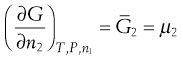
Since the process occurs spontaneously at constant temperature and pressure, the laws of thermodynamics indicate that it will be accompanied by a decrease in the free energy (G) of the system. This free energy may be regarded as the energy available for the performance of useful work. When an equilibrium position is attained then there is no remaining difference between the energies of the states that are in equilibrium. The rate of increase in free energy of a solution caused by an increase in the number of moles of one component is termed the partial molar free energy ( ) or chemical potential (µ) of that component. For example, the chemical potential of the solvent in a binary solution is given by Equation 3.24. The subscripts outside the bracket on the left-hand side indicate that temperature, pressure and amount of component 1 (the solute in this case) remain constant:
 (3.24)
Since (by definition) only solvent molecules can pass through a semi-permeable membrane, the driving force for osmosis arises from the inequality of the chemical potentials of the solvent on opposing sides of the membrane. Thus the direction of osmotic flow is from the dilute solution (or pure solvent), where the chemical potential of the solvent is highest because of the higher concentration of solvent molecules, into the concentrated solution, where the concentration and consequently the chemical potential of the solvent are reduced by the presence of more solute. The chemical potential of the solvent in the more concentrated solution can be increased by forcing its molecules closer together under the influence of an externally applied pressure. Osmosis can be prevented by such means, hence the term osmotic pressure.
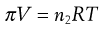
The relationship between osmotic pressure (π) and concentration of a non-electrolyte is defined for dilute solutions, which may be assumed to exhibit ideal behaviour, by the van’t Hoff equation (Eqn 3.25):
 (3.25)
where V is the volume of solution, n2 is the number of moles of solute, T is the absolute temperature and R is the gas constant. This equation, which is similar to the ideal gas equation, was derived empirically but it does correspond to a theoretically derived equation if approximations based on low solute concentrations are taken into account.
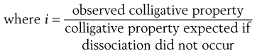
If the solute is an electrolyte, Equation 3.25 must be modified to allow for the effect of ionic dissociation, because this will increase the number of particles in the solution. This modification is achieved by insertion of the van’t Hoff correction factor (i) to give:
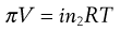 (3.26)
Osmolality and osmolarity
The amount of osmotically active particles in a solution is sometimes expressed in terms of osmoles or milliosmoles. These osmotically active particles may be either molecules or ions. Osmole values depend on the number of particles dissolved in a solution, regardless of charge. For substances that maintain their molecular structure when they dissolve (e.g. glucose), osmolarity and the molarity are essentially the same. For substances that dissociate when they dissolve, the osmolarity is the number of free particles times the molarity. Thus a 1 molar solution of pure NaCl solution would be 2 osmolar (1 for Na+ and 1 for Cl−).
The concentration of a solution may therefore be expressed in terms of its osmolarity or its osmolality. Osmolarity is the number of osmoles per litre of solution and osmolality is the number of osmoles per kilogram of solvent.
Isoosmotic solutions
If two solutions are separated by a perfect semi-permeable membrane, i.e. a membrane which is permeable only to solvent molecules, and no net movement of solvent occurs across the membrane, then the solutions are said to be isoosmotic and have equal osmotic pressures.
Isotonic solutions
Biological membranes do not always function as perfect semi-permeable membranes and some solute molecules in addition to water are able to pass through them. If two isoosmotic solutions remain in osmotic equilibrium when separated by a biological membrane, they may be described as being isotonic with respect to that particular membrane.
Adjustment of isotonicity is particularly important for formulations intended for parenteral routes of administration (this is discussed in Chapter 36). Excessively hypotonic or hypertonic solutions can cause biological damage.
Diffusion in solution
The components of a solution, by definition, form a homogeneous single phase. This homogeneity arises from the process of diffusion, which occurs spontaneously and is consequently accompanied by a decrease in the free energy (G) of the system. Diffusion may be defined as the spontaneous transference of a component from a region in the system which has a high chemical potential into a region where its chemical potential is lower. Although such a gradient in chemical potential provides the driving force for diffusion, the laws that describe this phenomenon are usually expressed, more conveniently, in terms of concentration gradients. An example is Fick’s First Law which is discussed in Chapter 2.
The most common explanation of the mechanism of diffusion in solution is based on the lattice theory of the structure of liquids. Lattice theories postulate that liquids have crystalline or quasicrystalline structures. The concept of a crystal type of lattice is only intended to provide a convenient starting point and should not be interpreted as a suggestion that liquids possess rigid structures. The theories also postulate that a reasonable proportion of the volume occupied by the liquid is, at any moment, empty, i.e. there are ‘holes’ in the liquid lattice network, which constitute the so-called free volume of the liquid.
Diffusion can therefore be regarded as the process by which solute molecules move from hole to hole within a liquid lattice. In order to achieve such movement, a solute molecule must acquire sufficient kinetic energy at the right time so that it can break away from any bonds that tend to anchor it in one hole and then jump into an adjacent hole. If the average distance of each jump is δ cm and the frequency with which the jumps occur is ϕ s−1 then the diffusion coefficient (D) is given by:
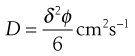 (3.27)
The diffusion coefficient is assumed to have a constant value for a particular system at a given temperature. This assumption is only strictly true at infinite dilution and the value of D may therefore exhibit some concentration dependency. In a given solvent, the value of D decreases as the size of the diffusing solute molecule increases. In water, for example, D is of the order of 2 × 10⁻⁵ cm2 s−1 for solutes with molecular weights of approximately 50 Da and it decreases to about 1 × 10⁻⁶ cm2 s−1 for molecular weight of a few thousand Da.
The value of δ for any given solute is reasonably constant. Differences in the diffusion coefficient of a substance in solution in various solvents arise mainly from changes in jump frequency (ϕ), which is determined, in turn, by the free volume or looseness of packing in the solvent.
When the size of the solute molecules is not appreciably larger than that of the solvent molecules, then it has been shown that the diffusion coefficient of the former is related to its molecular weight (M) by the relationship:
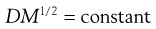 (3.28)
When the solute is much greater in size than the solvent, diffusion arises largely from transport of solvent molecules in the opposite direction and the relationship becomes:
 (3.29)
This latter equation forms the basis of the Stokes–Einstein equation (Eqn 3.30) for the diffusion of spherical particles that are larger than surrounding liquid molecules. Since the mass (m) of a spherical particle is proportional to the cube of its radius (r), i.e. r ∝ m1/3, it follows from Equation 3.29 that Dm1/3 and consequently D and r are constants for such a system. The Stokes–Einstein equation is usually written in the form:
 (3.30)
where k is the Boltzmann constant, T is the absolute temperature and η is the viscosity of the liquid. The appearance of a viscosity term in this type of equation is not unexpected because the reciprocal of viscosity, which is known as the fluidity of a liquid, is proportional to the free volume in a liquid. Thus, jump frequency (ϕ) and diffusion coefficient (D) will increase as the viscosity of a liquid decreases or as the number of ‘holes’ in its structure increases.
The experimental determination of diffusion coefficients of solutes in liquid solvents is not easy because the effects of other factors that may influence the movement of solute in the system, e.g. temperature and density gradients, mechanical agitation and vibration, must be eliminated.
Summary
This chapter has outlined the key fundamental issues relating to the properties of solutions. The issues discussed are of relevance both to dosage forms, which themselves comprise solutions, and to the fate of the drug molecule once in solution following administration.
Bibliography
1. Banker GS, Rhodes CT. Modern Pharmaceutics. 4th edn New York: Marcel Dekker; 2002.
2. Cairns D. Essentials of Pharmaceutical Chemistry. 4th edn London: Pharmaceutical Press; 2012.
3. Chang R. Physical Chemistry with Applications to Biological Systems. 2nd edn Basingstoke: Macmillan; 1981.
4. Florence AT, Attwood D. Physicochemical Principles of Pharmacy. 5th edn London: Pharmaceutical Press; 2011.
5. Martin A, Bustamante P. Physical Pharmacy: Physical Chemical Principle in the Pharmaceutical Sciences. 4th edn Philadelphia, USA: Lea and Febiger; 1993.
6. Troy DB, ed. Remington: The Science and Practice of Pharmacy. 21st edn Maryland, USA: Lippincott, Williams and Wilkins; 2006.
[/level-membership-for-basic-science-category][not-level-membership-for-basic-science-category]
Properties of solutions
Michael E. Aulton
Chapter contents
Vapour pressures of solids, liquids and solutions
Hydrogen ion concentration and pH
Dissociation (or ionization) constants; pKa and pKb
Key points
Introduction
The aim of this chapter is to provide information on certain properties of solutions that relate to their applications in pharmaceutical science. This chapter deals mainly with the physicochemical properties of solutions that are important with respect to pharmaceutical systems. These aspects are covered in sufficient detail to introduce the pharmaceutical scientist to these properties to allow an understanding of their importance in dosage form design and drug delivery. Much is published elsewhere in far greater detail and any reader requiring this additional information can trace some of this by referring to the bibliography at the end of the chapter.
Types of solution
Solutions may be classified based on the physical state (i.e. gas, liquid or solid) of the solute(s) and solvent. Although a variety of different types can exist, solutions of pharmaceutical interest virtually all possess liquid solvents. In addition, the solutes are predominantly solid substances. Consequently, most of the information in this chapter is relevant to solutions of solids in liquids.
Vapour pressures of solids, liquids and solutions
An understanding of many of the properties of solutions requires an appreciation of the concept of an ideal solution and its use as a reference system, to which the behaviours of real (non-ideal) solutions can be compared. This concept is itself based on a consideration of vapour pressure. The present section serves as an introduction to the later discussions on ideal and non-ideal solutions.
The kinetic theory of matter indicates that the thermal motion of molecules of a substance in its gaseous state is more than adequate to overcome the attractive forces that exist between the molecules. Thus, the molecules will undergo a completely random movement within the confines of the container. The situation is reversed, however, when the temperature is lowered sufficiently so that a condensed phase is formed. Here the thermal motions of the molecules are now insufficient to overcome completely the intermolecular attractive forces and some degree of order in the relative arrangement of molecules occurs. This condensed state may be either liquid or solid.
If the intermolecular forces are so strong that a high degree of order is brought about, when the structure is hardly influenced by thermal motions, then the substance is usually in the solid state.
In the liquid condensed state, the relative influences of thermal motion and intermolecular attractive forces are intermediate between those in the gaseous and solid states. Thus, the effects of interactions between the permanent and induced dipoles, i.e. the so-called van der Waals forces of attraction, lead to some degree of coherence between the molecules of liquids. Consequently, liquids occupy a definite volume with a surface, unlike gases, and whilst there is evidence of structure within liquids, such structure is much less apparent than in solids.
Although both solids and liquids are condensed systems with cohering molecules, some of the surface molecules in these systems will occasionally acquire sufficient energy to overcome the attractive forces exerted by adjacent molecules. The molecules can therefore escape from the surface to form a vapour phase. If temperature is maintained constant, equilibrium will be established eventually between the vapour phase and the condensed phase. The pressure exerted by the vapour at this equilibrium is referred to as the vapour pressure of the substance.
All condensed systems have the inherent ability to give rise to a vapour pressure. However, the vapour pressures exerted by solids are usually much lower than those exerted by liquids, because the intermolecular forces in solids are stronger than those in liquids. Thus, the escaping tendency for surface molecules is higher in liquids. Consequently, surface loss of vapour from liquids by the process of evaporation is more common than surface loss of vapour from solids by sublimation.
In the case of a liquid solvent containing a dissolved solute, molecules of both solvent and solute may show a tendency to escape from the surface and so contribute to the vapour pressure. The relative tendencies to escape will depend on the relative numbers of the different molecules in the surface of the solution, and on the relative strengths of the attractive forces between adjacent solvent molecules on the one hand and between solute and solvent molecules on the other hand. Because the intermolecular forces between solid solutes and liquid solvents tend to be relatively strong, such solute molecules do not generally escape from the surface of a solution nor contribute to the vapour pressure. In other words, the solute is generally non-volatile and the vapour pressure arises solely from the dynamic equilibrium that is set up between the rates of evaporation and condensation of solvent molecules contained in the solution. In a mixture of miscible liquids, i.e. a liquid in liquid solution, the molecules of both components are likely to evaporate and contribute to the overall vapour pressure exerted by the solution.
Ideal solutions: Raoult’s Law
The concept of an ideal solution has been introduced in order to provide a model system that can be used as a standard to which real or non-ideal solutions can be compared. In the model, it is assumed that the strengths of all intermolecular forces are identical. Thus solvent/solvent, solute/solvent and solute/solute interactions are the same and are equal to the strength of the intermolecular interactions in either the pure solvent or pure solute. Because of this equality, the relative tendencies of solute and solvent molecules to escape from the surface of the solution will be determined only by their relative numbers in the surface.
Since a solution is homogeneous by definition, then the relative number of these surface molecules will be the same as the relative number in the whole of the solution. The latter can be expressed conveniently by the mole fractions of the components because, for a binary solution (i.e. one with two components), x1 + x2 = 1, where x1 and x2 are the mole fractions of the solute and solvent, respectively.
The total vapour pressure (P) exerted by a binary solution is given by Equation 3.1:
(3.1)
where p1 and p2 are the partial vapour pressures exerted above the solution by the solute and solvent, respectively. Raoult’s Law states that the partial vapour pressure (p) exerted by a volatile component in a solution at a given temperature is equal to the vapour pressure of the pure component at the same temperature (po) multiplied by its mole fraction in the solution (x), i.e.:
(3.2)
Thus from Equations 3.1 and 3.2:
(3.3)
where and are the vapour pressures exerted by pure solute and pure solvent, respectively. If the total vapour pressure of the solution is described by Equation 3.3, then Raoult’s Law is obeyed by the system.
One of the consequences of the preceding comments is that an ideal solution may be defined as one that obeys Raoult’s Law. In addition, ideal behaviour should be expected to be exhibited only by real systems composed of chemically similar components, because it is only in such systems that the condition of equal intermolecular forces between components (as assumed in the ideal model) is likely to be satisfied. Consequently, Raoult’s Law is obeyed over an appreciable concentration range by relatively few systems in reality.
Mixtures of, for example, benzene + toluene, n-hexane + n-heptane, ethyl bromide + ethyl iodide and binary mixtures of fluorinated hydrocarbons are systems that exhibit ideal behaviour. Note the chemical similarity of the two components of the mix in each example.
Real or non-ideal solutions
The majority of real solutions do not exhibit ideal behaviour because solute–solute, solute–solvent and solvent–solvent forces of interaction are unequal. These inequalities alter the effective concentration of each component so that it cannot be represented by a normal expression of concentration, such as the mole fraction term x that is used in Equations 3.2 and 3.3. Consequently, deviations from Raoult’s Law are often exhibited by real solutions and the previous equations are not obeyed in such cases. These equations can be modified, however, by substituting each concentration term (x) by a measure of the effective concentration; this is provided by the so-called activity (or thermodynamic activity), a. Thus, Equation 3.2 is converted into Equation 3.4:
(3.4)
and the resulting equation is applicable to all systems whether they are ideal or non-ideal. It should be noted that if a solution exhibits ideal behaviour then a equals x, whereas a will not equal x if deviations from such behaviour are apparent. The ratio of activity divided by the mole fraction is termed the activity coefficient (f) and it provides a measure of the deviation from the ideal. Thus when a = x, f = 1.
If the attractive forces between solute and solvent molecules are weaker than those between the solute molecules themselves or between the solvent molecules themselves, then the components will have little affinity for each other. The escaping tendency of the surface molecules in such a system is increased when compared with an ideal solution. In other words, p1, p2 and therefore P are greater than expected from Raoult’s Law and the thermodynamic activities of the components are greater than their mole fractions, i.e. a1 > x1 and a2 > x2. This type of system is said to show a positive deviation from Raoult’s Law and the extent of the deviation increases as the miscibility of the components decreases. For example, a mixture of alcohol and benzene shows a smaller deviation than the less miscible mixture of water + diethyl ether whilst the virtually immiscible mixture of benzene + water exhibits a very large positive deviation.
Conversely, if the solute and solvent molecules have a strong mutual affinity (that sometimes may result in the formation of a complex or compound), then a negative deviation from Raoult’s Law occurs. Thus, p1, p2 and therefore P are lower than expected and a1 < x1 and a2 < x2. Examples of systems that show this type of behaviour include chloroform + acetone, pyridine + acetic acid and water + nitric acid.
Although most systems are non-ideal and deviate either positively or negatively from Raoult’s Law, such deviations are small when a solution is dilute. This is because the effect that a small amount of solute has on interactions between solvent molecules is minimal. Thus, dilute solutions tend to exhibit ideal behaviour and the activities of their components approximate to their mole fractions, i.e. a1 approximately equals x1 and a2 approximately equals x2. Conversely, large deviations may be observed when the concentration of a solution is high.
Knowledge of the consequences of such marked deviations is particularly important in relation to the distillation of liquid mixtures. For example, the complete separation of the components of a mixture by fractional distillation may not be achievable if large positive or negative deviations from Raoult’s Law give rise to the formation of so-called azeotropic mixtures with minimum and maximum boiling points, respectively.
Ionization of solutes
[/not-level-membership-for-basic-science-category]
