[level-membership-for-hematology-oncology-and-palliative-medicine-category]
7 Principles of Radiation Physics
In this chapter, we present the basic radiation physics needed for the practice of radiation oncology. Many of the specific applications of these basic physics principles, such as brachytherapy and treatment planning, are presented elsewhere in this textbook. Since the primary audience for this textbook is assumed to be practicing radiation oncologists and resident clinicians, many topics are not treated in the detail that would be required by radiation physicists. Excellent physics textbooks that present the topics in more depth are available.1–4
Basic Concepts
Atomic and Nuclear Structure
 . Isotopes of an element have the same Z but different A and, therefore, have the same chemical properties but can have different physical properties. Isobars are atoms with the same A but different Z, and isotones are atoms with different A and Z but the same N.
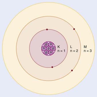
In the planetary model of the atom, first described by Niels Bohr, the electron orbits make up discrete concentric shells, with a different binding energy associated with each shell. The shells are labeled K, L, M, and so on from the innermost to the outermost shell. The maximum number of electrons allowed in each shell is 2n2, where n = 1 for the K shell, n = 2 for the L shell, and so on. Therefore, there are up to 2 electrons in the K shell, 8 in the L shell, 18 in the M shell, and so on. A simple schematic drawing of the Bohr model is shown in Fig. 7-1.
Nuclear Transformations
The explanation of nuclear decay depends on understanding the interplay between the very strong, attractive nuclear force that binds the neutrons and protons together in the nucleus, and the moderately strong repulsive electromagnetic force between the protons. As the protons and neutrons move about within the nucleus, there is some probability that one of them will acquire enough kinetic energy to escape from the nuclear potential energy “well.” Large nuclei with many neutrons and protons tend to be less stable because of the increasing repulsion of the protons. For large nuclei to be stable, an excess of neutrons is required to provide the nuclear attraction to keep the protons from escaping. Fig. 7-2 shows the line of stable nuclei for the range of known elements.
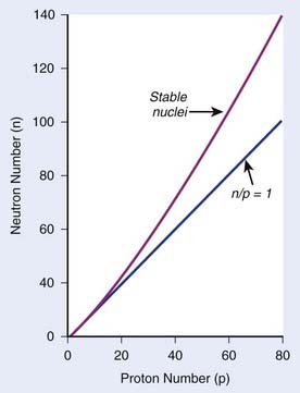
FIGURE 7-2 • Plot of numbers of neutrons and protons in stable nuclei.
(From Khan FM: The physics of radiation therapy, ed 3, Philadelphia, 2003, Lippincott Williams & Wilkins, p 4.)
Decay Constant
where N is the number of radioactive nuclei and λ is the decay constant. The minus sign indicates that the number of nuclei is decreasing with time. Integration of this differential equation leads to the following equation:
where N0 is the number of radioactive nuclei initially present, N(t) represents the number remaining at time t, and e is the base of the natural logarithm (2.71828).
where A0 is the initial activity and A(t) is the activity at time t. The unit of activity is the Curie (Ci) or the Becquerel (Bq), which is 1 disintegration per second:

Half-Life and Mean Life
the mean or average life (Tλ) is the time for the number of atoms to decay to 1/e of the initial number, so
Radioactive Decay Series and Equilibrium
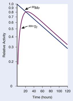
In each series, the half-life of the parent is longer than any of the half-lives of any of the daughter nuclides. This phenomenon leads to a state of transient or secular equilibrium. Since each daughter is less stable than the original parent, the activity of the daughter will increase with time, until it approaches the activity of the long-lived parent. If the half-lives are very different, the activities will become essentially identical after a number of daughter half-lives, and this is called secular equilibrium. An example is shown in Fig. 7-3. If the half-lives of the parent and daughter are very similar, transient equilibrium is reached in a few half-lives, after which the daughter has an activity in excess of the parent activity but decays with the same rate as the limiting parent decay rate. An example of this phenomenon is shown in Fig. 7-4. For either case, after a time that is long compared to the half-life of the shorter-lived nuclide,
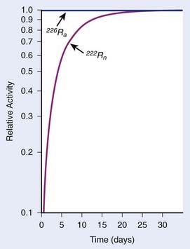
FIGURE 7-3 • Example of secular equilibrium in the decay of 226Ra to 222Rn.
(From Khan FM: The physics of radiation therapy, ed 3, Philadelphia, 2003, Lippincott Williams & Wilkins, p 19.)
where Ai and Ti refer to the activity and half-life of the daughter (d) or parent (p).
X-Ray Production
Characteristic X-Rays
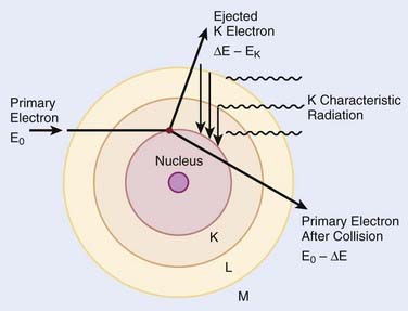
When electrons are incident on target atoms, they can ionize those atoms by depositing sufficient energy to eject an inner shell electron. The inner shell vacancy is subsequently filled by an outer shell electron, causing the emission of a characteristic x-ray with energy equal to the difference between the binding energies of the inner and outer shells. This process is diagrammed in Fig. 7-5. Although this process can take place in both low-Z and high-Z atoms, only for high-Z atoms are the binding energies sufficient to produce radiation in the x-ray portion of the electromagnetic spectrum. For example, the binding energy of K-shell electrons in tungsten, a common target for x-ray tubes and accelerators, is about 70 keV, whereas for aluminum, it is only about 1.5 keV. As mentioned earlier, the characteristic x-ray energy is occasionally transferred directly to an orbital electron, leading to the production of an Auger electron.
Bremsstrahlung X-Rays
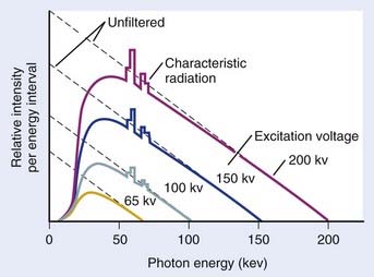
In general, both bremsstrahlung and characteristic x-rays are present when electrons strike a target. Fig. 7-6 shows x-ray spectra for a thick tungsten target for electron energies of from 65 keV to 200 keV. Note the appearance of the characteristic x-rays on top of the bremsstrahlung spectrum once the electron energy is in excess of the K-shell binding energy of 70 keV. Any material in the x-ray beam, including the target itself, will absorb some of the energy of the beam. The effect of such absorption is to preferentially filter out the low energy portion of the bremsstrahlung spectrum. The process of preferentially attenuating the low-energy component of the beam is referred to as “beam hardening.” When the beam is hardened, the average energy of the x-rays increases at the expense of reduced intensity.
Interaction of X-Rays and Particles With Matter
X-Ray Interactions
where dN is the reduction in the number of photons due to interactions in a thickness dx of an absorber, N is the number of incident photons, and µi is the attenuation coefficient for the ith interaction process. After integration over the thickness, this equation becomes
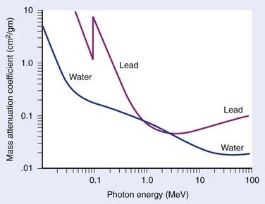
where N(x) is the number of photons left in the beam (without interaction) as a function of the thickness x of material traversed, and µtot is the sum of the individual attenuation coefficients. (µi/ρ) is called the mass-attenuation coefficient for process i, where ρ is the density of the material. Dividing the conventional attenuation coefficients by density removes the dependence on the physical density of materials and the resulting mass attenuation coefficients are approximately equal from material to material. The corresponding thickness, ρx, is in units of grams per square centimeter (g/cm2). The total mass attenuation coefficients for water and lead are shown as functions of energy in Fig. 7-7. There are five different photon interaction processes, including coherent scattering, photoelectric effect, Compton scattering, pair production, and photodisintegration. These will be discussed in turn.
implying that
Compton Scattering
Compton scattering is a process in which the incident photon interacts with an orbital electron as if it were a free particle, since the binding energy is small compared to the photon energy. The dynamics of the interaction can be described as a typical particle–particle scattering interaction whereby the photon transfers some of its energy to the electron and is scattered at an angle φ relative to the incident direction. The electron is ejected at an angle θ relative to the forward direction. The energy of the outgoing Compton-scattered photon is equal to the difference between the incident photon energy and the energy transferred to the electron. A diagram of the Compton process is shown in Fig. 7-8.
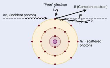
FIGURE 7-8 • Illustration of the Compton effect.
(From Khan FM: The physics of radiation therapy, ed 3, Philadelphia, Lippincott Williams & Wilkins, p 67.)
From conservation of momentum:
and
where ve is the velocity of the electron, me is the rest mass of the electron, c is the speed of light, and
Solving these three simultaneous equations, we obtain the following relationships:
where α = hνo/ mec2 and f = (1 − cos φ).
Relative Importance of Interaction Types
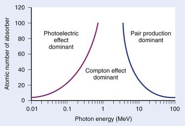
The total mass absorption coefficient is the sum of the coefficients for coherent, photoelectric, Compton, and pair production. For low-Z targets such as tissue (average Z = 7), Compton processes are overwhelmingly dominant throughout the range of energies used in therapy. Fig. 7-9 shows the relative importance of photoelectric, Compton, and pair production as a function of photon energy and the atomic number of the target material.4 For tissue, Compton dominates between approximately 30 keV and 30 MeV, whereas for lead, photoelectric dominates up to approximately 800 keV and pair production above about 5 MeV. Because of its calcium content, bone has a higher absorption by photoelectric and pair production. This leads to high bone doses for orthovoltage and kilovoltage and for higher energy accelerator beams.
Charged Particles
Electrons
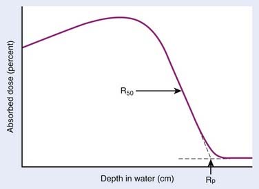
Electrons lose energy to the medium by two processes, ionization and radiation. Ionization processes are interactions with the atomic electrons, whereas radiation losses are interactions with the field of the nucleus, leading to bremsstrahlung x-ray production. Whereas the microscopic interactions are well understood, the macroscopic description of the energy and range of the particles at any point in the medium is not simple. This is because the electrons are very much lighter than the atomic nuclei. Therefore, the electron can lose a very large fraction of its energy in a single process and can be deflected by very large angles. This means that even if the electron beam is monoenergetic when entering a medium, there will be a large amount of range-straggling, or a large variation from electron to electron as to where, in the phantom, the electron will stop. Fig. 7-10 shows a plot of absorbed dose as a function of depth for monoenergetic electrons incident on water. There is a depth beyond which the dose is almost zero, where all the incident electrons have been stopped and where the remaining dose is due to bremsstrahlung x-rays produced by the electrons in the medium. This is in sharp contrast to the exponential falloff of dose for x-rays. This ranging out of electrons in matter is responsible for the popularity of electrons for treatment of superficial disease.
Protons and Heavier Ions
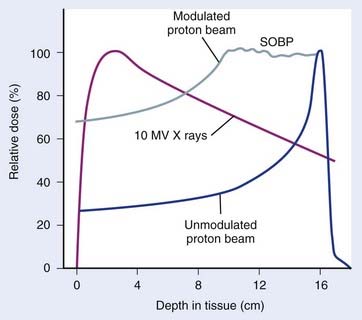
The use of protons and heavy ions for radiotherapy was pioneered in the 1970s and 1980s at the Massachusetts General Hospital in collaboration with the now decommissioned Harvard Cyclotron Laboratory and at the Lawrence Berkeley National Laboratory in Berkeley, California.5–15 Since then, several proton and charged-particle facilities have been built around the world, a list of which can be found on the website for the Particle Therapy Co-Operative Group (PTCOG; http://ptcog.web.psi.ch/). Similar to electrons, protons lose energy primarily by electromagnetic interactions with the atomic electrons. A major difference between protons and electrons is that protons are much heavier than electrons and therefore lose only a very small fraction of their energy in an individual interaction, scattering minimally in the process. Protons lose energy at an increasing rate as they slow down, yielding an enhanced region of energy deposition called the Bragg Peak just before they stop. One can predict very accurately the depth at which the protons will come to rest if the initial energy of the protons and the electron density of the material traversed are known. The absence of exit dose beyond the intended target makes protons nearly ideally suited for optimal physical dose delivery. A typical depth dose distribution for a clinical, energy-modulated proton beam, compared to that of a 10-MV bremsstrahlung x-ray beam, is shown in Fig. 7-11. A small percentage of proton interactions is via nuclear interactions with the nucleus. These rare interactions are qualitatively different than electromagnetic interactions and are thought to be responsible for enhancing the cell kill per unit dose by about 10% to 20% over that of x-rays.16
Heavy ions such as helium, carbon, neon, and argon nuclei have also been used in radiotherapy.9–12,14,15,17,18 Similar to protons, they lose energy by interacting with the atomic electrons. Being even heavier than protons, they scatter even less and have even more rapid dose falloff outside the central beam and even faster falloff of dose beyond the end of range. In addition to these electromagnetic interactions, heavy ions have a probability of interacting with the nucleus via nuclear interactions that increases with the mass of the incident ion. In particular, as the heavy ions begin to slow down, they tend to suffer nuclear interactions in which they lose a very large amount of their energy in a single event. This high density of deposited energy kills cells in a far more efficient way per unit dose than x-rays. These particles are said to have a high radiobiologic efficiency (RBE). For more information on these particles, the reader is referred to the literature.13
Neutrons
Neutrons have also been used in clinical treatments.19–24 These particles are neutral, so they cannot lose energy by any means other than the nuclear interaction. All of their interactions are “catastrophic,” because a significant portion of their energy is deposited in an individual event. Their primary interactions are with protons within the nucleus. These nuclear events result in recoil protons and charged nuclear fragments that have rather low energy and deposit large amounts of energy very close to the site of the original interaction. The falloff of neutron dose with depth is exponential and similar to that of low-energy x-rays, with the depth of the 50% dose being around 10 cm for typical treatment energies. Neutrons are very efficient in producing cell kill per unit dose (high RBE) relative to x-rays for both tumor tissue and normal tissues. Clinical trials have been conducted to investigate the areas where neutrons might have an advantage over x-rays. A summary of the physical characteristics and results of early clinical results is available.13
In addition, clinical trials are under way to investigate the use of slow neutrons, either thermal or epithermal in energy, to treat boronated tumor cells in patients.25–32 The clinical efficacy of these neutrons for cancer therapy depends on the very high cross section for neutron capture by boron and on a high ratio of boron in the tumor cells to that in the surrounding normal cells. To date, clinical results of these trials have been disappointing.
Radiation Therapy Treatment Machines
Kilovoltage Units
A schematic diagram of an x-ray tube suitable for radiation therapy is shown in Fig. 7-12. Since a high-voltage supply is used to generate the accelerating potential for the electron beams, a maximum energy of approximately 300 kV is achievable with this design. The resulting x-ray beams have a spectrum of photon energies with a maximum equal to the energy of the electron beam.
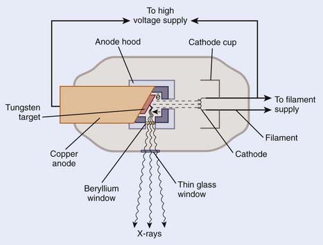
FIGURE 7-12 • Schematic diagram of an x-ray tube that could be used for radiation therapy.
(From Khan FM. The physics of radiation therapy, ed 3, Philadelphia, Lippincott Williams & Wilkins, p 29.)
Megavoltage Units
X-ray and γ-ray beams of energy greater than 1 MV are classified as megavoltage beams. In the 1930s a number of transformer-based and van de Graaff generator–based units working in the 800 KeV to 2 MeV range were installed around the world. However, it was not until the introduction of the 60Co teletherapy machine and the linear accelerator that the routine use of megavoltage x-ray and γ-ray beams occurred, significantly changing the practice of radiotherapy and leading to substantial improvements in clinical results.33
Teletherapy Machines
The megavoltage era began with the introduction of the 60Co teletherapy machine into radiotherapy clinics beginning in 1951.34,35 The development of nuclear reactors in the late 1940s made possible the production of small 60Co sources with specific activities (in Curies per gram) high enough to produce clinically acceptable dose rates of more than 1 Gray (Gy) per minute at a typical treatment distance of 80 cm from the source. These machines quickly became the standard of radiotherapy because of their simplicity of design and operation, low cost, and availability. The two photons produced by the decay of 60Co have energies of 1.17 and 1.33 MeV, yielding a depth-dose curve that falls to 50% of maximum in about 10 cm of water or tissue. In addition, the relatively high energy of the photons leads to “skin sparing” due to a reduced entrance dose that builds up for a distance of 5 mm (the maximum range of the secondary electrons from 60Co photons) to a maximum value. The half-life of 60Co is 5.27 years, making the source change a relatively infrequent requirement. With the highest specific activities currently achievable, dose rates of at least 1.5 Gy per minute for a field size of 40 cm × 40 cm can be achieved at 80 cm source-to-treatment distance.
Betatrons
The next chronological development in treatment machines is the betatron, first developed by D. W. Kerst at the University of Illinois36 primarily for physics experimentation. Electrons with energies of up to 45 MeV have been produced in betatrons for radiotherapy and used either directly or to produce bremsstrahlung x-ray beams. The massive size of these machines, their high cost, and relatively low dose rate combined to limit their usefulness in radiation therapy.
Linear Accelerators
The use of microwaves to accelerate electrons to high energies for radiotherapy was first demonstrated in Great Britain in 1953.37 This became possible primarily because of the development of high-power microwave generators for military radar use during World War II. The major components of a typical medical linear accelerator (linac) are shown in a block diagram in Fig. 7-13. The acceleration of the electron beam takes place in the accelerator wave guide, consisting of a stack of cylindrical cavities with a hole through the center, into which resonant electromagnetic waves of frequency in the microwave range (∼3000 MHz) have been coupled. The electron beam is created and preaccelerated to approximately 50 keV in a conventional electrostatic electron gun, injected into the resonating waveguide, spatially bunched and accelerated through interactions with the electromagnetic field in the individual cavities, and then emerges from the accelerating structure as a narrow pencil beam that can be magnetically bent or focused onto a scattering foil (for electron treatments) or a bremsstrahlung target (for x-ray treatments) in the treatment head of the linac. For low energies of 6 MeV or less, the beam can be magnetically focused in the forward (vertical) direction onto the axis of the treatment head, whereas at higher energies, the beam is usually bent through a 90-degree or 270-degree angle before entering the treatment head since the accelerating structure is much longer for high energies and is frequently oriented horizontally to save space. For more details about the acceleration process, the reader is referred to several excellent review articles in the literature.38–40
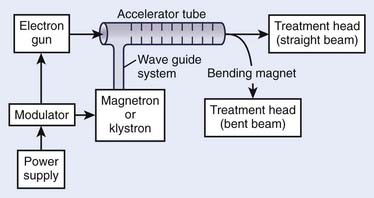
FIGURE 7-13 • A block diagram of a typical medical linear accelerator.
(From Khan FM: The physics of radiation therapy, ed 3, Philadelphia, 2003, Lippincott Williams & Wilkins, p 43.)
Although the details of the acceleration process can be quite technical, the shaping of the beam in the treatment head is both important and conceptually easy to understand. Fig. 7-14 shows a schematic diagram of the head of a typical linear accelerator in x-ray and electron treatment mode. In the x-ray mode, the beam first strikes an x-ray target made of high-Z material such as tungsten and produces a bremsstrahlung beam that is forward peaked—the higher the electron energy, the more forward the angular distribution of the resulting x-rays. After primary collimation, the beam strikes a flattening filter made of high-Z material that is thick in the center and thin toward the outside, thereby flattening the angular distribution of the x-ray beam. Although the beam can be made precisely flat only for one particular field size and at one particular depth in a patient, the filters are selected to produce beams that have acceptable flatness over the entire range of field sizes and depths normally used in therapy. If the accelerator is designed to deliver x-ray bremsstrahlung beams produced by electrons of more than one energy, a second flattening filter, optimized for that energy, will be rotated into position on the carousel. Following the flattening filter, the beam encounters the transmission ion chamber used to monitor the beam intensity (and, if segmented, the beam position), and then a secondary collimator that, along with the primary collimator, defines the rectangular field size. Patient-specific collimators and compensators, as well as wedges, if required, are placed beyond the secondary collimator as shown. In all contemporary machines dual ion chambers are used.
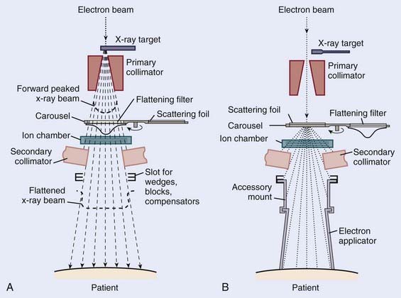
In the electron mode the x-ray target is out of position and the beam first strikes a thin scatterer that is rotated into position on the multielement carousel. This scatterer is designed to produce flat electron beams when used in combination with a field size–specific combination of secondary collimator settings and electron applicators as shown in Fig. 7-14. The scatterer is commonly a dual system of lead foils, with the second foil thicker in the center to remove the forward peaking prevalent at high energies. Bremsstrahlung x-rays will inevitably be produced in the scattering foils, but since the foils are thin, they will typically account for less than 5% of the dose received by the patient. The transmission monitor ion chamber remains in the beam as for x-ray therapy.
In the 1990s a new X-band linear accelerator was developed for medical applications. This accelerator operates at ∼9000 MHz frequency, resulting in a smaller diameter wave guide. X-band linacs capable of accelerating electrons to 6 or 12 MeV are relatively compact and are now being used with a robotic delivery system41; a portable IORT device; and a tomotherapy device, which mounts it on a computed tomography gantry.42
Microtrons
The microtron is an electron accelerator that combines the linear acceleration principle of the linac with a fixed magnetic field to confine the electrons, similar to a cyclotron (see later). The electrons move in circular orbits of increasing radii as they repeatedly recirculate through a resonant accelerating cavity. A moveable deflection tube can be placed in any location inside the magnet to select the desired electron energy for extraction. The advantages of the microtron over a linear accelerator are its simplicity, compact size, and ease of energy selection. In addition, compared to a linac, the energy spread, beam divergence, and beam size are all small, simplifying subsequent beam transport. The first example of a microtron in clinical use was a 10-MeV unit described in 1972.43 The first commercial unit, manufactured by AB Scanditronix in Sweden, was a 22 MeV unit installed at the University of Umeå, Sweden.44 Currently, microtron units of up to 50 MeV are installed at various facilities in Europe and the United States.
Cyclotrons
In its simplest form, the cyclotron is composed of two conducting D-shaped half-cylinders that are evacuated and placed between the poles of a direct current magnet. An alternating potential difference is applied between the two Ds such that when protons are injected into the center of the Ds, they are accelerated toward the negative potential. Under the constant magnetic field, they travel in circular orbits, experiencing acceleration each time they reach the gap. Energies of 200 MeV or more are needed for proton therapy if all areas of the body are to be reached. Deuteron energies of approximately 50 MeV are adequate for the production of neutron beams for therapy. Proton and deuteron beams of these energies can be produced in appropriately designed cyclotrons. Most of the accelerators in use today for proton therapy are cyclotrons.45,46
Synchrotrons
Whereas cyclotrons use a fixed magnetic field and variable radius orbits as the particles increase energy, synchrotrons use a variable magnetic field and a fixed radius orbit to confine the protons or other heavy charged particles. The synchrotron consists of a ring of magnets with interspersed resonating structures that together can confine and accelerate the charged particles to high energy. Loma Linda University Medical Center has the world’s first dedicated proton facility that uses a synchrotron to produce proton beams that are used in any of several treatment rooms.8 Synchrotrons have also been used to create heavy ion charged particle beams for radiotherapy at Lawrence Berkeley Laboratory in California and at the National Institute for Radiological Sciences in Chiba, Japan.17
Radiation Dosimetry
Radiation Exposure

Although this definition is difficult to use operationally, the free-air chamber that can directly measure exposure for photons of energy less than approximately 3 MeV has been constructed and used in standards laboratories for absolute measurements.1 The difficulty with satisfying the definition for higher energies is that the mean free path length in air for electrons produced by high energy photons is several meters, and therefore the free air chamber, which must be large enough to stop these electrons, is not practical above a few MeV. As a result, exposure is not a valid concept at energies above 3 MeV.
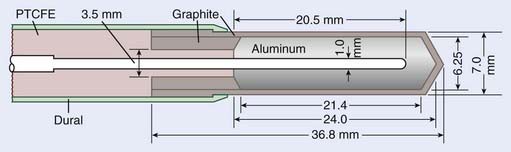
In practice, thimble ionization chambers are used to measure exposure. These chambers, either cylindrical or spherical in shape, typically contain less than 1 ml of air and, in combination with an electrometer, can be used conveniently and reproducibly to measure the quantity of charge produced when ionizing radiation passes through those volumes. National standards laboratories, using either free-air chambers or other methods, can provide calibrations of these chambers in units of R/C (i.e., exposure per unit of collected charge in a 60Co beam that can then be converted to dose per unit collected charge in beams of other energies and in phantoms of various materials). A schematic diagram of a typical cylindrical thimble ionization chamber is shown in Fig. 7-15.
Absorbed Dose
Another useful concept is kerma, an acronym for kinetic energy released in the medium. Although it has the same units as dose, the distinction is that kerma refers to energy transferred to the medium, whereas dose refers to energy absorbed by the medium. As a beam of photons enters a medium, there is an initial distance in which secondary electrons are being produced more rapidly than they are being stopped (the “buildup region”) due to the interactions of the photons with the material. In this region, the absorbed dose is increasing with depth, whereas the kerma is decreasing with depth because of the exponential attenuation of the beam in the medium. After a distance that corresponds approximately to the path length of the highest energy secondary electron that can be produced by a photon in the beam, the number of electrons produced per unit pathlength becomes approximately equal to the number that come to the end of their range. From this depth on, the photons are said to be in electronic equilibrium with the secondary electrons and kerma is approximately equal to dose. Fig. 7-16 shows the relationship between kerma and dose as a function of depth.
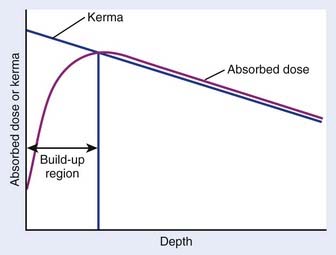
FIGURE 7-16 • Schematic plot of absorbed dose and kerma as functions of depth.
(From Khan FM: The physics of radiation therapy, ed 3, Philadelphia, 2003, Lippincott Williams & Wilkins, p 164.)
Dose Determination
Absolute dose determinations are difficult. They require a detector that responds linearly to deposited energy and that has an absolute calibration factor in units of response per unit dose that is known or that can be determined independently. Most practical dosimetry for clinical linear accelerator beams is performed with ionization chambers that are calibrated by accredited radiation laboratories whose measurements can be traced to the National Institute of Standards and Technology (NIST). These laboratories calibrate ionization chambers in one of two ways, either in terms of the absorbed-dose-to-water or in terms of the exposure in air. Before 1999 the standard practice for clinical dosimetry was to use in-air calibration factors for ionization chambers, and to apply a number of beam-specific and chamber-specific factors to convert the exposure rate in air to absorbed dose in water. One protocol used by medical physicists for doing this is called TG-21.47 More recently, a new dosimetry protocol has been introduced by the American Association of Physicists in Medicine (AAPM), which relies on the absorbed-dose-to-water as opposed to the exposure rate in air. This protocol is called TG-51,48 and in many ways is simpler to implement than TG-21.
Absolute Dose Measurements
Calorimeters
The most widely used direct dose measuring device is the calorimeter. The calorimeter can be used to determine absorbed dose by measuring a change in temperature in an irradiated material since, for most materials, energy deposited eventually appears as heat within the material, although for some materials a small portion of the absorbed energy (called the thermal defect) may be lost because of lattice deformations or chemical changes. The primary detector in the calorimeter is a thermistor embedded in the absorbing phantom. A thermistor is a solid state device that has a rapidly varying resistance with temperature. In carefully controlled situations, a thermistor can measure a change in temperature of as little as 10−5 °C. This corresponds to a deposited dose of approximately 4 cGy in water. To accurately measure clinically relevant doses delivered at achievable dose rates, the thermistor needs to be very well isolated from the outside environment so that temperature changes due to atmospheric conditions are much smaller than those produced by the energy absorbed from the beam during the time required to make a single measurement. Successful calorimeters have been constructed out of carbon,49 water,50–52 and tissue-equivalent conducting plastic.53 An excellent review of the field of calorimeters can be found in Attix’s textbook on radiation dosimetry.54 Although calorimeters are the most direct method of measuring dose, they are generally expensive, bulky, and difficult to use. Therefore, they are rarely used for routine clinical dosimetry, although water calorimetry is becoming close to a standard for calibrations laboratories worldwide.55 For example, the NIST uses water calorimetry as its standard.
Fricke Dosimetry
The Fricke dosimeter56 is based on the conversion of ferrous sulfate ions in a solution to ferric sulfate ions due to the deposition of energy by ionizing radiation. It is not truly a direct dosimeter because there is no a priori way of knowing the calibration constant in units of molecules of ferric ion produced per unit of absorbed dose. This calibration factor, called the G value, is dependent on both energy and modality. However, since the dosimeter response is proportional to absorbed dose, it can be a useful device, particularly since the solution is tissue-equivalent and the dosimeter is very small.
Exposure-Based Dosimetry
where
The corrections that must be made to obtain exposure include, most importantly, a correction for differences in temperature and pressure between the calibration condition (normally Nx is valid for a temperature of 22° C and atmospheric pressure of 760 mm Hg) and the experimental condition.1 If the walls of the chamber are assumed to be made of condensed air-equivalent material and are thick enough to produce electronic equilibrium, then the dose to the air of the chamber is obtained by multiplying the exposure by W/e, the average energy required to create an ion pair for electrons in air per unit charge collected, where W/e = 33.97 J/C:
where fmed, the term in brackets in this equation, was referred to historically as the roentgen-to-rad conversion factor.2 It must be realized that since the roentgen is only defined for energies 3 MeV or less, this exposure-based dosimetry method is also valid only in this low-energy region. The variation of fmed with energy and material is shown in Fig. 7-17. Further corrections are necessary if an exposure determination in free space, such as just described, is to be used to predict the dose to a finite phantom rather than a small mass, due to the effects of scatter.2
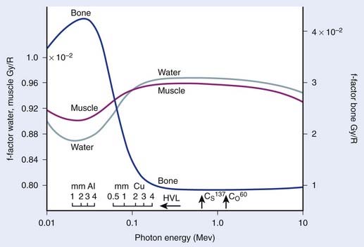
FIGURE 7-17 • The ratio of exposure to dose for bone, muscle, and water as a function of photon energy.
(From Johns HE, Cunningham JR: The physics of radiology, ed 4, Springfield, IL, 1983, Charles C. Thomas.)
Dose Determination Using Bragg-Gray Cavity Theory
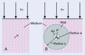
As mentioned, the exposure-based calibration method cannot be used above 3 MeV photon energies, so another technique must be used to evaluate dose at higher energies. The Bragg-Gray cavity theory is designed to directly relate the charge measured in a small air cavity in a phantom to the dose that would be delivered to the same point in the phantom in the absence of the air cavity. Fig. 7-18 shows a schematic drawing of the geometry of such a measurement. The Bragg-Gray theory2 states that if the air cavity is so small that it does not interfere with either the photons or their associated secondary electrons (an assumption that cannot be exactly true unless no ionizations are produced in the cavity) and if the cavity is located in a place where electronic equilibrium has been established, then
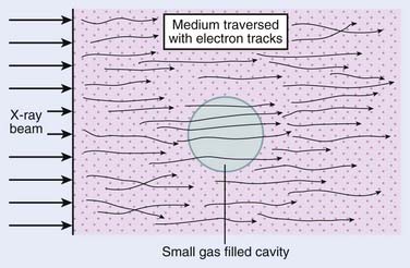
FIGURE 7-18 • Schematic drawing of a Bragg-Gray cavity in a medium exposed to an x-ray beam.
(From Johns HE, Cunningham JR: The physics of radiology, ed 4, Springfield, IL, 1983, Charles C. Thomas.)
where
that is, the product of the last two bracketed factors in Equation 2 is just the dose absorbed by the air in the cavity due to the interactions of the secondary electrons with the air. Note that because the cavity is very small, it is assumed that there are no direct interactions of the passing photons with the air molecules in the cavity, only the secondary electrons.
If we now replace the theoretical small air cavity with a realistic thimble ionization chamber as shown in Fig. 7-19, then we must assume that the chamber has a finite wall thickness of a material that may be different than the medium of the phantom. In this case, we have to modify the previous formula to account for electrons that are produced in the wall as well as in the phantom material and for a possible difference in the attenuation of the photons in the wall material versus the phantom. The Bragg-Gray theory, modified to account for this situation, leads to the following expression:
where
The first term in Equation 3 corresponds to electrons produced in the wall that interact in the air of the chamber and the second term to electrons that are produced in the medium. Obviously, if the wall is very thin, α is very close to zero and A is very close to 1.0, in which case Equation 3 becomes nearly identical to Equation 2.
Practical Dosimetry With Thimble Ionization Chambers
In 1983, the AAPM published a formalism for photon and electron dosimetry based on existing exposure or dose calibrations at 60Co energies.47 This formalism, called TG21, defines a parameter called Ngas = Dair/Mc (dose to the air of the chamber per unit meter reading in the calibration beam) that contains all the chamber-specific and calibration beam-specific parameters, including the 60Co exposure constant (Nx) or dose calibration constants. Knowledge of Ngas is equivalent to knowledge of the effective mass of air in the chamber. The quantity Ngas/Nx is a function of only the geometry of the chamber and the well-known properties of 60Co photons and is tabulated for specific thimble ionization chambers in the literature.47 This ratio can also be calculated from a knowledge of the materials and dimensions of the chamber. Once the Ngas for a chamber is known, the above formalism of Equation 3, based on Bragg-Gray cavity theory, can be used to obtain the dose to a medium for photons or electrons of arbitrary energy. That is, for photons of energy λ,
where
Similarly, for electrons of energy E
since one normally assumes that the electron beam will not be modified by the wall material, so the equation is simplified.
Dosimetry Based on Absorbed-Dose-to-Water Calibration
In 1999 the AAPM published the TG-51 dosimetry protocol for high-energy photons and electrons,48 which replaces TG-21 in most cases. In this protocol an absorbed-dose-to-water calibration factor for a 60Co beam,  , is determined for ionization chambers by a NIST-traceable calibration laboratory. Using the AAPM TG-51 protocol, the absorbed dose in the medium,
  , is related to the charge collected in the ionization chamber according to the formula
where M is the electrometer reading (i.e., the charge collected by the electrodes in the ion chamber) corrected for environmental temperature and pressure, ion recombination and polarity effects.  is the NIST-traceable absorbed-dose-to-water calibration factor for the ionization chamber in a 60Co beam. The factor, kQ, is a beam-quality conversion factor that is specified for different types of ionization chambers and adjusts
  for the quality, Q, of the beam in question. Quality conversion factors, kQ, have been tabulated for different types of ionization chambers and different photon beam energies (see Almond et al.48: Table I, p 1857). The value of kQ ranges from about 0.944 for a 24-MV photon beam to 1.0 for 60Co.
Thermoluminescent Dosimetry
In a crystal lattice, discrete electron energy levels are perturbed by the interactions between atoms, forming both allowed and forbidden energy bands. In the presence of certain impurities, energy traps can be formed in the forbidden region, and when irradiated, electrons can be excited out of their ground states into one of these forbidden energy traps. Since they are in the forbidden region, spontaneous decays back to the ground state are rare and the imprint of the absorbed dose remains until extra energy is provided to force the transition. This extra energy can be externally applied heat. By observing the heated TL material with a light-sensitive phototube, an electronic signal can be created that is proportional to the number of electrons in forbidden traps, which is, in turn, related to the energy absorbed by the TL material due to irradiation. Over a restricted range of absorbed dose, the response can be linear.59
The TL materials most commonly used for dosimetry are lithium fluoride, lithium borate, and calcium fluoride. They can be prepared in the form of powders, solid chips, and solid rods. By careful handling procedures, 3% to 5% reproducibility can be achieved after individual calibration of dosimeters with a photon beam.1,59 Because of their small size (typically <1 mm3 in volume) they are very conveniently used to attach to patient surfaces or place in patient cavities as in vivo dosimeters to verify dose calculations.
Solid State Detectors
Silicon diodes and other semiconductors can also be used to produce signals that are proportional to radiation dose. In a typical diode, there is a “p” region having an excess of positively charged “holes” and a depletion layer, or “n” region that has an excess of electrons. Radiation to the depletion layer produces electron-hole pairs that can cause current to flow across the junction between the layers if the diode has a reverse bias across it. The amount of current flow is proportional to the energy deposited by charged particles passing through the depletion layer.54 Silicon diodes have the great advantage of small size and a low-energy threshold for producing an ion pair, resulting in a high sensitivity. The disadvantage of the diode is that radiation damage causes a decrease in sensitivity with radiation dose.
Another solid state detector is the so-called “MOSFET,” an acronym for metal oxide semiconductor field effect transistor. A MOSFET detector for radiation dosimetry consists of two MOSFETs operating at different voltages. The difference in the threshold voltage shifts of the two MOSFETs is proportional to absorbed dose. Like diodes, these detectors are very small and sensitive and are now being used clinically at some institutions to evaluate dose in a phantom for highly complex dose distributions.60 They have been shown to be very linear over the range of doses of interest for radiotherapy verification. However, they have an angular dependence to radiation sensitivity that can limit their accuracy in clinical situations.
Film Dosimetry
Radiographic Film
where Io is the amount of light transmitted through an unexposed portion of the film and It is the amount of light transmitted through the exposed portion of interest. By carefully exposing and developing film to a series of known doses using the same photon energies as will be used for the test exposure, it is possible to obtain curves of optical density versus dose for specific emulsions from which absolute dose information can be subsequently extracted with some substantial uncertainty. This uncertainty is due to the fact that the silver in the emulsions strongly absorbs radiation below about 150 keV by the photoelectric process. For electrons, the information is much more trustworthy.
Radiochromic Film
Radiochromic film consists of thin layers (of the order of several to about 20 microns) of colorless radiosensitive dye sandwiched between a clear plastic material (e.g., Mylar or polyester). Unexposed film is a light blue-gray in color. After the film is exposed it darkens to a deep blue as a result of a polymerization process induced by ionizing radiation. The amount of darkening is related to the dose exposure of the film. Earlier forms of radiochromic film required high doses of radiation to achieve measurable film darkening. For example, GAFCHROMIC HD-810 film (International Specialty Products [ISP], Wayne, NJ) has been used in the dose range of 50 to 2500 Gy, and GAFCHROMIC MD-55 film (ISP, Wayne, NJ or Nuclear Associates, Carle Place, NY) is useful in the range of about 3 to 100 Gy. In 2004, a new form of radiochromic film, GAFCHROMIC EBT dosimetry film (ISP, Wayne, NJ) was introduced specifically for radiotherapy quality assurance (QA), in particular for intensity-modulated-radiotherapy (IMRT) fields. Several scientific papers have been published on the use of EBT film,61,62 and a white paper describing the product in detail can be found on the ISP website (http://www.ispcorp.com). GAFCHROMIC EBT film is ten times more sensitive than previous generation radiochromic films, with a dose range sensitivity of about 1 to 800 cGy. This implies that QA films can be irradiated in significantly less time, rendering QA procedures more efficient. Furthermore, all forms of radiochromic film exhibit significantly less energy dependence than radiographic film, primarily because radiochromic film is made with essentially water-equivalent materials (i.e., these films contain no high-Z elements such as silver).
Dose Distribution in Media
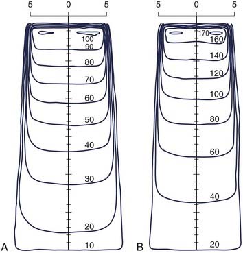
Percentage Depth Dose
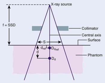
where Dd and Dref are dose rates at depth d below the surface and at the reference depth. This definition is described schematically in Fig. 7-20. In general, P depends on the depths d and ref, on the distance (f) from the source to the surface (often referred to as SSD), the field size on the surface (r), and the beam energy (E). The definition assumes that the field is square, so corrections must be made if rectangular or irregular field shapes are used.
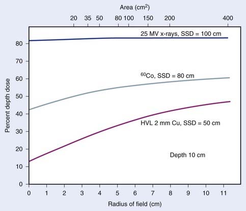
Percentage depth dose also increases with increasing field size due to the increasing contribution, with field size, of scatter to the dose on the central axis. As the field size is increased from zero, where we have only primary radiation, to a finite field size of radius r, the dose at all depths will increase due to the contribution of scatter. At deeper depths, where the field size is larger, the increase in dose will be larger than for shallower depths. For low energies and for small field sizes, the rate of change of the percent depth dose with field size will be fairly rapid. This variation of percent depth dose with field size for various energies is displayed in Fig. 7-21.
Compilations of central axis depth dose for various energies have been published63,64 and are summarized, for a few energies, in Fig. 7-22 for a fixed-field size of 10 cm × 10 cm. Of interest in this figure is the buildup of dose from the surface to a maximum value at a depth of dmax for high energy photons, and an increasing percentage depth dose with energy, for a fixed depth. The so-called buildup region near the surface for high-energy photon beams is due to the increase of secondary electron fluence with depth from the surface to a depth that corresponds approximately to the maximum range of the secondary electrons produced by the photons in the material of the phantom. The photon fluence, on the other hand, is exponentially decreasing with depth starting from the surface itself. The combination of these two effects yields a dose that is low at the surface, builds up to a maximum value at a depth that increases with the energy of the beam (and the maximum range of the secondary electrons), and then falls exponentially with depth beyond dmax. The rate of the exponential falloff in dose with depth beyond dmax is determined by the mean attenuation coefficient µ such that
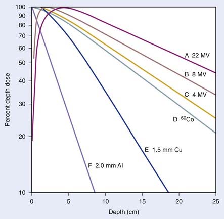
FIGURE 7-22 • Plot showing variation of dose with depth for 6 different energy photon beams.
(From Johns HE, Cunningham JR: The physics of radiology, ed 4, Springfield, IL, 1983, Charles C. Thomas.)
where Ks is the contribution of scatter to the dose on the central axis at depth d. It should be noted that the exact value of the dose in the buildup region and the depth of dmax are critically dependent on the design of the treatment head of the machine and the field size. The addition of any material near the surface of the patient or phantom, such as special blocks, produces electrons and thereby increases the surface dose65 and potentially changes the depth of maximal dose. For low-energy photons the buildup region is vanishingly small because of the combined effects of backscatter in the phantom and the short ranges of the secondary electrons produced in the phantom.
Correction of the PDD for rectangular fields (or irregular fields) requires that the integrated scatter from all points along the periphery of the field be calculated. The “equivalent square” field is that field, of radius r, that has the same integrated scatter as the field of interest. For rectangular fields, the equivalent square field must be found using published tables63 or by using the approximation
where S is the side of the equivalent square and L and W are the sides of the rectangle.
Tissue-Air Ratio
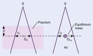
The use of PDD depends on SSD, as discussed earlier. This makes its use rather cumbersome, since in practical circumstances, the SSD may vary substantially across the field and from field to field. The tissue-air ratio (TAR) was introduced to allow dosimetry for rotational therapy, where the gantry moves around a fixed point in the patient.66 The TAR is defined as
where Dd is the dose rate at depth d in a phantom for field size rd defined at that depth, and Dfs is the dose rate in free space at the same point. The TAR concept is schematically represented in Fig. 7-23. The Dfs is measured with a small equilibrium mass around the point of interest to provide dose buildup. Since the point in the phantom and in free space are at the same distance from the source, TAR depends only on scatter and attenuation in the phantom. To the extent that phantom scatter is nearly independent of divergence of the beam, TAR is usually considered to be independent of SSD, an assumption that has been shown correct to within about 2% over the range of SSDs used clinically.67
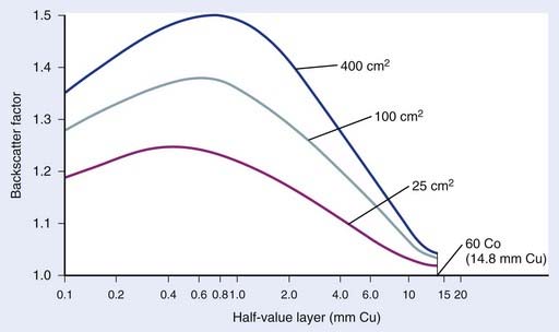
The TAR at dmax is given the special name backscatter factor (BSF), since the variation of this TAR from unity is a measure of the importance of scatter dose at dmax. As might be expected, BSF increases with increasing field size and decreases with increasing energy. The variation of BSF with HVL and field size is shown in Fig. 7-24. Above about 8 MV, the scatter contribution to the dose at dmax for all field sizes becomes negligibly small and BSF approaches unity.
Scatter-Air Ratio
The scatter-air ratio (SAR) is that portion of the TAR that is due to scatter. That is,

where TAR(d, 0, E) is the TAR for zero field size and represents the primary component of the TAR. The SAR concept is useful in calculating the net scatter dose to a point inside an irregular field.68 In this method, referred to as Clarkson’s method,69 radii are drawn at regular angular intervals from a point of interest inside an irregular field to the periphery of the field. The (SAR)avg is then calculated as the average SAR for all the intersections of these radii with the field edge, using the appropriate circular field SARs for each radial distance. Finally, the average TAR for the point of interest can be calculated as
More information on this technique can be found in textbooks on medical physics.1,2
Tissue-Phantom Ratio and Tissue-Maximum Ratio
The concept of TAR was developed partially to overcome the difficulty created by the dependence of PDD on SSD. As we go to higher photon energies, we encounter a difficulty with TAR due to the requirement of measuring a dose in free space. At low energies, the free space dose can be measured with a small buildup cap placed around the ion chamber to provide electron equilibrium. At high energies, however, this buildup cap becomes very thick and the attenuation of the beam in the cap as well as the effect of different materials in the cap and the wall must be considered. To avoid these difficulties, the concepts of tissue-phantom ratio (TPR)70 and tissue-maximum ratio (TMR)71 were developed. For both concepts, the reference dose and the dose of interest are measured in the phantom, thus, overcoming the difficulty of measuring a dose in free space. Like TAR, however, TMR and TPR are considered to be independent of SSD. The definitions are given by
and
where Dd is the dose rate on the central axis of the beam at the depth d for field size fd and Dref is the dose rate at the reference depth for the same field size. For the case of TMR this depth is dmax, whereas for TPR, the depth is some standard depth greater than dmax. One difficulty with TMR is created by the fact that the depth of dmax is a function of field size and SSD, thereby presenting a measurement problem.
where SAD is the source-to-isocenter distance, and [SAD + (d – diso)] is the source-to-calculation-point distance.
where  is the ratio of the phantom scatter at the reference depth for the field size fd to that for zero field size and where the reference depth is either dmax or dref for SMR or SPR. The phantom scatter factor ratio can be considered the same as the ratio of backscatter factors.
Dose Distributions
An isodose curve connects points of equal dose in a single plane. Frequently, one of the axes of the isodose curve display is the central axis of the beam, in which case the curves represent the variation in dose as a function of depth and transverse distance from the central axis. Fig. 7-25 shows two such displays for a 4-MV x-ray beam, one normalized to the maximum dose, and the other to the depth of the isocenter, that is the axis of rotation for an isocentric therapy unit. The shape of the isodose curves is affected by the beam parameters such as SSD, field size, and beam filter characteristics, as well as the shape of the entrance surface. Such curves are normally reconstructed after measuring at a large number of fixed points in a water phantom with an ionization chamber or diode. Computer-driven scanning probes are commercially available to help with this task.
Compensators and Wedge Filters
The most common form of compensator is the wedge filter. These wedges are normally constructed of brass, steel, or lead. When placed in the beam, they cause the isodose curves to be angled relative to the central axis. The wedge angle is defined as the angle between the isodose curve and a perpendicular to the central axis at some reference depth, often 10 cm. Wedges are normally furnished with commercial linear accelerators to produce wedge angles of 15, 30, 45, and 60 degrees. Examples of wedge isodose curves are shown in Fig. 7-26. When a wedge is used, a wedge factor must be defined, that is, the ratio of the dose rate at dmax on the central axis with the wedge in place to that with the wedge removed.
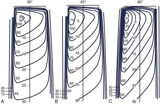
FIGURE 7-26 • Wedged isodose curves for 30-, 45-, and 60-degree wedges for a 10 cm × 10 cm field size.
(From Abrath FG, Purdy JA: Wedge design and dosimetry for 25-MV x-rays, Radiology 136:757, 1980.)
Patient-specific compensators are sometimes made to compensate for rapid variations in the patient surface over the field,72 although wedge filters are more commonly used for this purpose. Patient-specific compensators can be made of cells of high density metal distributed so as to attenuate the beam where the patient surface is far from the source, relative to those areas where the patient surface is closer.
Dose Calculations
Before the late 1980s, photon dose calculations were based primarily on interpolations of measured depth-dose data. Since these data are measured in homogeneous water phantoms for standard field sizes, corrections have to be made to account for tissue heterogeneities, sloping patient surfaces, and irregular field shapes. Mackie et al.73 has characterized this type of dose calculation as “correction-based.” Cunningham74 has described several commonly used tissue heterogeneity correction algorithms.
Advances in imaging and computing technologies have made it possible to incorporate sophisticated model-based dose calculation algorithms in clinical treatment planning systems. In model-based dose calculations, the treatment parameters, including the setup and patient geometry, are simulated from first principles by taking into account the physics of radiation transport. Measured relative dose quantities (e.g., percent depth dose and tissue phantom ratios) are used to verify the results of the model-based dose calculations, but they are not used directly to perform the calculation. Salient aspects of model-based photon dose calculation algorithms can be found in the review article of Ahnesjö and Aspradakis.75
Dose Calculations Based on Correction Methods

where
(the inverse square factor),
Further information on this can be found in the standard textbooks on medical physics.1,2
Correction for Non-Normal Beam Incidence
Effective Source-to-Skin Method
Fig. 7-27 illustrates the effective SSD method of correcting for surface obliquity. In this figure, S represents the patient surface, which is at a distance F from the source on the central axis, at a distance F + h′ above point p′ and a distance F − h′′ above point p′′. In this case, the dose on the central axis, Dc, gets modified at p′ and p′′ due to the decrease or increase in the overlying tissue relative to the central axis. However, an inverse square correction must be made because the points of interest are still at a distance of F + d from the source. The complete correction is
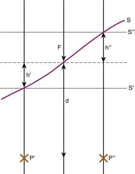
FIGURE 7-27 • Demonstration of the missing tissue method of calculating the effect of surface obliquity.
(From Williams JR, Thwaites DI: Radiotherapy physics in practice, Oxford, 1993, Oxford University Press.)
and
Corrections for Tissue Heterogeneities
The presence of tissues with electron densities different than water leads to a further modification of dose to points in the irradiated medium. The primary component of dose to any point is modified by any change in attenuation properties of overlying tissues. In addition, the scatter component of the dose will be influenced by the presence of neighboring inhomogeneities. This latter effect will be reduced for greater distances from the heterogeneities and for higher energies. There are a number of ways of correcting for the presence of tissue heterogeneities from very simple and fast approximations to more complex three-dimensional methods that are more accurate but much more computation-intensive. We discuss a few of these methods and refer the interested reader to other sources for more detailed information.1,3,76
Effective Depth Method
The simplest method of correcting for tissue heterogeneities involves simply calculating an effective depth, deff, for the point of interest, which is defined as the depth in unit density material that would result in the same net attenuation as the depth d in the phantom. Referring to Fig. 7-28, the effective depth of point p would be
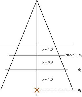
where PDD is the percent depth dose, and F is the source-to-surface distance. This method does not take account of the proximity of the inhomogeneity to the point of interest but is sufficiently accurate for many applications and simple enough to be calculated manually.
Tissue-Air Method

where Dp,uniform is the dose that would be measured at a true depth of d in a uniform phantom of water-equivalent material. This method considers both the beam size and the depth of the point of calculation and is probably more accurate than the effective depth method.
Equivalent Tissue-Air (ETAR) Method
A further improvement to the tissue-air method can be accomplished by using an effective field size as well as an effective depth.77 In this case,
where reff is the radius of a circular field that, when incident on unit density material, produces the same scatter dose to the point of interest as is observed for the inhomogeneous medium. For a uniform phantom of non–unit density material, the value of reff has been shown to scale directly with the density of the medium.78
Power Law Tissue-Air Ratio Method
In this method, the thickness and composition of overlying inhomogeneities are accounted for as well as the position of the calculation point relative to the inhomogeneity,79,80 although the lateral extent and shape of the inhomogeneity are not. Under the assumption that the calculation point is not very close to a boundary between two tissues of varying composition, the dose at point P in Fig. 7-28 can be written as

for the general case where the point of interest is imbedded in the nth layer of tissues,
where ρi is the density of the ith layer.
Other Methods of Correcting for Tissue Heterogeneities
The specific methods discussed to this point have been relatively simple approximations of the effect of tissue heterogeneities on the dose at an arbitrary point in a phantom. The most exact method would need to account for all scatter contributions to the dose at the point of interest. In principle, this can most be accomplished most accurately with a Monte Carlo calculation. This method uses the known cross sections for electron and photon interactions in matter and follows individual photons and their associated electrons through the entire phantom. By calculating the trajectories and interactions of a very large number of photon and electrons, one can accurately model the dose to all points within the heterogeneous phantom or patient. Recently, several Monte Carlo codes have been developed for radiotherapy treatment planning. These are discussed by a number of authors.81–90 Even with today’s fast computers such calculations are time consuming and not practical to use routinely. Monte Carlo is, however, a useful tool in testing the accuracy of simpler dose calculation methods as well as in providing input for the convolution/superposition methods discussed below.
Computed tomography is now routinely used as a basis for treatment planning. It provides the basis for target and normal tissue identification and location as well as a three-dimensional array of computed tomography numbers that are directly related to the electron density of the tissues. This array of electron densities can be used to calculate, the dose at each point, corrected for scatter from all other points in the phantom. It has been shown that such an approach yields only a marginal improvement in accuracy relative to the simpler tissue heterogeneity correction methods, described earlier.91
Model-Based Dose Calculations
At present, model-based dose calculation methods can be divided into two categories, those that use convolution/superposition principles to calculate dose73,92,93 and those that rely purely on Monte Carlo methods. Principles of the Monte Carlo method have been already been briefly described. Convolution/superposition calculations are defined by the basic equation
where
 ,
, is the point-spread function (also called the energy deposition kernel).
The point-spread function represents the fraction of the energy deposited (per unit volume) at some point ( ) in the calculation volume that is subsequently transported to the calculation point (
 ). The dose at any given point is, thus, computed by adding together (i.e., integrating over all space) the contributions from photons and electrons produced at all other points in the phantom or patient. Ahnesjö et al.94 found that the point-spread function changes only slightly as a function of energy (due to beam hardening), and that
  in the convolution integral from earlier, can be replaced by
  , the average dose-spread function weighted by the spectral components of the beam. Dose-spread functions for mono-energetic photons are generally precomputed using Monte Carlo methods.94 The energy dependence of the terma, TE, can be expressed by applying the inverse-square law and exponential attenuation to the photon fluence at the surface of the phantom or patient.
 , at each point within the phantom or patient and convolve the result with the point-spread function,
  . Essentially, the first part of the calculation takes into account the properties of the accelerator (including any beam-modifying devices used for the treatment), and the second part of the calculation takes into account the patient anatomy.
The convolution equation given earlier is strictly valid only for homogeneous media (i.e., the point-spread function must be spatially invariant). One way to model the effects of tissue heterogeneities is to replace all physical distances in the convolution integral with effective pathlengths. Many investigators have used this approximation.93–95 Details of this and other approximations that allow the convolution/superposition integral to be evaluated efficiently under many different conditions are not discussed here, but an excellent review is found in Webb’s book.96
The convolution/superposition algorithm can account for the effects of non–unit density material anywhere in the vicinity of the calculation point because it requires a three-dimensional integral over the entire radiation field. By contrast, most correction-based dose-calculation techniques require only a simple one-dimensional evaluation of effective pathlength, and can thus account for the effects of only those tissue heterogeneities that lie along a ray connecting the radiation source to the calculation point. Ahnesjö97 has tested the convolution method against Monte Carlo–generated data for simple layered as well as more complicated phantom geometries and found that the convolution model predicted the buildup dose and penumbra in the low-density regions fairly accurately. Lydon98 has tested the convolution model for clinical beams in homogeneous media and also obtained generally good results.
Monitor Unit Calculations
Fixed Source-to-Skin Distance Technique
where
Isocentric (Source-to-Isocenter) Technique
where
Monitor Unit Calculations for Convolution/Superposition Dose Calculations
where DQ is the dose at the dose-specification point Q (usually isocenter). The calibration factor, CF, is the measured dose per MU at the reference point for the calibration field. For convolution/superposition calculations, this reference point is typically selected to be sufficiently large (e.g., 10 cm) such that the effects of electron and photon contamination from the treatment head are negligible. ND is the normalized dose, defined as the dose per unit energy fluence at point Q relative to the dose per unit energy fluence at the reference point for the calibration field (i.e., the point at which CF is measured). fmod is the tray transmission factor, and OFC is the collimator output factor. OAR is the off-axis factor, which is required if the calculation point is not on the central axis.
OFC is determined from the relationship between phantom scatter and collimator scatter proposed by Khan1; that is, OFC = Sc,p/Sp, where Sc,p is the total scatter factor, and Sp is the phantom scatter factor. The total scatter factor is easily measured and is the ratio of the dose per MU in a phantom at the reference point for field size r to that measured at the reference depth for the standard field size (typically 10 cm × 10 cm). The phantom scatter factor, Sp, represents the ratio of the dose contributed from scattered radiation for a given field size at the reference point to that for a standard field size. This quantity is calculated directly for each clinical treatment field using the convolution/superposition model. The factor OFC is then obtained by dividing the measured Sc,p value by the calculated Sp value.

1 Khan FM. The physics of radiation therapy, ed 3. Philadelphia: Lippincott Williams and Wilkins; 2003.
2 Johns HE, Cunningham JR. The physics of radiology, ed 4. Springfield, Ill: Charles C Thomas; 1983. p 796
3 Williams JR, Thwaites DI. Radiotherapy physics in practice. Oxford: Oxford University Press; 1993. p 280
4 Hendee WR. Radiation therapy physics, ed 2. Chicago: Yearbook Medical Publishers; 1979. p 517
5 Amaldi U. Cancer therapy with particle accelerators. Nuclear Physics. 1999;A:375c.
6 Austin-Seymour M, Munzehrider JE, Goitein M, et al. Progress in low-LET heavy particle therapy: Intracranial and paracranial tumors and uveal melanomas. Radiat Res. 1985;104:S219.
7 Miller D. A review of proton beam radiation therapy. Med Phys. 22(Part 2), 1995.
8 Slater JM, Miller DW, Archambeau JO. Development of a hospital-based proton beam treatment center. Int J Radiat Oncol Biol Phys. 1988;14:761.
9 Castro JR, Chen GTY, Blakeley EA. Current considerations in heavy charged-particle radiotherapy: A clinical research trial of the University of California Lawrence Berkeley Laboratory, Northern California Oncology Group and Radiation Therapy Oncology Group. Radiat Res. 1985;104:S263.
10 Castro J, Phillips T, Prados M, et al. Neon heavy charged particle radiotherapy of glioblastoma of the brain. Int J Radiat Oncol Biol Phys. 1997;38:257.
11 Futami Y, Kanai T, Fujita M, et al. Broad-beam three-dimensional irradiation system for heavy-ion radiotherapy at HIMAC. Nuclear Instr Meth Physics Res. 1999;A:143.
12 Kraft G, Arndt U, Becher W, et al. Heavy ion therapy at GSI. Nuclear Instr Meth Physics Res. 1995;A:66.
13 Raju MR. Heavy particle radiotherapy. New York: Academic Press; 1980. p 500
14 Suzuki M, Kase Y, Yamaguchi H, Kanai T, Ando K. Relative bological effectiveness for cell-killing effect on various human cell lines irradiated with heavy-ion medical accelerator in Chiba (HIMAC) carbon-ion beams. Int J Radiat Oncol Biol Phys. 2000;48:241.
15 Orecchia R, Zurlo A, Loasses M, et al. Particle beam therapy (hadrontherapy): Basis for interest and clinical experience. Eur J Cancer. 1998;34:459.
16 Verhey L, Koehler A, McDonald J, et al. The determination of absorbed dose in a proton beam for purposes of charged-paraticle radiation therapy. Radiat Res. 1979;79:34.
17 Kanai T, et al. Biophysical characteristics of himac clinical irradiation system for heavy-ion radiation therapy. Int J Radiat Oncol Biol Phys. 1999;44:201.
18 Kraft G. Tumortherapy with ion beams. Nuclear Instr Meth Physics Res. 2000;A:1.
19 Douglas J, Laramore G, Austin-Seymour M, et al. Neutron radiotherapy for adenoid cystic carcinoma of minor salivary glands. Int J Radiat Oncol Biol Phys. 1996;36:87.
20 Douglas J, Laramore G, Autin-Seymour M, et al. Treatment of locally advanced adenoid cystic carcinoma of the head and neck with neutron radiotherapy. Int J Radiat Oncol Biol Phys. 2000;46:551.
21 Huber P, Debus J, Latz D, et al. Radiotherapy for advanced adenoid cystic carcinoma: Neutrons, photons or mixed beam? Radiother Oncol. 2001;59:161.
22 Raymond J, Vuong M, Russell K. Neutron beam radiotherapy for recurrent prostate cancer following radical prostatectomy. Int J Radiat Oncol Biol Phys. 1998;41:93.
23 Schwartz D, Einck J, Bellon J, et al. Fast neutron radiotherapy for soft tissue and cartilaginous sarcomas at high risk for local recurrence. Int J Radiat Oncol Biol Phys. 2001;50:449.
24 Bittner N, Koh WJ, Laramore G, et al. Treatment of locally advanced adenoid cystic carcinoma of the trachea with neutron radiotherapy. Int J Radiat Oncol Biol Phys. 2008.
25 Sauerwein W, Zurlo A. The EORTC Boron Neutron Capture Therapy (BNCT) Group: Achievements and future projects. Eur J Cancer. 2002;38:S31.
26 Yamamoto T, Matsumura A, Nakai K, et al. Current Clinical Results of the Tsukuba BNCT Trial. Appl Radiat Isot. 2004;61:1089.
27 Harling O, Riley K, Binns P, et al. The MIT user center for neutron capture therapy research. Radiat Res. 2005;165:221.
28 Henriksson R, Capala J, Michanek A, et al. Boron neutron capture therapy (BNCT) for globlastoma multiforme: A phase II study evaluating a prolonged high dose of boronophenylalanine (BPA). Radiother Oncol. 2008;88:183.
29 Yamamoto T, Nakai K, Matsumura A. Boron neutron capture therapy for glioblastoma. Cancer Letters. 2008;262:143.
30 Kankaanranta L, Seppälä T, Koivunoro H, et al. Boron Neutron Capture Therapy in the treatment of locally recurred head and neck cancer. Int J Radiat Onc Biol Phys. 2007;69:475.
31 Scalliet P, Remouchamps F, Lhoas M, et al. A retrospective analysis of the results of p(65) + Be neutrontherapy for the treatment of prostate adenocarcinoma at the Cyclotron of Louvain-la-Neuve. Part 1: Survival and progression-free survival. Cancer Radiother. 2001;5:262.
32 Palmer M, Goorley T, Kiger W, et al. Treatment planning and dosimetry for the Harvard-Mit phase I clinical trial of cranial neutron capture therapy. Int J Radiat Oncol Biol Phys. 2002;53:1361.
33 Allt WE. Supervoltage radiation treatment in advanced cancer of the uterine cervix: A preliminary report. J Can Med Assoc. 1969;100:792.
34 Johns HE, Bates LM, Watson TA. 1,000 Curie cobalt units for radiation therapy. 1. The Saskatchewan cobalt 60 unit. Br J Radiol. 1952;25:296.
35 Green DT, Errington RF. Design of a cobalt 60 beam therapy unit. Brit J Radiol. 1952;25:309.
36 Kerst DW. The betatron. Radiology. 1943;40:115.
37 Miller CW. Travelling-wave linear accelerator for x-ray therapy. Nature. 1953;171:297.
38 Purdy JA, Goer DA. Dual energy x-ray beam accelerators in radiation therapy: An overview. Nucl Inst Methods Phys Res. 1985;10/11:1090.
39 Karzmark CJ, Pering NC. Electron linear accelerators for radiation therapy: History, principles and contemporary developments. Phys Med Biol. 1973;18:321.
40 Karzmark CJ, Morton RJ. A Primer on Theory and Operation of Linear Accelerators in Radiation Therapy. Rockville, Md: US Bureau of Radiological Health; 1981.
41 Adler J, Murphy MJ, Chang SD, et al. Image-guided robotic radiosurgery. Neurosurg. 1999;44:1299.
42 Mackie T, Balog J, Ruchalak K, et al. Tomotherapy. Semin Radiat Oncol. 1999;9:108.
43 Reistad D, Brahme A. The microtron, a new accelerator for radiation therapy. In: 3rd International Conference on Medical Physics. Gøtenberg, Sweden: Chalmers University of Technology; 1972.
44 Svensson H, Jonsson L, Larsson LG, et al. A 22 MeV mictrotron for radiation therapy. Acta Radiol Ther Phys Biol. 1977;16:145.
45 Jongen Y, Beeckman W, Cohilis P. The proton therapy system for MGH’s NPTC: Equipment description and progress report. Bull Cancer Radiother. 1996;82(Suppl):219s.
46 Pedroni E, Bohringer T, Coray A, et al. Initial experience of using an active beam delivery technique at PSI. Strahlenther Onkol. 1999;175(suppl 2):18.
47 AAPM. American Association of Physicists in Medicine, A protocol for the determination of absorbed dose from high-energy photon and electron beams. Med Phys. 1983;10:741.
48 Almond PR, Biggs PJ, Coursey BM, Saiful Huq M, Nath R, Rogers DWO. AAPM’s TG-51 protocol for clinical reference dosimetry of high energy photon and electron beams. Med Phys. 1999;26:1847.
49 Domen SR, Lamperti PJ. A heat-loss compensated calorimeter: Theory, design and performance. J Res NBS. 1974;78A:595.
50 Schulz RJ, Wuu CS, Weinhous MS. The direct determination of dose-to-water using a water calorimeter. Med Phys. 1987;14:790.
51 Domen SR. A sealed water calorimeter for measuring absorbed dose. NIST J Res. 1994;99:121.
52 Domen SR. Absorbed dose water calorimeter. Med Phys. 1980;7:157.
53 McDonald JC, Domen SR. A-150 plastic radiometric calorimetry for charged particles and other radiations. Nucl Instr Methods Phys Res. 1986;752:35.
54 Attix F. Introduction to radiological physics and radiation dosimetry. New York: John Wiley and Sons; 1986. p 607
55 Seuntjens J, Palmans H. Correction factors and performance of a 4° C sealed water calorimeter. Phys Med Biol. 1999;44:627.
56 Fricke H, Hart EJ. Chemical dosimetry. In: Attix FH, Roesch WC, editors. Radiation dosimetry. New York: Academic Press, 1966.
57 ICRU: Stopping Powers for Electron Beams with Energies Between 1 and 50 MeV. International Commission on Radiation Units and Measurements, 1984.
58 CRU: Average Energy Required to Produce an Ion Pair. International Commission on Radiation Units and Measurements, 1979.
59 Cameron JR, Suntharalingam N, Kenney GN. Thermoluminescent dosimetry. Madison, Wisc: University of Wisconsin Press; 1968.
60 Chuang C, Verhey L, Xia P. Investigation of the use of MOSFET for clinical IMRT dosimetric verification. Med Phys. 2002;29:1109.
61 van Battum LJ, Hoffmans D, Piersma H, Heukelom S. Accurate dosimetry with GafChromic™ EBT film of a 6 MV photon beam in water: What level is achievable? Med Phys. 2008;35:704.
62 Wilcox E, Daskalov G, Nedialkova L. Comparison of the Epson Expression 1680 flatbed and the Vidar VXR-16 Dosikmetry PRO™ film scanners for use in IMRT dosimetry using Gafchromic and radiographic film. Med Phys. 2007;34:41.
63 Cohen M, Jones DEA, Greene D. Central axis depth dose data for use in radiotherapy. Br J Radiol. 1972;11(suppl):1.
64 Health Physics Association. Depth dose tables for use in radiotherapy. Br J Radiol. 1961;10(suppl):1.
65 Velkley DE, Manson DJ, Purdy JA. Build-up region of megavoltage photon radiation sources. Med Phys. 1975;2:14.
66 Johns HE, Whitmore G, Watson T, et al. A system of dosimetry for rotation therapy with typical rotation distributions. J Can Assn Radiol. 1953;4:1.
67 Johns HE, Bruce WR, Reid WB. The dependence of depth dose on focal skin distance. Br J Radiol. 1958;31:254.
68 Cunningham JR. Scatter-air ratios. Phys Med Biol. 1972;17:42.
69 Clarkson JR. A note on depth doses in fields of irregular shape. Br J Radiol. 1941;14:265.
70 Karzmark CJ, Deubert A, Loevinger R. Tissue-phantom ratios—An aid to treatment planning. Br J Radiol. 1965;38:158.
71 Holt JG, Laughlin JS, Moroney JP. The extension of the concept of tissue-air ratios (TAR) to high energy x-ray beams. Radiology. 1970;96:437.
72 Ellis F, Hall EJ, Oliver R. A compensator for variations in tissue thickness for high energy beams. Br J Radiol. 1959;32:421.
73 Mackie T, Scrimger J, Battista J. A convolution method for calculating dose for 15-MV x rays. Med Phys. 1985;12:188.
74 Cunningham J, Tissue inhomogeneity corrections in photon-beam treatment planning, ed; Orton C, editor; Progress in medical radiation physics; 1982; Plenum, New York:45.
75 Ahnesjö A, Aspradakis M. Dose calculations for external photon beams in radiotherapy. Phys Med Biol. 1999;44:99.
76 Coffey CW, Hines HC. Inhomogeneity corrections in treatment planning of the thorax. Am Assoc Med Dosimetrists J. 1983;8:6.
77 Sontag MR, Cunningham JR. The equivalent tissue-air ratio method for making absorbed dose calculations in a heterogeneous medium. Radiology. 1978;129:787.
78 O’Connor JE. The variation of scattered x-rays with density in an irradiated body. Phys Med Biol. 1957;1:352.
79 Young MEJ, Gaylord JD. Experimental tests of corrections for tissue inhomogeneities in radiotherapy. Br J Radiol. 1970;43:349.
80 Batho HF. Lung corrections in cobalt 60 beam therapy. J Can Assoc Radiol. 1964;15:79.
81 Ma C-M, Faddegon B, Rogers DWO, et al. Accurate characterization of the Monte Carlo beams for radiotherapy. Med Phys. 1997;24:401.
82 Ma C-M, Mok E, Kapur A, et al. Clinical implementation of a Monte Carlo treatment planning system. Med Phys. 1999;26:2133.
83 Ma C-M, Li J, Pawlicki T, et al. A Monte Carlo dose calculation tool for radiotherapy treatment planning. Phys Med Biol. 2002;47:1671.
84 Hartmann-Siantar C, Walling R, Daly T, et al. Description and dosimetric verification of the PEREGRINE Monte Carlo dose calculation system for photon beams incident on a water phantom. Med Phys. 2001;28:1322.
85 Faddegon B, Blogh J, Mackerzie R, et al. Clinical considerations of Monte Carlo for electron radiotherapy treatment planning. Radiat Phys Chem. 1998;35:217.
86 DeMarco J, Solberg T, Smathers J. A CT-based Monte Carlo simulation tool for dosimetry planning and analysis. Med Phys. 1998;25:1.
87 Wang L, Chui C, Lovelock M. A patient-specific Monte Carlo dose-calculation method for photon and electron radiotherapy treatment planning dose calculations. Med Phys. 1998;25:867.
88 Sempau J, Wilderman S, Bielajew A. DPM, a fast, accurate Monte Carlo code optimized for photon and electron radiotherapy treatment planning dose calculations. Phys Med Biol. 2000;45:2263.
89 Kawrakow I, Fippel M, Friedrich K. 3D electron dose calculation using voxel based Monte Carlo algorithm. Med Phys. 1996;23:479.
90 Chetty I, Moran J, Nurusher T, et al. Experimental validation of the DPM Monte Carlo code using minimally scattered electron beams in heterogeneous media. Phys Med Biol. 2002;47:1837.
91 Parker RP, Hobday PA, Cassell KJ. The direct use of CT numbers in radiotherapy dosage calculations for inhomogeneous media. Phys Med Biol. 1979;24:802.
92 Boyer A, Mok E. A photon dose distribution model employing convolution calculations. Med Phys. 1985;12:169.
93 Mohan R, Chui C, Lidofsky L. Differential pencil beam dose computation model for photons. Med Phys. 1986;13:64.
94 Ahnesjö A, Andreo P, Brahme A. Calculation and application of point spread functions for treatment planning with high energy photon beams. Acta Oncol. 1987;26:49.
95 Nilsson M, Knöös T. Application of the Fano theorem in inhomogeneous media using a convolution algorithm. In: 1st Biennial ESTRO Meeting on Physics in Clinical Radiotherapy. Budapest: European Society for Therapeutic Radiology and Oncology; 1991.
96 Webb S. The physics of three-dimensional radiation therapy. Medical Science Series. Bristol and Philadelphia: IOP Publishing, Ltd; 1993. p 373
97 Ahnesjö A. Collapsed cone convolution of radiant energy for photon dose calculation in heterogeneous media. Med Phys. 1989;16:577.
98 Lydon J. Photon dose calculations in homogeneous media for a treatment planning system using a collapsed cone superposition convolution algorithm. Phys Med Biol. 1998;43:1813.
[/level-membership-for-hematology-oncology-and-palliative-medicine-category][not-level-membership-for-hematology-oncology-and-palliative-medicine-category]
7 Principles of Radiation Physics
In this chapter, we present the basic radiation physics needed for the practice of radiation oncology. Many of the specific applications of these basic physics principles, such as brachytherapy and treatment planning, are presented elsewhere in this textbook. Since the primary audience for this textbook is assumed to be practicing radiation oncologists and resident clinicians, many topics are not treated in the detail that would be required by radiation physicists. Excellent physics textbooks that present the topics in more depth are available.1–4
Basic Concepts
Atomic and Nuclear Structure
In the planetary model of the atom, first described by Niels Bohr, the electron orbits make up discrete concentric shells, with a different binding energy associated with each shell. The shells are labeled K, L, M, and so on from the innermost to the outermost shell. The maximum number of electrons allowed in each shell is 2n2, where n = 1 for the K shell, n = 2 for the L shell, and so on. Therefore, there are up to 2 electrons in the K shell, 8 in the L shell, 18 in the M shell, and so on. A simple schematic drawing of the Bohr model is shown in Fig. 7-1.
Nuclear Transformations
The explanation of nuclear decay depends on understanding the interplay between the very strong, attractive nuclear force that binds the neutrons and protons together in the nucleus, and the moderately strong repulsive electromagnetic force between the protons. As the protons and neutrons move about within the nucleus, there is some probability that one of them will acquire enough kinetic energy to escape from the nuclear potential energy “well.” Large nuclei with many neutrons and protons tend to be less stable because of the increasing repulsion of the protons. For large nuclei to be stable, an excess of neutrons is required to provide the nuclear attraction to keep the protons from escaping. Fig. 7-2 shows the line of stable nuclei for the range of known elements.
FIGURE 7-2 • Plot of numbers of neutrons and protons in stable nuclei.
(From Khan FM: The physics of radiation therapy, ed 3, Philadelphia, 2003, Lippincott Williams & Wilkins, p 4.)
Decay Constant
where N is the number of radioactive nuclei and λ is the decay constant. The minus sign indicates that the number of nuclei is decreasing with time. Integration of this differential equation leads to the following equation:
where N0 is the number of radioactive nuclei initially present, N(t) represents the number remaining at time t, and e is the base of the natural logarithm (2.71828).
where A0 is the initial activity and A(t) is the activity at time t. The unit of activity is the Curie (Ci) or the Becquerel (Bq), which is 1 disintegration per second:
Half-Life and Mean Life
the mean or average life (Tλ) is the time for the number of atoms to decay to 1/e of the initial number, so
Radioactive Decay Series and Equilibrium
In each series, the half-life of the parent is longer than any of the half-lives of any of the daughter nuclides. This phenomenon leads to a state of transient or secular equilibrium. Since each daughter is less stable than the original parent, the activity of the daughter will increase with time, until it approaches the activity of the long-lived parent. If the half-lives are very different, the activities will become essentially identical after a number of daughter half-lives, and this is called secular equilibrium. An example is shown in Fig. 7-3. If the half-lives of the parent and daughter are very similar, transient equilibrium is reached in a few half-lives, after which the daughter has an activity in excess of the parent activity but decays with the same rate as the limiting parent decay rate. An example of this phenomenon is shown in Fig. 7-4. For either case, after a time that is long compared to the half-life of the shorter-lived nuclide,
FIGURE 7-3 • Example of secular equilibrium in the decay of 226Ra to 222Rn.
(From Khan FM: The physics of radiation therapy, ed 3, Philadelphia, 2003, Lippincott Williams & Wilkins, p 19.)
where Ai and Ti refer to the activity and half-life of the daughter (d) or parent (p).
X-Ray Production
Characteristic X-Rays
When electrons are incident on target atoms, they can ionize those atoms by depositing sufficient energy to eject an inner shell electron. The inner shell vacancy is subsequently filled by an outer shell electron, causing the emission of a characteristic x-ray with energy equal to the difference between the binding energies of the inner and outer shells. This process is diagrammed in Fig. 7-5. Although this process can take place in both low-Z and high-Z atoms, only for high-Z atoms are the binding energies sufficient to produce radiation in the x-ray portion of the electromagnetic spectrum. For example, the binding energy of K-shell electrons in tungsten, a common target for x-ray tubes and accelerators, is about 70 keV, whereas for aluminum, it is only about 1.5 keV. As mentioned earlier, the characteristic x-ray energy is occasionally transferred directly to an orbital electron, leading to the production of an Auger electron.
Bremsstrahlung X-Rays
In general, both bremsstrahlung and characteristic x-rays are present when electrons strike a target. Fig. 7-6 shows x-ray spectra for a thick tungsten target for electron energies of from 65 keV to 200 keV. Note the appearance of the characteristic x-rays on top of the bremsstrahlung spectrum once the electron energy is in excess of the K-shell binding energy of 70 keV. Any material in the x-ray beam, including the target itself, will absorb some of the energy of the beam. The effect of such absorption is to preferentially filter out the low energy portion of the bremsstrahlung spectrum. The process of preferentially attenuating the low-energy component of the beam is referred to as “beam hardening.” When the beam is hardened, the average energy of the x-rays increases at the expense of reduced intensity.
Interaction of X-Rays and Particles With Matter
X-Ray Interactions
where dN is the reduction in the number of photons due to interactions in a thickness dx of an absorber, N is the number of incident photons, and µi is the attenuation coefficient for the ith interaction process. After integration over the thickness, this equation becomes
where N(x) is the number of photons left in the beam (without interaction) as a function of the thickness x of material traversed, and µtot is the sum of the individual attenuation coefficients. (µi/ρ) is called the mass-attenuation coefficient for process i, where ρ is the density of the material. Dividing the conventional attenuation coefficients by density removes the dependence on the physical density of materials and the resulting mass attenuation coefficients are approximately equal from material to material. The corresponding thickness, ρx, is in units of grams per square centimeter (g/cm2). The total mass attenuation coefficients for water and lead are shown as functions of energy in Fig. 7-7. There are five different photon interaction processes, including coherent scattering, photoelectric effect, Compton scattering, pair production, and photodisintegration. These will be discussed in turn.
implying that
Compton Scattering
Compton scattering is a process in which the incident photon interacts with an orbital electron as if it were a free particle, since the binding energy is small compared to the photon energy. The dynamics of the interaction can be described as a typical particle–particle scattering interaction whereby the photon transfers some of its energy to the electron and is scattered at an angle φ relative to the incident direction. The electron is ejected at an angle θ relative to the forward direction. The energy of the outgoing Compton-scattered photon is equal to the difference between the incident photon energy and the energy transferred to the electron. A diagram of the Compton process is shown in Fig. 7-8.
FIGURE 7-8 • Illustration of the Compton effect.
(From Khan FM: The physics of radiation therapy, ed 3, Philadelphia, Lippincott Williams & Wilkins, p 67.)
From conservation of momentum:
and
where ve is the velocity of the electron, me is the rest mass of the electron, c is the speed of light, and
Solving these three simultaneous equations, we obtain the following relationships:
where α = hνo/ mec2 and f = (1 − cos φ).
Relative Importance of Interaction Types
The total mass absorption coefficient is the sum of the coefficients for coherent, photoelectric, Compton, and pair production. For low-Z targets such as tissue (average Z = 7), Compton processes are overwhelmingly dominant throughout the range of energies used in therapy. Fig. 7-9 shows the relative importance of photoelectric, Compton, and pair production as a function of photon energy and the atomic number of the target material.4 For tissue, Compton dominates between approximately 30 keV and 30 MeV, whereas for lead, photoelectric dominates up to approximately 800 keV and pair production above about 5 MeV. Because of its calcium content, bone has a higher absorption by photoelectric and pair production. This leads to high bone doses for orthovoltage and kilovoltage and for higher energy accelerator beams.
Charged Particles
Electrons
Electrons lose energy to the medium by two processes, ionization and radiation. Ionization processes are interactions with the atomic electrons, whereas radiation losses are interactions with the field of the nucleus, leading to bremsstrahlung x-ray production. Whereas the microscopic interactions are well understood, the macroscopic description of the energy and range of the particles at any point in the medium is not simple. This is because the electrons are very much lighter than the atomic nuclei. Therefore, the electron can lose a very large fraction of its energy in a single process and can be deflected by very large angles. This means that even if the electron beam is monoenergetic when entering a medium, there will be a large amount of range-straggling, or a large variation from electron to electron as to where, in the phantom, the electron will stop. Fig. 7-10 shows a plot of absorbed dose as a function of depth for monoenergetic electrons incident on water. There is a depth beyond which the dose is almost zero, where all the incident electrons have been stopped and where the remaining dose is due to bremsstrahlung x-rays produced by the electrons in the medium. This is in sharp contrast to the exponential falloff of dose for x-rays. This ranging out of electrons in matter is responsible for the popularity of electrons for treatment of superficial disease.
Protons and Heavier Ions
The use of protons and heavy ions for radiotherapy was pioneered in the 1970s and 1980s at the Massachusetts General Hospital in collaboration with the now decommissioned Harvard Cyclotron Laboratory and at the Lawrence Berkeley National Laboratory in Berkeley, California.5–15 Since then, several proton and charged-particle facilities have been built around the world, a list of which can be found on the website for the Particle Therapy Co-Operative Group (PTCOG; http://ptcog.web.psi.ch/). Similar to electrons, protons lose energy primarily by electromagnetic interactions with the atomic electrons. A major difference between protons and electrons is that protons are much heavier than electrons and therefore lose only a very small fraction of their energy in an individual interaction, scattering minimally in the process. Protons lose energy at an increasing rate as they slow down, yielding an enhanced region of energy deposition called the Bragg Peak just before they stop. One can predict very accurately the depth at which the protons will come to rest if the initial energy of the protons and the electron density of the material traversed are known. The absence of exit dose beyond the intended target makes protons nearly ideally suited for optimal physical dose delivery. A typical depth dose distribution for a clinical, energy-modulated proton beam, compared to that of a 10-MV bremsstrahlung x-ray beam, is shown in Fig. 7-11. A small percentage of proton interactions is via nuclear interactions with the nucleus. These rare interactions are qualitatively different than electromagnetic interactions and are thought to be responsible for enhancing the cell kill per unit dose by about 10% to 20% over that of x-rays.16
Heavy ions such as helium, carbon, neon, and argon nuclei have also been used in radiotherapy.9–12,14,15,17,18 Similar to protons, they lose energy by interacting with the atomic electrons. Being even heavier than protons, they scatter even less and have even more rapid dose falloff outside the central beam and even faster falloff of dose beyond the end of range. In addition to these electromagnetic interactions, heavy ions have a probability of interacting with the nucleus via nuclear interactions that increases with the mass of the incident ion. In particular, as the heavy ions begin to slow down, they tend to suffer nuclear interactions in which they lose a very large amount of their energy in a single event. This high density of deposited energy kills cells in a far more efficient way per unit dose than x-rays. These particles are said to have a high radiobiologic efficiency (RBE). For more information on these particles, the reader is referred to the literature.13
Neutrons
Neutrons have also been used in clinical treatments.19–24 These particles are neutral, so they cannot lose energy by any means other than the nuclear interaction. All of their interactions are “catastrophic,” because a significant portion of their energy is deposited in an individual event. Their primary interactions are with protons within the nucleus. These nuclear events result in recoil protons and charged nuclear fragments that have rather low energy and deposit large amounts of energy very close to the site of the original interaction. The falloff of neutron dose with depth is exponential and similar to that of low-energy x-rays, with the depth of the 50% dose being around 10 cm for typical treatment energies. Neutrons are very efficient in producing cell kill per unit dose (high RBE) relative to x-rays for both tumor tissue and normal tissues. Clinical trials have been conducted to investigate the areas where neutrons might have an advantage over x-rays. A summary of the physical characteristics and results of early clinical results is available.13
In addition, clinical trials are under way to investigate the use of slow neutrons, either thermal or epithermal in energy, to treat boronated tumor cells in patients.25–32 The clinical efficacy of these neutrons for cancer therapy depends on the very high cross section for neutron capture by boron and on a high ratio of boron in the tumor cells to that in the surrounding normal cells. To date, clinical results of these trials have been disappointing.
Radiation Therapy Treatment Machines
Kilovoltage Units
A schematic diagram of an x-ray tube suitable for radiation therapy is shown in Fig. 7-12. Since a high-voltage supply is used to generate the accelerating potential for the electron beams, a maximum energy of approximately 300 kV is achievable with this design. The resulting x-ray beams have a spectrum of photon energies with a maximum equal to the energy of the electron beam.
FIGURE 7-12 • Schematic diagram of an x-ray tube that could be used for radiation therapy.
(From Khan FM. The physics of radiation therapy, ed 3, Philadelphia, Lippincott Williams & Wilkins, p 29.)
Megavoltage Units
X-ray and γ-ray beams of energy greater than 1 MV are classified as megavoltage beams. In the 1930s a number of transformer-based and van de Graaff generator–based units working in the 800 KeV to 2 MeV range were installed around the world. However, it was not until the introduction of the 60Co teletherapy machine and the linear accelerator that the routine use of megavoltage x-ray and γ-ray beams occurred, significantly changing the practice of radiotherapy and leading to substantial improvements in clinical results.33
Teletherapy Machines
The megavoltage era began with the introduction of the 60Co teletherapy machine into radiotherapy clinics beginning in 1951.34,35 The development of nuclear reactors in the late 1940s made possible the production of small 60Co sources with specific activities (in Curies per gram) high enough to produce clinically acceptable dose rates of more than 1 Gray (Gy) per minute at a typical treatment distance of 80 cm from the source. These machines quickly became the standard of radiotherapy because of their simplicity of design and operation, low cost, and availability. The two photons produced by the decay of 60Co have energies of 1.17 and 1.33 MeV, yielding a depth-dose curve that falls to 50% of maximum in about 10 cm of water or tissue. In addition, the relatively high energy of the photons leads to “skin sparing” due to a reduced entrance dose that builds up for a distance of 5 mm (the maximum range of the secondary electrons from 60Co photons) to a maximum value. The half-life of 60Co is 5.27 years, making the source change a relatively infrequent requirement. With the highest specific activities currently achievable, dose rates of at least 1.5 Gy per minute for a field size of 40 cm × 40 cm can be achieved at 80 cm source-to-treatment distance.
Betatrons
The next chronological development in treatment machines is the betatron, first developed by D. W. Kerst at the University of Illinois36 primarily for physics experimentation. Electrons with energies of up to 45 MeV have been produced in betatrons for radiotherapy and used either directly or to produce bremsstrahlung x-ray beams. The massive size of these machines, their high cost, and relatively low dose rate combined to limit their usefulness in radiation therapy.
Linear Accelerators
The use of microwaves to accelerate electrons to high energies for radiotherapy was first demonstrated in Great Britain in 1953.37 This became possible primarily because of the development of high-power microwave generators for military radar use during World War II. The major components of a typical medical linear accelerator (linac) are shown in a block diagram in Fig. 7-13. The acceleration of the electron beam takes place in the accelerator wave guide, consisting of a stack of cylindrical cavities with a hole through the center, into which resonant electromagnetic waves of frequency in the microwave range (∼3000 MHz) have been coupled. The electron beam is created and preaccelerated to approximately 50 keV in a conventional electrostatic electron gun, injected into the resonating waveguide, spatially bunched and accelerated through interactions with the electromagnetic field in the individual cavities, and then emerges from the accelerating structure as a narrow pencil beam that can be magnetically bent or focused onto a scattering foil (for electron treatments) or a bremsstrahlung target (for x-ray treatments) in the treatment head of the linac. For low energies of 6 MeV or less, the beam can be magnetically focused in the forward (vertical) direction onto the axis of the treatment head, whereas at higher energies, the beam is usually bent through a 90-degree or 270-degree angle before entering the treatment head since the accelerating structure is much longer for high energies and is frequently oriented horizontally to save space. For more details about the acceleration process, the reader is referred to several excellent review articles in the literature.38–40
FIGURE 7-13 • A block diagram of a typical medical linear accelerator.
(From Khan FM: The physics of radiation therapy, ed 3, Philadelphia, 2003, Lippincott Williams & Wilkins, p 43.)
Although the details of the acceleration process can be quite technical, the shaping of the beam in the treatment head is both important and conceptually easy to understand. Fig. 7-14
[/not-level-membership-for-hematology-oncology-and-palliative-medicine-category]
