3 Practical pharmacokinetics
General applications
Time to maximal response
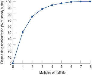
By knowing the half-life of a drug, the time to reach a steady state may be estimated (Fig. 3.1), and also when the maximal therapeutic response is likely to occur, irrespective of whether drug level monitoring is needed.
Application to therapeutic drug monitoring
Clinical pharmacokinetics is usually associated with therapeutic drug monitoring (TDM), and its subsequent utilisation. When TDM is used appropriately, it has been demonstrated that patients suffer fewer side effects than those who are not monitored (Reid et al., 1990). Although TDM is a proxy outcome measure, a study with aminoglycosides (Crist et al., 1987) demonstrated shorter hospital stays for patients where TDM was used. Furthermore, a study on the use of anticonvulsants (McFadyen et al., 1990) showed better epilepsy control in those patients where TDM was used. A literature review of the cost-effectiveness of TDM concluded that emphasis on just cost is inappropriate and clinical relevance should be sought (Touw et al., 2007). There are various levels of sophistication for the application of pharmacokinetics to TDM. Knowledge of the distribution time and an understanding of the concept of steady state can facilitate determination of appropriate sampling times.
Basic concepts
Volume of distribution

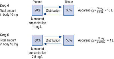
This relationship assumes that the drug is evenly distributed throughout the body in the same concentration as in the plasma. However, this is not the case in practice, since many drugs are present in different concentrations in various parts of the body. Thus, some drugs which concentrate in muscle tissue have a very large apparent volume of distribution, for example digoxin. This concept is better explained in Fig. 3.2.
Conversely, if the desired concentration is known, the loading dose may be determined:

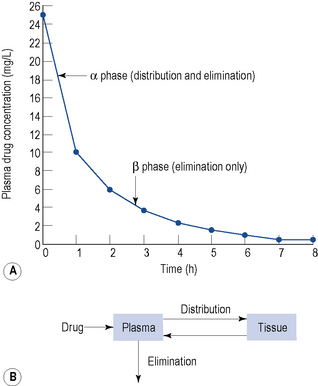
Figure 3.3 depicts the disposition of a drug immediately after administration and relates this to the plasma concentration–time graph.
Elimination


The clearance of most drugs remains constant for each individual. However, it may alter in cases of drug interactions, changing end-organ function or autoinduction. Therefore, it is clear from equation (Eq.) (3) that as the plasma concentration changes so will the rate of elimination. However, when the rate of administration is equal to the rate of elimination, the plasma concentration is constant (Css) and the drug is said to be at a steady state.

At the beginning of a dosage regimen the plasma concentration is low. Therefore, the rate of elimination from Eq. (3) is less than the rate of administration, and accumulation occurs until a steady state is reached (see Fig. 3.1).

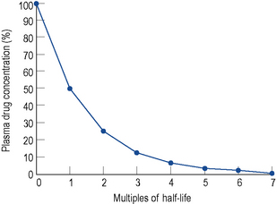
It is clear from Eq. (3) that as the plasma concentration falls (e.g. on stopping treatment or after a single dose), the rate of elimination also falls. Therefore, the plasma concentration–time graph follows a non-linear curve characteristic of this type of first-order elimination (Fig. 3.4). This is profoundly different from a constant rate of elimination irrespective of plasma concentration, which is typical of zero-order elimination.

Combining Eqs. (3) and (5) gives

and since

then
Elimination half-life (t1/2) is the time it takes for the plasma concentration to decay by half. In five half-lives the plasma concentration will fall to approximately zero (see Fig. 3.4).
The equation which is described in Fig. 3.4 is
where C1 and C2 are plasma concentrations and t is time.
If half-life is substituted for time in Eq. (7), C2 must be half of C1.
There are two ways of determining ke, either by estimating the half-life and applying Eq. (8) or by substituting two plasma concentrations in Eq. (7) and applying natural logarithms:


In the same way as it takes approximately five half-lives for the plasma concentration to decay to zero after a single dose, it takes approximately five half-lives for a drug to accumulate to the steady state on repeated dosing or during constant infusion (see Fig. 3.1).
This graph may be described by the equation
where C is the plasma concentration at time t after the start of the infusion and Css is the steady state plasma concentration. Thus (if the appropriate pharmacokinetic parameters are known), it is possible to estimate the plasma concentration any time after a single dose or the start of a dosage regimen.
Absorption
The rate of elimination of a drug after a single dose is given by Eq. (3). By definition the rate of elimination is amount of drug eliminated per unit time.
The amount eliminated in any one unit of time 

As previously explained, CL is constant. Therefore,

 from start until zero is actually the area under the plasma concentration–time curve (Fig. 3.5).
After a single i.v. dose the total amount eliminated is equal to the amount administered D i.v.
 or
or 
However, for an oral dose the amount administered is 
As CL is constant in the same individual,


In this way, F can be calculated from plasma concentration–time curves.
Dosing regimens
From Eq. (1) we can determine the change in plasma concentration ΔC immediately after a single dose:
where F is bioavailability and S is the salt factor, which is the fraction of active drug when the dose is administered as a salt (e.g. aminophylline is 80% theophylline, therefore S = 0.8).
Conversely, to determine a loading dose:
At the steady state it is possible to determine maintenance dose or steady state plasma concentrations from a modified Eq. (4):

where T is the dosing interval.
Peak and trough levels
Substituting Cssmax for C1 and Cssmin for C2 in Eq. (7):
where t is the dosing interval.
If this is substituted into the preceding equation:
Interpretation of drug concentration data
Sampling times
In the preceding sections, the time to reach the steady state has been discussed. When TDM is carried out as an aid to dose adjustment, the concentration should be at steady state. Therefore, approximately five half-lives should elapse after initiation or after changing a maintenance regimen, before sampling. The only exception to this rule is when toxicity is suspected. When the steady state has been reached, it is important to sample at the correct time. It is clear from the discussion above that this should be done when distribution is complete (see Fig. 3.3).
Dosage adjustment
Under most circumstances, provided the preceding criteria are observed, adjusting the dose of a drug is relatively simple, since a linear relationship exists between the dose and concentration if a drug follows first-order elimination (Fig. 3.6A). This is the case for most drugs.
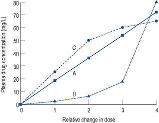
Capacity limited clearance
If a drug is eliminated by the liver, it is possible for the metabolic pathway to become saturated, since it is an enzymatic system. Initially the elimination is first-order, but once saturation of the system occurs, elimination becomes zero-order. This results in the characteristic dose–concentration graph seen in Fig. 3.6B. For the majority of drugs eliminated by the liver, this effect is not seen at normal therapeutic doses and only occurs at very high supratherapeutic levels, which is why the kinetics of some drugs in overdose is different from normal. However, one important exception is phenytoin, where saturation of the enzymatic pathway occurs at therapeutic doses. This will be dealt with in the section on phenytoin.
Increasing clearance
The only other situation where first-order elimination is not seen is where clearance increases as the plasma concentration increases (Fig. 3.6C). Under normal circumstances, the plasma protein binding sites available to a drug far outnumber the capacity of the drug to fill those binding sites, and the proportion of the total concentration of drug which is protein bound is constant. However, this situation is not seen in one or two instances (e.g. valproate and disopyramide). For these particular drugs, as the concentration increases the plasma protein binding sites become saturated and the ratio of unbound drug to bound drug increases. The elimination of these drugs increases disproportionate to the total concentration, since elimination is dependent on the unbound concentration.
Clinical applications
Estimation of creatinine clearance
Since many drugs are renally excreted, and the most practical marker of renal function is creatinine clearance, it is often necessary to estimate this in order to undertake dosage adjustment in renal impairment. The usual method is to undertake a 24-h urine collection coupled with a plasma creatinine measurement. The laboratory then estimates the patient’s creatinine clearance. The formula used to determine creatinine clearance is based upon the pharmacokinetic principles in Eq. (3).

Using this rate of excretion and substituting the measured plasma creatinine for Css in Eq. (4), the creatinine clearance can be calculated.
Therefore, equations have been produced which are rearrangements of Eq. (4), that is,
It has been shown that the equation produced by Cockcroft and Gault (1976) appears to be the most satisfactory. A modified version using SI units is shown as

where F = 1.04 (females) or 1.23 (males).
There are limitations using only plasma creatinine to estimate renal function. The modification of diet in renal disease (MDRD) formula can be used to estimate glomerular filtration rate (eGFR). This formula uses plasma creatinine, age, sex and ethnicity (Department of Health, 2006).
Digoxin
Distribution
Digoxin is widely distributed and extensively bound in varying degrees to tissues throughout the body. This results in a high apparent volume of distribution. Digoxin volume of distribution can be estimated using the equation 7.3 L/kg (ideal body weight (BWt)) which is derived from population data. However, distribution is altered in patients with renal impairment, and a more accurate estimate in these patients is given by:

A two-compartment model best describes digoxin disposition (see Fig. 3.3), with a distribution time of 6–8 h. Clinical effects are seen earlier after intravenous doses, since the myocardium has a high blood perfusion and affinity for digoxin. Sampling for TDM must be done no sooner than 6 h post-dose, otherwise an erroneous result will be obtained.
Theophylline
Elimination
Gentamicin
Practical implications
Initial dosage
This may be based on the patient’s physiological parameters. Gentamicin clearance may be determined directly from creatinine clearance. The volume of distribution may be determined from ideal body weight. The elimination constant ke may then be estimated using these parameters in Eq. (6). By substituting ke and the desired peak and trough levels into Eq. (7), the optimum dosage interval can be determined (add on 1 h to this value to account for sampling time). Using this value (or the nearest practical value) and the desired peak or trough value substituted into Eq. (13) or Eq. (14), it is possible to determine the appropriate dose.
Changing dosage
This is not as straightforward as for theophylline or digoxin, since increasing the dose will increase the peak and trough levels proportionately. If this is not desired, then use of pharmacokinetic equations is necessary. By substituting the measured peak and trough levels and the time between them into Eq. (7), it is possible to determine ke (and the half-life from Eq. (8) if required). To estimate the patient’s volume of distribution from actual blood level data, it is necessary to know the Cssmax immediately after the dose (time zero), not the 1 h value which is measured. To obtain this, Eq. (7) may be used, this time substituting the trough level for C2 and solving for C1. Subtracting the trough level from this Cssmax at time zero, the volume of distribution may be determined from Eq. (10). Using these values for ke and Vd, derived from actual blood level data, a new dose and dose interval can be determined as before.
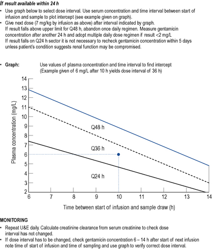
Once daily dosing
Initial dosage for a once daily regimen is 5–7 mg/kg/day for patients with a creatinine clearance of >60 mL/min. This is subsequently adjusted on the basis of blood levels. However, monitoring of once daily dosing of gentamicin is different to multiple dosing. One approach is to take a blood sample 6–14 h after the first dose and plot the time and result on a standard concentration-time plot (the Hartford nomogram, Nicolau et al., 1995; Fig. 3.7). The position of the individual patient’s point in relation to standard lines on the nomogram indicates what the most appropriate dose interval should be (either 24, 36 or 48 h). Once daily dosing of gentamicin has not been well studied in pregnant or breastfeeding women, patients with major burns, renal failure, endocarditis or cystic fibrosis. Therefore, it cannot be recommended in these groups and multiple daily dosing should be used.
Lithium
Distribution
Lithium is unevenly distributed throughout the body, with a volume of distribution of approximately 0.7 L/kg. Lithium follows a two-compartment model (see Fig. 3.3) with a distribution time of 8 h (hence, the 12-h sampling criterion).
Phenytoin
Phenytoin is used in the treatment of epilepsy (see Chapter 31). Use is associated with dose-independent side effects which include hirsutism, acne, coarsening of facial features, gingival hyperplasia, hypocalcaemia and folic acid deficiency. However, phenytoin has a narrow therapeutic index and has serious concentration-related side effects.
Plasma concentration–response relationship
Elimination
The main route of elimination is via hepatic metabolism. However, this metabolic route can be saturated at normal therapeutic doses. This results in the characteristic non-linear dose/concentration curve seen in Fig. 3.6B. Therefore, instead of the usual first-order pharmacokinetic model, a Michaelis–Menten model, used to describe enzyme activity, is more appropriate.
Using this model, the daily dosage of phenytoin can be described by
Km is the plasma concentration at which metabolism proceeds at half the maximal rate. The population average for this is 5.7 mg/L, although this value varies greatly with age and race.
Practical implications
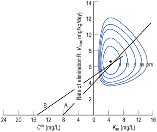
Since the dose/concentration relationship is non-linear, changes in dose do not result in proportional changes in plasma concentration (see Fig. 3.6B). Using the Michaelis–Menten model, if the plasma concentration is known at one dosage, then Vmax may be assumed to be the population average (7 mg/kg/day), since this is the more predictable parameter, and Km calculated using Eq. (15). The revised values of Km can then be used in Eq. (15) to estimate the new dosage required to produce a desired concentration. Alternatively, a nomogram may be used to assist in dose adjustments (Fig. 3.8).
Carbamazepine
Plasma concentration–response relationship when used in the treatment of epilepsy
Practical implications
Phenobarbital
Plasma concentration–response relationship
The sedation which commonly manifests early on in therapy becomes less with continued therapy.
Elimination
Phenobarbital is primarily (80%) metabolised by the liver, with approximately 20% being excreted unchanged in the urine. Elimination is a first-order process, but is relatively slow with a population average clearance of approximately 0.004 L/h/kg. However, as with theophylline, clearance in children is increased and is approximately twice the adult clearance. Applying Eqs. (6) and (8) to these population values gives an estimate of the half-life of the order of 5 days. This is much shorter in children and longer in the elderly.
Valproate
Elimination
As a result of the saturation of protein binding sites and the subsequent increase in the free fraction of the drug, clearance of the drug increases at higher concentrations. Therefore, there is a non-linear change in plasma concentration with dose (illustrated in Fig. 3.6C).
Lamotrigine, vigabatrin, gabapentin, tiagabine, topiramate, pregabalin, lacosamide and levetiracetam
Ciclosporin
Practical implications
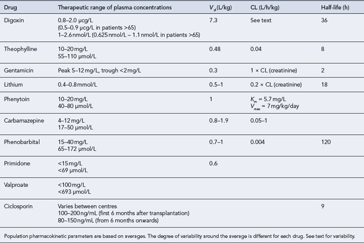
Summary pharmacokinetic data for drugs with therapeutic plasma concentrations are listed in Table 3.1
Case 3.1
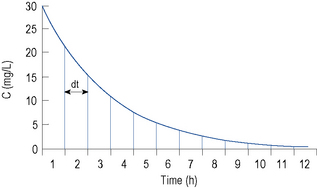
You are reviewing a formulary submission for a new formulation of a product, which has reportedly an improved side effect profile due to better absorption characteristics. However, there is conflicting evidence in the literature over the absorption of the new preparation. One paper, which is available to you, shows a concentration-time profile for the oral formulation after a single oral dose of 250 mg as in Table 3.2.
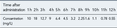
The paper also quotes an area under the curve (AUC) after a single i.v. dose of 200 mg as 87 mg/L/h.
Answers

Then add all the areas together (assume a value of 0 after 12 h)

Case 3.2
| Aspirin | 300 mg daily |
| Adcal D3 | Two tablets daily |
| Imdur | 60 mg daily |
| Simvastatin | 40 mg daily |
| Senna | 7.5 mg daily |
| Digoxin | 62.5 μcg daily |
She has been taking digoxin in a dose of 62.5 μcg daily for the last 3 weeks.
Questions


Case 3.3
| Urea | 31.6 mmol/L (3.2–7.5 mmol/L) |
| Creatinine | 168 μmol/L (71–133 μmol/L) |
Questions
Answers
Using the plasma levels reported:


Questions
Answers

The patient’s creatinine clearance (CrCL) is calculated using the Cockcroft and Gault equation:


Population data suggests that the volume of distribution (Vd) for lithium is 0.7 L/Kg.
Therefore, for this patient the volume of distribution:
The elimination rate constant ke is calculated:


Answers


The patient’s half-life (t1/2) = 7.8 h.


Case 3.6
| Pyridoxine | 12.5 mg daily |
| Rifater | four tablets daily |
| Phenytoin capsules | 350 mg daily |
One month after being started on this medication his phenytoin plasma level is measured as 7 mg/L
Answers
F, bioavailabilty; S, salt factor; Vmax, maximum rate of metabolism; Km, Michaelis-Menten constant.
Vmax = 7 mg/kg/day, Km = 5.7 mg/L, D = 350 mg, F = 1, S = 0.92.


The nearest practical dose would be 400 mg per day and a level checked again in 2 weeks.
Cockcroft D.W., Gault M.H. Prediction of creatinine clearance from plasma creatinine. Nephron. 1976;16:31-41.
Crist K.D., Nahata M.C., Ety J. Positive impact of a therapeutic drug monitoring program on total aminoglycoside dose and hospitalisation. Ther. Drug Monit.. 1987;9:306-310.
Department of Health. Estimated Glomerular Filtration Rate (eGFR). London: Department of Health Publications, 2006. Available from: //www.dh.gov.uk/en/Publicationsandstatistics/Publications/PublicationsPolicyAndGuidance/DH_4133020
Evans W.E., Shentag J.J., Jusko W.J., editors. Applied Pharmacokinetics, 3rd edn. Applied Therapeutics. Baltimore: Lippincott Williams & Wilkins. 1992:586-617.
Gjesdal K., Feyzi J., Olssen S.B. Digitalis: a dangerous drug in atrial fibrillation? Analysis of the SPORTIF III and V data. Heart. 2008;94:191-196.
McFadyen M.L., Miller R., Juta M., et al. The relevance of a first world therapeutic drug monitoring service to the treatment of epilepsy in third world conditions. S. Afr. Med. J.. 1990;78:587-590.
Nicolau D.P., Freeman C.D., Belliveau P.P., et al. Experience with a once daily aminoglycoside program administered to 2,184 adult patients. Antimicrob. Agents Chemother.. 1995;39:650-655.
Reid L.D., Horn J.R., McKenna D.A. Therapeutic drug monitoring reduces toxic drug reactions: a meta-analysis. Ther. Drug Monit. 1990;12:72-78.
Touw D.J., Neef C., Thomson A.H., et al. Cost-effectiveness of therapeutic drug monitoring: an update. Eur. J. Hosp. Pharm. Sci.. 2007;13:83-91.
Begg E.J., Barclay M.L., Duffull S.B. A suggested approach to once daily aminoglycoside dosing. Br. J. Clin. Pharmacol.. 1995;39:605-609.
Burton M.E., Shaw L.M., Schentag J.J. Applied Pharmacokinetics and Pharmacodynamics: Principles of Therapeutic Drug Monitoring, fourth ed. Baltimore: Lippincott Williams & Wilkins, 2006.
Dhillon S., Kostrzewski A. Clinical Pharmacokinetics. London: Pharmaceutical Press; 2006.
Elwes R.D.C., Binnie C.D. Clinical pharmacokinetics of newer antiepileptic drugs. Clin. Pharmacokinet.. 1996;30:403-415.
Jermain D.M., Crismon M.L., Martin E.S. Population pharmacokinetics of lithium. Clin. Pharmacokinet.. 1991;10:376-381.
Lemmer B., Bruguerolle B. Chronopharmacokinetics: are they clinically relevant? Clin. Pharmacokinet.. 1994;26:419-427.
Luke D.R., Halstenson C.E., Opsahl J.A., et al. Validity of creatinine clearance estimates in the assessment of renal function. Clin. Pharmacol. Ther.. 1990;48:503-508.
Rambeck B., Boenigk H.E., Dunlop A., et al. Predicting phenytoin dose: a revised nomogram. Ther. Drug Monit.. 1980;1:325-354.
Tserng K., King K.C., Takieddine F.N. Theophylline metabolism in premature infants. Clin. Pharmacol. Ther.. 1981;29:594-600.
Winter M.E. Basic Clinical Pharmacokinetics. Baltimore: Lippincott Williams & Wilkins; 2003.
Yukawa E. Optimisation of antiepileptic drug therapy: the importance of plasma drug concentration monitoring. Clin. Pharmacokinet.. 1996;31:120-130.