[level-membership-for-basic-science-category]
CHAPTER 8 Population and Mathematical Genetics
In this chapter, some of the more mathematical aspects of gene inheritance are considered, together with how genes are distributed and maintained at particular frequencies in populations. This subject constitutes what is known as population genetics. Genetics lends itself to a numerical approach, with many of the most influential and pioneering figures in human genetics having come from a mathematical background. They were particularly attracted by the challenges of trying to determine the frequencies of genes in populations and the rates at which they mutate. Much of this early work impinges on the specialty of medical genetics, and in particular on genetic counseling, and by the end of this chapter it is hoped that the reader will have gained an understanding of the following.
Allele Frequencies in Populations
The Hardy-Weinberg Principle
Consider an ‘ideal’ population in which there is an autosomal locus with two alleles, A and a, that have frequencies of p and q, respectively. These are the only alleles found at this locus, so that p + q = 100%, or 1. The frequency of each genotype in the population can be determined by construction of a Punnett square, which shows how the different genes can combine (Figure 8.1).
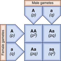
From Figure 8.1, it can be seen that the frequencies of the different genotypes are:
| Genotype | Phenotype | Frequency |
|---|---|---|
| AA | A | p2 |
| Aa | A | 2pq |
| Aa | a | q2 |
If there is random mating of sperm and ova, the frequencies of the different genotypes in the first generation will be as shown. If these individuals mate with one another to produce a second generation, Punnett square can again be used to show the different matings and their frequencies (Figure 8.2).
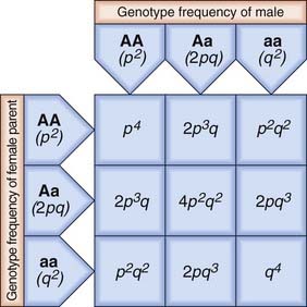
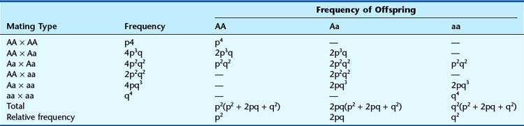
From Figure 8.2 the total frequency for each genotype in the second generation can be derived (Table 8.1). This shows that the relative frequency or proportion of each genotype is the same in the second generation as in the first. In fact, no matter how many generations are studied, the relative frequencies will remain constant. The actual numbers of individuals with each genotype will change as the population size increases or decreases, but their relative frequencies or proportions remain constant. This is the fundamental tenet of the Hardy-Weinberg principle. When studies confirm that the relative proportions of each genotype remain constant with frequencies of p2, 2pq, and q2, then that population is said to be in Hardy-Weinberg equilibrium for that particular genotype.
Factors that Can Disturb Hardy-Weinberg Equilibrium
Mutation
The validity of the Hardy-Weinberg principle is based on the assumption that no new mutations occur. If a particular locus shows a high mutation rate, then there will be a steady increase in the proportion of mutant alleles in a population. In practice, mutations do occur at almost all loci, albeit at different rates, but the effect of their introduction is usually balanced by the loss of mutant alleles due to reduced fitness of affected individuals. If a population is found to be in Hardy-Weinberg equilibrium, it is generally assumed that these two opposing factors have roughly equal effects. This is discussed further in the section that follows on the estimation of mutation rates.
Selection
Selection can act in the opposite direction by increasing fitness. For some autosomal recessive disorders there is evidence that heterozygotes show a slight increase in biological fitness compared with unaffected homozygotes—referred to as heterozygote advantage. The best understood example is sickle-cell disease, in which affected homozygotes have severe anemia and often show persistent ill-health (p. 159). However, heterozygotes are relatively immune to infection with Plasmodium falciparum malaria because their red blood cells undergo sickling and are rapidly destroyed when invaded by the parasite. In areas where this form of malaria is endemic, carriers of sickle-cell anemia (sickle cell trait), have a biological advantage compared with unaffected homozygotes. Therefore, in these regions the proportion of heterozygotes tends to increase relative to the proportions of normal and affected homozygotes, and Hardy-Weinberg equilibrium is disturbed.
Small Population Size
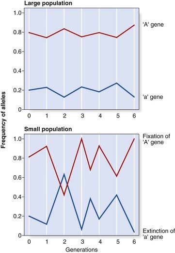
In a large population, the numbers of children produced by individuals with different genotypes, assuming no alteration in fitness for any particular genotype, will tend to balance out, so that gene frequencies remain stable. However, in a small population it is possible that by random statistical fluctuation one allele could be transmitted to a high proportion of offspring by chance, resulting in marked changes in allele frequency from one generation to the next, so that Hardy-Weinberg equilibrium is disturbed. This is known as random genetic drift. If one allele is lost altogether, it is said to be extinguished and the other allele is described as having become fixed (Figure 8.3).
Gene Flow (Migration)
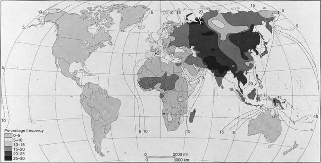
If new alleles are introduced into a population as a consequence of migration, with later intermarriage, a change in the relevant allele frequencies will result. This slow diffusion of alleles across racial or geographical boundaries is known as gene flow. The most widely quoted example is the gradient shown by the incidence of the B blood group allele throughout the world (Figure 8.4). This allele is thought to have originated in Asia and spread slowly westward as a result of admixture through invasion.
Validity of Hardy-Weinberg Equilibrium
| AA | 800 |
| Aa/aA | 185 |
| aa | 15 |
| Genotype | Observed | Expected |
|---|---|---|
| AA | 800 | 796.5 (p2 × 1000) |
| Aa/aA | 185 | 192 (2pq × 1000) |
| aa | 15 | 11.5 (q2 × 1000) |
These observed and expected values correspond closely and formal statistical analysis with a χ2 test would confirm that the observed values do not differ significantly from those expected if the population is in equilibrium.
| BB | 430 |
| Bb/bB | 540 |
| bb | 30 |
Using these values for p and q, the observed and expected genotype distributions can be compared:
| Genotype | Observed | Expected |
|---|---|---|
| BB | 430 | 490 (p2 × 1000) |
| Bb/bB | 540 | 420 (2pq × 1000) |
| bb | 30 | 90 (q2 × 1000) |
Applications of Hardy-Weinberg Equilibrium
Estimation of Carrier Frequencies
If the incidence of an AR disorder is known, it is possible to calculate the carrier frequency using some relatively simple algebra. For example, if the disease incidence is 1 in 10,000, then q2 =  and q =
  . Because p + q = 1, therefore p =
  . The carrier frequency can then be calculated as 2 ×
  ×
×  (i.e., 2pq), which approximates to 1 in 50. Thus, a rough approximation of the carrier frequency can be obtained by doubling the square root of the disease incidence. Approximate values for gene frequency and carrier frequency derived from the disease incidence can be extremely useful in genetic risk counseling (p. 266) (Table 8.2). However, if the disease incidence includes cases resulting from consanguineous relationships, then it is not valid to use the Hardy-Weinberg principle to calculate heterozygote frequencies because a high incidence of consanguinity disturbs the equilibrium by leading to a relative increase in the proportion of affected homozygotes.
Table 8.2 Approximate Values for Gene Frequency and Carrier Frequency Calculated from the Disease Incidence Assuming Hardy-Weinberg Equilibrium
| Disease Incidence (q2) | Gene Frequency (q) | Carrier Frequency (2pq) |
|---|---|---|
| 1/1000 | 1/32 | 1/16 |
| 1/2000 | 1/45 | 1/23 |
| 1/5000 | 1/71 | 1/36 |
| 1/10,000 | 1/100 | 1/50 |
| 1/50,000 | 1/224 | 1/112 |
| 1/100,000 | 1/316 | 1/158 |
 and p =
  . This means that the frequency of affected females (q2) and carrier females (2pq) is
  and
and  , respectively.
Estimation of Mutation Rates
Direct Method
If an autosomal dominant (AD) disorder shows full penetrance, and is therefore always expressed in heterozygotes, an estimate of its mutation rate can be made relatively easily by counting the number of new cases in a defined number of births. Consider a sample of 100,000 children, 12 of whom have a particular AD disorder such as achondroplasia (p. 93). Only two of these children have an affected parent, so that the remaining 10 must have acquired their disorder as a result of new mutations. Therefore 10 new mutations have occurred among the 200,000 genes inherited by these children (because each child inherits two copies of each gene), giving a mutation rate of 1 per 20,000 gametes per generation. In fact, this example is unusual because all new mutations in achondroplasia occur on the paternally derived chromosome 4; therefore the mutation rate is 1 per 10,000 in spermatogenesis and, as far as we know, zero in oogenesis.
Why is it Helpful to Know Mutation Rates?
Estimation of Gene Size
If a disorder has a high mutation rate the gene may be large. Alternatively, it may contain a high proportion of GC residues and be prone to copy error, or contain a high proportion of repeat sequences (p. 23), which could predispose to misalignment in meiosis resulting in deletion and duplication.
Why are Some Genetic Disorders More Common than Others?
Small Populations
Several rare AR disorders show a relatively high incidence in certain population groups (Table 8.3). High allele frequencies are usually explained by the combination of a founder effect together with social, religious, or geographical isolation—hence the term genetic isolates. In some situations, genetic drift may have played a role.
Table 8.3 Rare Recessive Disorders that Are Relatively Common in Certain Groups of People
| Group | Disorder | Clinical Features |
|---|---|---|
| Finns | Congenital nephrotic syndrome | Edema, proteinuria, susceptibility to infection |
| Aspartylglycosaminuria | Progressive mental and motor deterioration, coarse features | |
| Mulibrey nanism | Muscle, liver, brain and eye involvement | |
| Congenital chloride diarrhea | Reduced Cl– absorption, diarrhea | |
| Diastrophic dysplasia | Progressive epiphyseal dysplasia with dwarfism and scoliosis | |
| Amish | Cartilage–hair hypoplasia | Dwarfism, fine, light-colored and sparse hair |
| Ellis–van Creveld syndrome | Dwarfism, polydactyly, congenital heart disease | |
| Glutaric aciduria type 1 | Episodic encephalopathy and cerebral palsy-like dystonia | |
| Hopi and San Blas Indians | Albinism | Lack of pigmentation |
| Ashkenazi Jews | Tay-Sachs disease | Progressive mental and motor deterioration, blindness |
| Gaucher disease | Hepatosplenomegaly, bone lesions, skin pigmentation | |
| Dysautonomia | Indifference to pain, emotional lability, lack of tears, hyperhidrosis | |
| Karaite Jews | Werdnig-Hoffmann disease | Infantile spinal muscular atrophy |
| Afrikaners | Sclerosteosis | Tall stature, overgrowth of craniofacial bones with cranial nerve palsies, syndactyly |
| Lipoid proteinosis | Thickening of skin and mucous membranes | |
| Ryukyan islands (off Japan) | ‘Ryukyan’ spinal muscular atrophy | Muscle weakness, club foot, scoliosis |
Founder effects can also be observed in AD disorders. Variegate porphyria, which is characterized by photosensitivity and drug-induced neurovisceral disturbance, has a high incidence in the Afrikaner population of South Africa, believed to be due to one of the early Dutch settlers having transmitted the condition to a large number of descendants (p. 109).
Large Populations
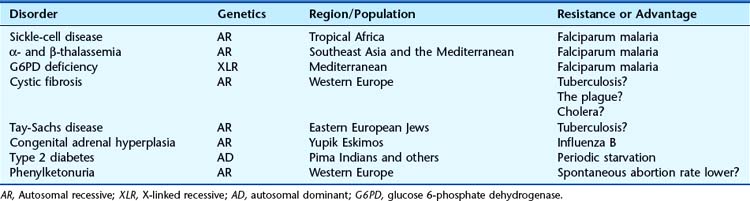
When a serious AR disorder, resulting in reduced fitness in affected homozygotes, has a high incidence in a large population, the explanation is presumed to lie in either a very high mutation rate and/or a heterozygote advantage. The latter explanation is the more probable for most AR disorders (Table 8.4).
Table 8.4 Presumed Increased Resistance in Heterozygotes that could Account for the Maintenance of Various Genetic Disorders in Certain Populations
Heterozygote Advantage
For sickle cell (SC) anemia (p. 159) and thalassemia (p. 161), there is very good evidence that heterozygote advantage results from reduced susceptibility to Plasmodium falciparum malaria, as explained in Chapter 10. Americans of Afro-Caribbean origin are no longer exposed to malaria, so it would be expected that the frequency of the SC allele in this group would gradually decline. However, the predicted rate of decline is so slow that it will be many generations before it is detectable.
For several AR disorders the mechanisms proposed for heterozygote advantage are largely speculative (see Table 8.4). The discovery of the cystic fibrosis (CF) gene, with the subsequent elucidation of the role of its protein product in membrane permeability (p. 301), supports the hypothesis of selective advantage through increased resistance to the effects of gastrointestinal infections, such as cholera and dysentery, in the heterozygote. This relative resistance could result from reduced loss of fluid and electrolytes. It is likely that this selective advantage was of greatest value several hundred years ago when these infections were endemic in Western Europe. If so, a gradual decline in the incidence of CF would be expected. However, if this theory is correct one has to ask why CF has not become relatively common in other parts of the world where gastrointestinal infections are endemic, particularly the tropics; in fact, the opposite is the case, for CF is rare in these regions.
An alternative, but speculative, mechanism for the high incidence of a condition such as CF is that the mutant allele is preferentially transmitted at meiosis. This type of segregation distortion, whereby an allele at a particular locus is transmitted more often than would be expected by chance (i.e., in more than 50% of gametes), is referred to as meiotic drive. Firm evidence for this phenomenon in CF is lacking, although it has been demonstrated in the AD disorder myotonic dystrophy (p. 295).
Genetic Polymorphism
In humans, at least 30% of structural gene loci are polymorphic, with each individual being heterozygous at between 10% and 20% of all loci. Known polymorphic protein systems include the ABO blood groups (p. 205) and many serum proteins, which may exhibit polymorphic electrophoretic differences—or isozymes.
DNA polymorphisms, including SNPs, have been crucial to positional cloning, gene mapping, and isolation of many disease genes (p. 75). They are also used in gene tracking (p. 70) in the clinical context of presymptomatic tests, prenatal diagnosis and carrier detection for many single-gene disorders where direct mutation analysis may not be possible. The value of a particular polymorphic system is assessed by determining its polymorphic information content (PIC). The higher the PIC value, the more likely it is that a polymorphic marker will be of value in linkage analysis and gene tracking.
Segregation Analysis
Autosomal Recessive Inheritance
For disorders thought to follow AR inheritance, formal segregation analysis is much more difficult. This is because some couples who are both carriers will by chance not have affected children, therefore not feature in ascertainment. To illustrate this, consider 64 possible sibships of size 3 in which both parents are carriers, drawn from a large hypothetical population (Table 8.5). The sibship structure shown in Table 8.5 is that which would be expected, on average.
Table 8.5 Expected Sibship Structure in a Hypothetical Population that Contains 64 Sibships Each of Size 3, in Which Both Parents are Carriers of an Autosomal Recessive Disorder. If No Allowance Is Made for Truncate Ascertainment, in that the 27 Sibships with No Affected Cases Will Not Be Ascertained, Then a Falsely High Segregation Ratio of 48/111 (= 0.43) Will Be Obtained
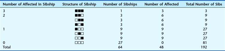
In this population, on average, 27 of the 64 sibships will not contain any affected individuals. This can be calculated simply by cubing  —i.e.,
  ×
×  ×
×  =
=  . Therefore, when the families are analyzed, these 27 sibships containing only healthy individuals will not be ascertained—referred to as incomplete ascertainment. If this is not taken into account, a falsely high segregation ratio of 0.43 will be obtained instead of the correct value of 0.25.
Mathematical methods have been devised to cater for incomplete ascertainment, but analysis is usually further complicated by problems associated with achieving full or complete ascertainment. In practice ‘proof’ of AR inheritance requires accurate molecular or biochemical markers for carrier detection. Affected siblings (especially when at least one is female) born to unaffected parents usually suggests AR inheritance, but somatic and germline parental mosaicism (p. 121), non-paternity, and other possibilities need to be considered. There are some good examples of conditions originally reported to follow AR inheritance but subsequently shown to be dominant with germline or somatic mosaicism; for example, osteogenesis imperfecta and pseudoachondroplasia. However, a high incidence of parental consanguinity undoubtedly provides strong supportive evidence for AR inheritance, as first noted by Bateson and Garrod in 1902 (pp. 7, 113).
Genetic Linkage
Mendel’s third law—the principle of independent assortment—states that members of different gene pairs assort to gametes independently of one another (p. 5). Stated more simply, the alleles of genes at different loci segregate independently. Although this is true for genes on different chromosomes, it is not always true for genes that are located on the same chromosome (i.e., close together, or syntenic).
Two loci positioned adjacent, or close, to each other on the same chromosome, will tend to be inherited together, and are said to be linked. The closer they are, the less likely they will be separated by a crossover, or recombination, during meiosis I (Figure 8.5).
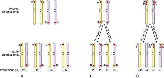
Linked alleles on the same chromosome are said to be in coupling, whereas those on opposite homologous chromosomes are described as being in repulsion. This is known as the linkage phase. Thus in the parental chromosomes in Figure 8.5, C, A and B, as well as a and b, are in coupling, whereas A and b, as well as a and B, are in repulsion.
Centimorgans
The human genome has been estimated by recombination studies to be about 3000 cM in length in males. Because the physical length of the haploid human genome is approximately 3 × 10⁹ bp, 1 cM corresponds to approximately 106 bp (1 Mb or 1000 kb). However, the relationship between linkage map units and physical length is not linear. Some chromosome regions appear to be particularly prone to recombination—so-called ‘hotspots’—and recombination occurs less often during meiosis in males than in females, in whom the genome ‘linkage’ length has been estimated to be 4200 cM. Generally, in humans one or two recombination events take place between each pair of homologous chromosomes in meiosis I, with a total of ~40 across the entire genome. Recombination events are rare close to the centromeres but relatively common in telomeric regions.
Linkage Analysis
Linkage analysis has proved invaluable for mapping genes (see Chapter 5). It is based on studying the segregation of the disease with polymorphic markers from each chromosome—preferably in large families. Eventually a marker will be identified that co-segregates with the disease more often than would be expected by chance (i.e., the marker and disease locus are linked). The mathematical analysis tends to be very complex, particularly if many closely adjacent markers are being used, as in multipoint linkage analysis. However, the underlying principle is relatively straightforward and involves the use of likelihood ratios, the logarithms of which are known as LOD scores (logarithm of the odds).
LOD Scores
For example, when a research paper reports that linkage of a disease with a DNA marker has been identified with a LOD score (Z) of 4 at recombination fraction (θ) 0.05, this means that the results, in the families studied, indicate that it is 10,000 (104) times more likely that the disease and marker loci are closely linked (i.e., 5 cM apart) than that they are not linked. It is generally agreed that a LOD score of +3 or more is confirmation of linkage. This would yield a ratio of 1000 to 1 in favor of linkage; however, because there is a prior probability of only 1 in 50 that any two given loci are linked, a LOD score of +3 means that the overall probability that the loci are linked is approximately 20 to 1—i.e., [1000 ×  ]:1. The importance of taking prior probabilities into account in probability theory is discussed in the section on Bayes’ theorem (p. 339).
A ‘Simple’ Example
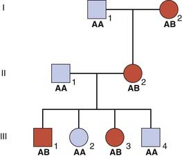
Consider a three-generation family in which several members have an AD disorder (Figure 8.6). A and B are alleles at a locus that is being tested for linkage to the disease locus.
To confirm linkage other families would have to be studied by pooling all the results until a LOD score of +3 or greater was obtained. A LOD score of −2 or less is taken as proof that the loci are not linked. This less stringent requirement for proof of non-linkage (i.e., a LOD score of −2 compared with +3 for proof of linkage) is due to the high prior probability of  that any two loci are not linked.
Multipoint Linkage Analysis
Using this approach the results of linkage studies with the various markers are analyzed by a computer program that calculates the overall likelihood of the position of the disease locus in relation to the marker loci. The results are presented in the form of a likelihood ratio known as a location score. This is calculated for different positions of the disease locus and a graph is drawn up of location score against map distance (Figure 8.7). On this graph the peaks represent possible positions of the disease locus, with the tallest peak being the most probable location. The troughs represent the positions of the polymorphic marker loci.
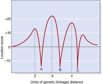
Multipoint linkage analysis is used to define the smallest possible interval in which a disease locus is located, so that physical mapping methods can then be applied to isolate the disease gene (see Chapter 5).
Autozygosity Mapping
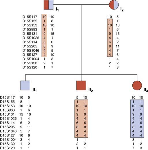
This ingenious form of linkage analysis has been used to map many rare AR disorders. Autozygosity occurs when individuals are homozygous at particular loci by descent from a common ancestor. In an inbred pedigree containing two or more children with a rare AR disorder, it is very likely that the children will be homozygous not only at the disease locus but also at closely linked loci. In other words, all affected relatives in an inbred family will be homozygous for markers within the region surrounding the disease locus. Thus a search can be made for shared areas of homozygosity in affected relatives using highly polymorphic markers such as microsatellites (p. 69). In a pedigree with a relatively large number of affected individuals, only a small number of shared homozygous regions will be identified; one of these can be expected to harbor the relevant disease locus, which can then be isolated using physical mapping strategies.
Autozygosity mapping can be applied in both small inbred families (Figure 8.8) and in genetic isolates (p. 133) with a shared common genetic ancestry (e.g., the Old Order Amish). It is a particularly powerful technique in large inbred families in which more than one branch has affected individuals. Several of the genes that cause AR sensorineural hearing loss have been mapped in this way, as well as a number of skeletal dysplasias and primary microcephalies, for example.
Linkage Disequilibrium
The rationale for studying allelic association in populations is based on the assumption that a mutation occurred in a founder case some generations previously and is still causative of the disease. If this is true, the pattern of markers in a small region close to the mutation will have been maintained and thus constitutes what is termed the founder haplotype. The underlying principles used in mapping are the same as those for linkage analysis in families, the difference being the degree of relatedness of the individuals under study. In the pedigree shown in Figure 8.6, support was obtained for linkage of the disease gene with the B marker allele. Assume that further studies confirm linkage of these loci and that the A and B alleles have an equal frequency of 0.5. It would be reasonable to expect that the disease gene would be in coupling with allele A in approximately 50% of families and with allele B in the remaining 50%. If, however, the disease allele was found to be in coupling exclusively with one particular marker allele, this would be an example of linkage disequilibrium.
The demonstration of linkage disequilibrium in a particular disease suggests that the mutation causing the disease has occurred relatively recently and that the marker locus studied is very closely linked to the disease locus. There may be pitfalls, however, in interpreting haplotype data that suggest linkage disequilibrium. Other possible reasons for linkage disequilibrium include: (1) the rapid growth of genetically isolated populations leading to large regions of allelic association throughout the genome; (2) selection, whereby particular alleles enhance or diminish reproductive fitness; and (3) population admixture, where population subgroups with different patterns of allele frequencies are combined into a single study. Allowance for the latter problem can be made by using family-based controls and analyzing the transmission of alleles using a method called the transmission/disequilibrium test. This uses the fact that transmitted and non-transmitted alleles from a given parent are paired observations, and examines the preferential transmission of one allele over the other in all heterozygous parents. The technique has been applied, amongst others, to studies based on sibling pairs that are discordant for the disease or condition under study.
Medical and Societal Intervention
Recent developments in molecular biology, such as the human genome project (p. 9) and pilot studies using gene therapy (p. 350), have reawakened concern that future generations could have to cope with an ever increasing burden of genetic disease. The term eugenics was first used by Charles Darwin’s cousin, Francis Galton, to refer to the improvement of a population by selective breeding. The notion that this should be applied to human populations became popular during the early years of the twentieth century, culminating in the horrifying practices of Nazi Germany. Ensuing revulsion led to the abandonment of eugenic programs in humans, with universal condemnation and agreement that such programs have no place in modern medical practice. Sadly, however, these practices have continued by groups engaged in territorial conflicts—somewhat sanitized by the term ‘ethnic cleansing.’
Doctors caring for patients and families with hereditary disease inevitably give priority to treatment and improving survival. By so doing biological fitness may be increased, leading to increased numbers of ‘bad genes’ in society, potentially adding adversely to humanity’s future genetic load. Such long-term consequences generally carry no weight, but the approach has sometimes been interpreted as dysgenic.
AD Disorders
Alternatively, if successful treatment became available for all patients with a serious AD disorder that at present is associated with a marked reduction in genetic fitness, there would be an immediate increase in the frequency of the disease gene followed by a more gradual leveling off at a new equilibrium level. If, at one time, all those with a serious AD disorder died in childhood (f = 0), then the incidence of affected individuals would be 2µ. If treatment raised the fitness from 0 to 0.9, the incidence of affected children in the next generation would rise to 2µ due to new mutations plus 1.8µ inherited, which equals 3.8µ. Eventually a new equilibrium would be reached, by which time the disease incidence would have risen tenfold to 20µ. This can be calculated relatively easily with the formula µ = [I(1 − f)]/2 (p. 133), which can also be expressed as I = 2µ/(1 – f). The net result would be that the proportion of affected children who died would be lower (from 100% down to 10%), but the total number affected would be much greater, although the actual number who died from the disease would remain unchanged at 2µ.
X-Linked Recessive Disorders
When considering the effects of selection against these disorders, it is necessary to take into account the fact that a large proportion of the relevant genes are present in entirely healthy female carriers, who are often unaware of their carrier status. For a very serious condition, such as Duchenne muscular dystrophy (p. 307), with fitness equal to 0 in affected males, selection will have no effect unless female carriers choose to limit their families. If all female carriers opted not to have any children, the incidence would be reduced by two-thirds (i.e., from 3µ to µ).
A much more plausible possibility is that effective treatment will be forthcoming for these disorders. This will result in a steady increase in the disease incidence. For example, an increase in fitness from 0 to 0.5 will lead to a doubling of the disease incidence by the time a new equilibrium has been established. This can be calculated using the formula µ = [IM(1 − f)]/3 (p. 133).
Allison AC. Protection afforded by sickle-cell trait against subtertian malarial infection. BMJ. 1954;i:290-294.
Emery AEH. Methodology in medical genetics, 2nd ed. Edinburgh: Churchill Livingstone; 1986.
Francomano CA, McKusick VA, Biesecker LG, Medical genetic studies in the Amish: historical perspective, eds, Am J Med Genet C Semin Med Genet; 121:2003:1-4
Haldane JBS. The rate of spontaneous mutation of a human gene. J Genet. 1935;31:317-326.
The first estimate of the mutation rate for hemophilia using an indirect method.
Hardy GH. Mendelian proportions in a mixed population. Science. 1908;28:49-50.
Khoury MJ, Beaty TH, Cohen BH. Fundamentals of genetic epidemiology. New York: Oxford University Press; 1993.
A comprehensive textbook of population genetics and its areas of overlap with epidemiology.
Ott J. Analysis of human genetic linkage. Baltimore: Johns Hopkins University Press; 1991.
A detailed mathematical explanation of linkage analysis.
Vogel F, Motulsky AG. Human genetics, problems and approaches, 3d ed. Berlin: Springer; 1997.
The definitive textbook of human genetics with extensive coverage of mathematical aspects.
Elements
[/level-membership-for-basic-science-category][not-level-membership-for-basic-science-category]
CHAPTER 8 Population and Mathematical Genetics
In this chapter, some of the more mathematical aspects of gene inheritance are considered, together with how genes are distributed and maintained at particular frequencies in populations. This subject constitutes what is known as population genetics. Genetics lends itself to a numerical approach, with many of the most influential and pioneering figures in human genetics having come from a mathematical background. They were particularly attracted by the challenges of trying to determine the frequencies of genes in populations and the rates at which they mutate. Much of this early work impinges on the specialty of medical genetics, and in particular on genetic counseling, and by the end of this chapter it is hoped that the reader will have gained an understanding of the following.
Allele Frequencies in Populations
The Hardy-Weinberg Principle
Consider an ‘ideal’ population in which there is an autosomal locus with two alleles, A and a, that have frequencies of p and q, respectively. These are the only alleles found at this locus, so that p + q = 100%, or 1. The frequency of each genotype in the population can be determined by construction of a Punnett square, which shows how the different genes can combine (Figure 8.1).
From Figure 8.1, it can be seen that the frequencies of the different genotypes are:
| Genotype | Phenotype | Frequency |
|---|---|---|
| AA | A | p2 |
| Aa | A | 2pq |
| Aa | a | q2 |
If there is random mating of sperm and ova, the frequencies of the different genotypes in the first generation will be as shown. If these individuals mate with one another to produce a second generation, Punnett square can again be used to show the different matings and their frequencies (Figure 8.2).
From Figure 8.2 the total frequency for each genotype in the second generation can be derived (Table 8.1). This shows that the relative frequency or proportion of each genotype is the same in the second generation as in the first. In fact, no matter how many generations are studied, the relative frequencies will remain constant. The actual numbers of individuals with each genotype will change as the population size increases or decreases, but their relative frequencies or proportions remain constant. This is the fundamental tenet of the Hardy-Weinberg principle. When studies confirm that the relative proportions of each genotype remain constant with frequencies of p2, 2pq, and q2, then that population is said to be in Hardy-Weinberg equilibrium for that particular genotype.
Factors that Can Disturb Hardy-Weinberg Equilibrium
Mutation
The validity of the Hardy-Weinberg principle is based on the assumption that no new mutations occur. If a particular locus shows a high mutation rate, then there will be a steady increase in the proportion of mutant alleles in a population. In practice, mutations do occur at almost all loci, albeit at different rates, but the effect of their introduction is usually balanced by the loss of mutant alleles due to reduced fitness of affected individuals. If a population is found to be in Hardy-Weinberg equilibrium, it is generally assumed that these two opposing factors have roughly equal effects. This is discussed further in the section that follows on the estimation of mutation rates.
Selection
Selection can act in the opposite direction by increasing fitness. For some autosomal recessive disorders there is evidence that heterozygotes show a slight increase in biological fitness compared with unaffected homozygotes—referred to as heterozygote advantage. The best understood example is sickle-cell disease, in which affected homozygotes have severe anemia and often show persistent ill-health (p. 159). However, heterozygotes are relatively immune to infection with Plasmodium falciparum malaria because their red blood cells undergo sickling and are rapidly destroyed when invaded by the parasite. In areas where this form of malaria is endemic, carriers of sickle-cell anemia (sickle cell trait), have a biological advantage compared with unaffected homozygotes. Therefore, in these regions the proportion of heterozygotes tends to increase relative to the proportions of normal and affected homozygotes, and Hardy-Weinberg equilibrium is disturbed.
Small Population Size
In a large population, the numbers of children produced by individuals with different genotypes, assuming no alteration in fitness for any particular genotype, will tend to balance out, so that gene frequencies remain stable. However, in a small population it is possible that by random statistical fluctuation one allele could be transmitted to a high proportion of offspring by chance, resulting in marked changes in allele frequency from one generation to the next, so that Hardy-Weinberg equilibrium is disturbed. This is known as random genetic drift. If one allele is lost altogether, it is said to be extinguished and the other allele is described as having become fixed (Figure 8.3).
Gene Flow (Migration)
If new alleles are introduced into a population as a consequence of migration, with later intermarriage, a change in the relevant allele frequencies will result. This slow diffusion of alleles across racial or geographical boundaries is known as gene flow. The most widely quoted example is the gradient shown by the incidence of the B blood group allele throughout the world (Figure 8.4). This allele is thought to have originated in Asia and spread slowly westward as a result of admixture through invasion.
Validity of Hardy-Weinberg Equilibrium
| AA | 800 |
| Aa/aA | 185 |
| aa | 15 |
| Genotype | Observed | Expected |
|---|---|---|
| AA | 800 | 796.5 (p2 × 1000) |
| Aa/aA | 185 | 192 (2pq × 1000) |
| aa | 15 | 11.5 (q2 × 1000) |
These observed and expected values correspond closely and formal statistical analysis with a χ2 test would confirm that the observed values do not differ significantly from those expected if the population is in equilibrium.
| BB | 430 |
| Bb/bB | 540 |
| bb | 30 |
Using these values for p and q, the observed and expected genotype distributions can be compared:
| Genotype | Observed | Expected |
|---|---|---|
| BB | 430 | 490 (p2 × 1000) |
| Bb/bB | 540 | 420 (2pq × 1000) |
| bb | 30 | 90 (q2 × 1000) |
Applications of Hardy-Weinberg Equilibrium
Estimation of Carrier Frequencies
If the incidence of an AR disorder is known, it is possible to calculate the carrier frequency using some relatively simple algebra. For example, if the disease incidence is 1 in 10,000, then q2 = and q = . Because p + q = 1, therefore p = . The carrier frequency can then be calculated as 2 × × (i.e., 2pq), which approximates to 1 in 50. Thus, a rough approximation of the carrier frequency can be obtained by doubling the square root of the disease incidence. Approximate values for gene frequency and carrier frequency derived from the disease incidence can be extremely useful in genetic risk counseling (p. 266) (Table 8.2). However, if the disease incidence includes cases resulting from consanguineous relationships, then it is not valid to use the Hardy-Weinberg principle to calculate heterozygote frequencies because a high incidence of consanguinity disturbs the equilibrium by leading to a relative increase in the proportion of affected homozygotes.
Table 8.2 Approximate Values for Gene Frequency and Carrier Frequency Calculated from the Disease Incidence Assuming Hardy-Weinberg Equilibrium
| Disease Incidence (q2) | Gene Frequency (q) | Carrier Frequency (2pq) |
|---|---|---|
| 1/1000 | 1/32 | 1/16 |
| 1/2000 | 1/45 | 1/23 |
| 1/5000 | 1/71 | 1/36 |
| 1/10,000 | 1/100 | 1/50 |
| 1/50,000 | 1/224 | 1/112 |
| 1/100,000 | 1/316 | 1/158 |
Estimation of Mutation Rates
Direct Method
If an autosomal dominant (AD) disorder shows full penetrance, and is therefore always expressed in heterozygotes, an estimate of its mutation rate can be made relatively easily by counting the number of new cases in a defined number of births. Consider a sample of 100,000 children, 12 of whom have a particular AD disorder such as achondroplasia (p. 93). Only two of these children have an affected parent, so that the remaining 10 must have acquired their disorder as a result of new mutations. Therefore 10 new mutations have occurred among the 200,000 genes inherited by these children (because each child inherits two copies of each gene), giving a mutation rate of 1 per 20,000 gametes per generation. In fact, this example is unusual because all new mutations in achondroplasia occur on the paternally derived chromosome 4; therefore the mutation rate is 1 per 10,000 in spermatogenesis and, as far as we know, zero in oogenesis.
