CHAPTER 19 Physiologic Evaluation of the Brain with Magnetic Resonance Imaging
Diffusion-Weighted Imaging
DWI characterizes differences in the brownian motion of water molecules, depending on their local environment. In bulk, water molecules can move freely in any direction. Biologic systems typically impede the free motion of water in one or more directions. Thus, cellular structure, permeability barriers, and various macromolecules within the brain parenchyma may all restrict the free diffusion of water molecules. Normally, restriction tends to be greater within the intracellular space than within the extracellular space1; thus, extracellular water molecules can diffuse more freely than intracellular molecules.
Physics
The imaging technique most often used for DWI is an echo planar imaging (EPI) sequence. In EPI, two separate and equal magnetic gradients are applied to opposite sides of the radiofrequency (RF) pulse during image acquisition. Use of these bipolar pulsed gradients allows detection of diffusional motion by changes in the magnitude of the moving spins from phase dispersion. Water molecules that do not travel significantly between excitation pulse and read pulse will not dephase significantly and will therefore retain much of their initial signal. Thus, in pathologic states, the increased signal on DWI reflects an abnormal decrease in water diffusivity, typically caused by either loss of normal extracellular space (as seen in cytotoxic edema) or the presence of a highly viscous, proteinaceous, or cellular environment.1,2 It is worth noting that loss of signal is not due to travel of water from one imaging voxel to another, but rather motion within the voxels themselves. Indeed, the average motion of a water molecule at 40°C is 2.5 × 10⁻³ mm2/sec, which translates into motion of 22 µm in 100 msec; this is considerably smaller than the typical 1- to 2-mm voxel dimension.3
The magnitude of diffusion sensitization of DWI is determined by the “b-value,” which in turn is related to the duration, strength, and time interval between the magnetic gradients. Therefore, higher b-values confer more sensitive DWI and thus yield improved contrast and ability to identify areas of water restriction; however, higher b-values also result in loss of signal, as well as noisier images, which may then have reduced utility. The b-value that is typically used in clinical assessment is approximately 800 to 1000 sec/mm2,4 but with certain applications, such as vertebral imaging or characterization of intracranial tumors, b-values may range from 500 to 2000 sec/mm2 or greater.
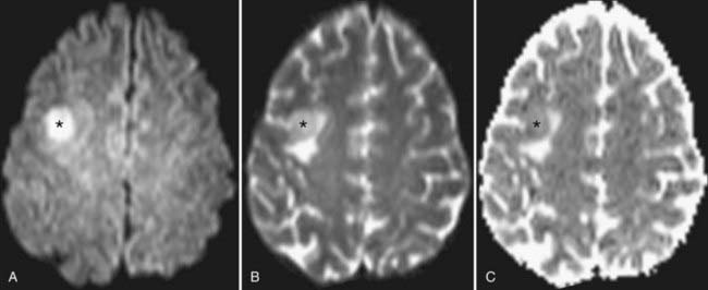
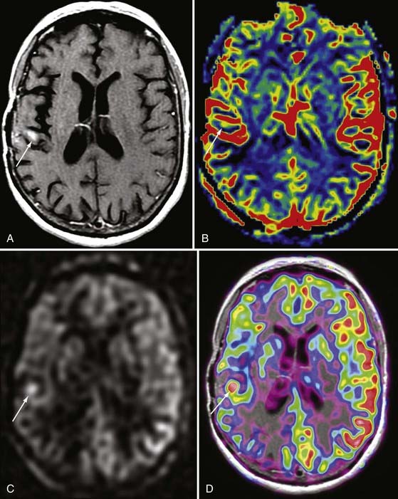
The rate of diffusional motion is characterized by the apparent diffusion coefficient (ADC). This quantitative estimate of diffusivity can be achieved by acquiring two sets of images with different b-values, which can eliminate the effects of spin density and T1 and T2 relaxation. In clinical practice, one of the b-values would measure approximately 1000 sec/mm2, as indicated earlier. The other b-value is typically 0 sec/mm2, which reflects an image that does not have any motion-probing gradient applied (yielding so-called B0 images). ADC maps quantify differences between B0 and B1000 images and therefore nullify “T2 shine-through,” a condition in which high B1000 signal is primarily due to high T2 signal rather than water restriction (Fig. 19-1). Thus, true restricted diffusion, as seen with acute ischemia, will demonstrate high signal on DWI and corresponding low signal on ADC maps.1
Clinical Uses and Applications
In clinical use, diffusion images are acquired in at least three directions, with the resulting images mathematically averaged to generate the trace image in which regions of normal white matter and gray matter appear fairly uniform. The normal brain shows slight variation in diffusion signal based on cellular structure. Gray matter has marginally higher signal on DWI, probably reflecting differing T2 properties rather than true differences in the ADC. Areas that are essentially water (most notably CSF) are dark on DWI sequences because of the free motion of water molecules in bulk water.5
The most completely characterized application of DWI is for the diagnosis and management of patients with acute cerebral ischemia. When perfusion does not meet the metabolic demand of territorial parenchyma, energy-dependent sodium-potassium adenosine triphosphatase ion pumps may fail. The resulting ion flux leads to the accumulation of water within the intracellular compartment (cytotoxic edema). Neuronal swelling crowds the extracellular space, with resulting restricted motion of extracellular water molecules that is manifest as high DWI signal; these changes may be seen within minutes of tissue infarction. Normal brain ADC values range from approximately 740 to 840 × 10−6 mm2/sec, with considerable overlap between white matter and gray matter values.6 Parenchyma with ADC values of less than 500 to 550 × 10−6 mm2/sec is almost certainly in the process of irreversible infarction. Intermediate ADC values (550 to 700 × 10−6 mm2/sec) may reflect parenchyma that is ischemic yet still viable; it is this tissue that may be potentially salvageable with appropriate intervention. Although DWI is frequently identified as the most sensitive sequence for detecting infarction, other complementary sequences (such as the perfusion sequences described later) can help define an apparent impending infarction and define tissue at risk for infarction, the so-called ischemic penumbra.7,8
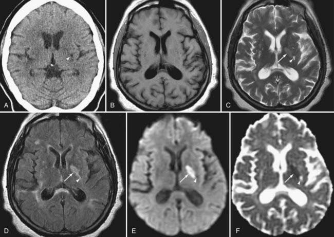
As infarcts age, the ADC and DWI patterns mature at differing rates. Although both become abnormal within minutes, the ADC increases from low signal to isointensity more rapidly, in most instances within 5 to 14 days. The ADC then continues to rise over the ensuing weeks to remain positive for the life of the patient, corresponding with encephalomalacia. DWI normalizes more slowly. It may reach isointensity with surrounding brain as long as 4 to 5 weeks after the infarction, and it will take even longer for signal to decline further in the setting of encephalomalacia (Fig. 19-2).
Certain intracranial neoplasms demonstrate restricted diffusion. Many of these neoplasms are tumors that are high in cellularity, with resulting high signal on DWI and low signal on the ADC map (i.e., true diffusion restriction). Examples include lymphoma, medulloblastoma, and portions of high-grade gliomas. Some tumors demonstrate restriction without high cellularity. Hence, although both epidermoid cysts and arachnoid cysts closely follow fluid intensity on T1, T2, and fluid-attenuated inversion recovery (FLAIR) sequences, the high DWI signal and heterogeneous low signal on the ADC map conferred by desquamated debris allow confident diagnosis of an epidermoid. Arachnoid cysts, which instead contain simple fluid, demonstrate facilitated diffusion and therefore have the opposite diffusion pattern (low DWI signal and high ADC signal).9
Brain abscesses are typically peripherally enhancing lesions that are usually surrounded by significant vasogenic edema. Occasionally, these lesions can be difficult to differentiate from other peripherally enhancing masses such as necrotic tumors. The central cavity of an abscess demonstrates high signal on DWI and low signal on ADC maps. The restricted diffusion is most likely attributed to the high viscosity of proteinaceous fluid and the hypercellularity of inflammatory cells.10–12
Seizure activity can induce changes in water diffusivity because of cellular swelling and fluctuation in extracellular fluid. Cortical restricted diffusion has been seen with prolonged seizure activity, presumably caused by an imbalance between oxygen delivery and consumption.13 Focal parenchymal changes in the postictal state can be seen as hyperintense signal changes on T2-weighted sequences with variability in DWI signal. In the setting of ischemia related to seizure activity, DWI may initially demonstrate restricted diffusion as a result of cytotoxic edema, but the restricted diffusion can later progress to decreased diffusion signal, which may represent gliosis of the involved tissue.14
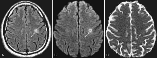
DWI also aids in the diagnosis and further characterization of other disease processes. Restricted diffusion can be seen in zones of active demyelination in such disease processes as multiple sclerosis and progressive multifocal leukoencephalopathy (Fig. 19-3), in areas of active inflammation typically seen in the medial temporal lobes in herpes simplex encephalitis, in the anterior deep gray nuclei of the basal ganglia and along a discontinuous cortical ribbon in Creutzfeldt-Jacob disease, in some phases of hemorrhage, and in some encephalopathies and leukodystrophies.1,9
Pitfalls and Limitations
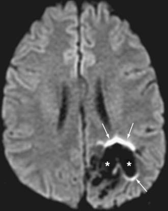
EPI techniques allow ultrafast acquisition times, thereby almost eliminating motion artifact. However, the long echo train lengths needed to obtain the data render these sequences sensitive to both chemical shifts and magnetic susceptibility. Lipid suppression can be used to resolve some effects of chemical shift. Eddy currents result from the use of rapidly alternating gradients; these currents may result in significant distortion or misregistration between directional acquisition, which translates into blurring and loss of soft tissue contrast in the resulting trace image. Traditional DWI is prone to areas of susceptibility, most notably about the skull base, paranasal sinuses, and petrous bone, where air-bone-tissue interfaces are present.5,15,16 In addition, the presence of paramagnetic and ferromagnetic material such as blood products or metal from surgery, trauma, or dental hardware can produce significant artifact, seen as ghosting, image distortion, and susceptibility artifact (Fig. 19-4). Newer techniques (periodically rotated overlapping parrallel lines with enhanced reconstruction [PROPELLER], BLADE, and others) use a rotating acquisition frame to minimize the effect of such artifacts and increase the sensitivity for abnormalities in previously challenging areas; however, these sequences may be associated with a significant increase in scanning time.
Diffusion Tensor Imaging and Tractography
Physics
As mentioned in the discussion on DWI, the water motion illustrated on diffusion sequences is predominantly extracellular, and the vector of motion tends to parallel the white matter tracts. In DTI, the acquisition of at least six directions allows mathematical construction of a tensor ellipsoid whose major axis points in the direction of the dominant fiber tract within a voxel.17 In voxels in which white matter tracts are homogeneous and nearly colinear, this ellipsoid is thin and elongated in a so-called prolate or cigar-shaped configuration, with the dominant axis (major eigenvector) being significantly greater than the two perpendicular axes (minor eigenvectors). Such ellipsoids are anisotropic; that is, they represent voxels whose fibers have a strong directional bias. When white matter tracts are not as colinear (i.e., when there are many crossing or divergent fibers) or in areas of gray matter or CSF, the tensor ellipsoid is nearly spherical. These ellipsoids are further characterized as isotropic; that is, they lack significant directional bias.
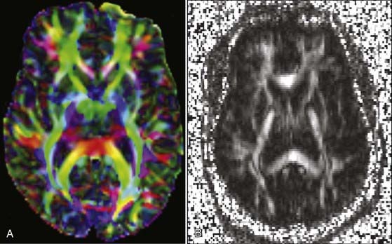
Once tensors have been calculated, they may be presented for interpretation in numerous ways. A mean diffusivity map portrays average molecular motion that is independent of tissue directionality, so voxels with high motion such as water will be bright and voxels with low motion such as gray matter will be dark. A fractional anisotropy (FA) map represents the colinearity and integrity of fibers, and therefore large tracts with parallel white matter bundles, as seen in the callosum fibers and descending corticospinal tract, appear white (FA approaches 1). CSF, gray matter, and crossing white matter tracts all lack parallel axonal configuration and thus appear dark or black (FA approaches 0). Color-encoded directional maps overlay fiber directional data on an FA image, with typical color assignments of red representing transverse fibers, green representing anteroposterior fibers, and blue representing superoinferior fibers; brighter or more saturated fibers indicate greater colinearity and hence greater anisotropy (Fig. 19-5).
Clinical Uses and Applications
DTI can be a very useful tool for demonstrating the integrity or compromise of tracts running between different areas of the brain. Four classic patterns of abnormal fiber orientation have been described: (1) deviated but otherwise preserved fiber tracts, (2) edematous tracts with diminished FA but preserved fiber tract orientation, (3) infiltrated tracts with diminished FA and abnormal fiber tract orientation, and (4) frank destruction of fiber tracts with negligible anisotropy.18 Figures 19-6 and 19-7 illustrate varieties of tract disruption.
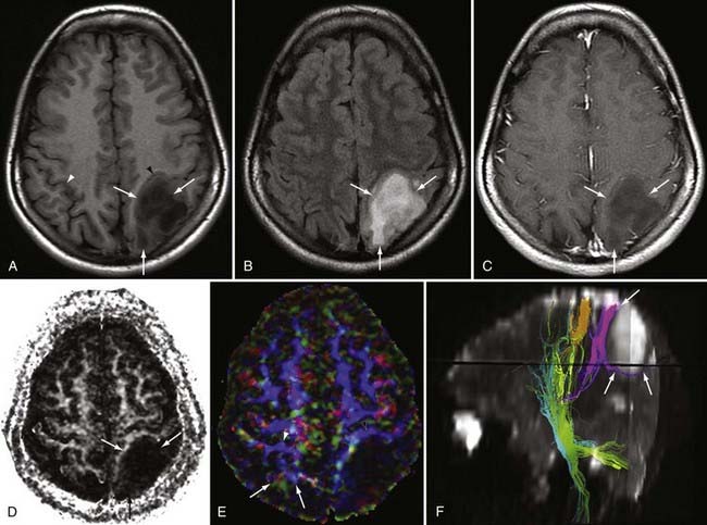
Such assessment of tracts can aid in planning treatment and determining prognosis, thereby allowing surgeons and radiation oncologists to protect tracts that are preserved while more aggressively addressing tracts that have already been destroyed. This has tremendous surgical importance because with these data a surgeon can maximize resection while minimizing risk to adjacent structures. A study by Kikuta and colleagues involving patients who had undergone resection for arteriovenous malformations (AVMs) found that incomplete tractography of the optic radiation was associated with visual field loss postoperatively.19 Such information not only assists in surgical planning but also helps prepare patients for potential outcomes of surgery. In addition, for patients undergoing surgery to treat brain tumors near the motor pathways, tractography may be used to identify initial sites for electrocortical stimulation, thus facilitating faster localization of eloquent cortex during surgery.
Applications of DTI extend beyond tumor evaluation. Preliminary studies suggest that DTI may be sufficiently sensitive to detect early changes in vulnerable regions in individuals with certain cognitive disorders, even at the presymptomatic or preclinical stages.20 Additional uses for tractography include assessment of patients with multiple sclerosis, and early studies in stroke patients suggest that DTI can aid in prognosis and may detect corticocortical rewiring.
DTI and tractography have recently been applied to the spinal cord, an area previously too degraded by artifact to image successfully. Some authors now suggest that FA data from DTI may be useful in distinguishing surrounding cord edema from tumor.21 In spinal cord AVMs, FA values in surrounding cord may improve after embolization and correlate with enhanced patient outcome.
Pitfalls and Limitations
A major limitation of conventional DTI is its poor distinction of crossing fiber tracts. When a voxel contains a homogeneous population of similarly oriented fibers, calculation of the dominant vector or water motion is straightforward. However, when a voxel contains crossing fibers, a simple tensor calculation is unable to reflect the more complex fiber configuration. In this instance, the major eigenvector may be calculated as the average of all voxel fibers, and as a result the eigenvector may not represent any of the dominant tracts.22 Newer techniques such as high–angular resolution diffusion imaging (HARDI) and Q-ball imaging may use 100 or more directions along with complex mathematical techniques to better characterize intravoxel tract ambiguity.23
Tractography depends on user input to define tracts of interest. Incorrect or suboptimal region-of-interest placement will result in misrepresented tracts. Mathematical assumptions will also influence tractography generation, with tract validity being dependent on appropriate definition of the maximal angulation within a voxel, the minimum FA value to tolerate while generating the tract, and the total path length. Because signal in the cord is more variable than signal in the brain and because the cord moves with CSF pulsation, spinal tractography proves considerably more challenging. In general, tractography in the cervical cord is easier to generate than in the thoracic cord, at least in part because of the greater pulsation effects in the mid and lower cord.21
Magnetic Resonance Angiography
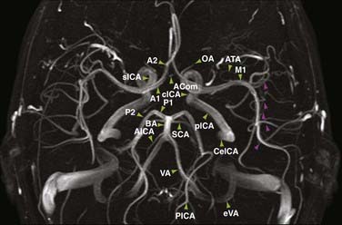
Evaluation of the intracranial vascular system is important in the diagnosis and planning of treatment of many vascular-related disease processes such as aneurysms, AVMs, infarction, and sinus venous thrombosis. Although the “gold standard” for evaluation of many vascular entities is currently digital subtraction angiography (DSA), magnetic resonance angiography (MRA) offers an alternative for the assessment of intracranial vessels that is both noninvasive and does not require the use of ionizing radiation. The three main varieties of MRA used clinically are time-of-flight (TOF), phase-contrast (PC), and contrast-enhanced (CE) techniques. Each MRA is typically postprocessed by a technologist before interpretation to yield maximum intensity projections that can be rotated in space for a three-dimensional (3D) effect (Fig. 19-8).
Physics
TOF MRA is performed by applying repetitive pulses to stationary tissues in a discrete volume of the brain, which results in saturation or suppression of signal in these tissues. Blood flowing into the volume has not been saturated and is therefore fully magnetized; this in-flowing blood therefore provides the only significant signal within the imaging slab. The intrinsic contrast that is derived from flowing blood eliminates the need for injection of contrast material to visualize the intracranial vessels. The pulse sequence used typically consists of a gradient recalled echo (GRE) sequence, which is acquired with either a two-dimensional (2D) or 3D technique. 2D TOF images are obtained as contiguous or slightly overlapped sections, whereas 3D TOF images are derived from one or more overlapping 3D volumes. Of these two methods, 3D TOF is more commonly used than 2D TOF because of its superior spatial resolution.24
In PC MRA, the vascular contrast is obtained by applying a bipolar phase-encoding gradient and a velocity-encoding (VEnc) factor.25,26 Phase shifts in moving spins or flowing blood are obtained when gradients with opposing polarities are applied twice during a single RF excitation. This method results in nulling of signal from stationary tissue while exploiting signal from flowing blood. Visualization of blood flow depends on the velocity of the flow. In specific encoding orientations, middle-gray usually represents no flow, whereas progressively increasing shades of white or black indicate directionally encoded higher velocities up to the predefined VEnc factor. Blood that flows at velocities higher than the VEnc factor will demonstrate aliasing, a situation in which signal intensity “wraps around” and will therefore be opposite that expected. In other words, if flow in a certain direction matches the VEnc factor, it will be encoded as white, but any greater velocity in that direction will actually appear as black. Because arterial flow is more rapid than venous flow, the typical arterial VEnc factor intracranially measures greater than 60 to 80 cm/sec, whereas slow flow within veins and venous sinuses is best imaged with a VEnc factor of 20 cm/sec or less.26 Images generated from this technique provide not only direction of flow but also magnitude of flow.
CE MRA uses a high-resolution T1-weighted technique in which the vessels are accentuated by a bolus of gadolinium chelate. The 2% to 3% concentration of gadolinium contrast agent in blood (by volume) causes a marked T1-shortening effect in vessels with a resultant increase in vessel signal. CE MRA provides anatomic information related to lumen diameter and the concentration of contrast material in vessels rather than physiologic information reflecting the flow rate, as calculated with TOF and PC techniques. Advantages of CE MRA over non-CE techniques include higher signal-to-noise ratios, decreased susceptibility to artifacts caused by pulsatility and flow, shorter image acquisition times, and temporal resolution that illustrates patterns of flow over time. Older CE MRA paradigms (e.g., elliptic-centric techniques) had collected full RF spectral data during the bolus, so only about three full-volume MRA repetitions could be acquired per minute. However, with that technique, the intended arterial-phase imaging was frequently obscured by venous enhancement. The need for improved temporal resolution led to the development of time-resolved CE MRA, such as TRICKS (time-resolved imaging of contrast kinetics) and TREAT (time-resolved echo-shared angiography technique).24 These sequences improve temporal resolution by repetitively acquiring the center of the RF spectrum along with varying peripheral portions during each acquisition; data missing from unsampled regions are interpolated by using data obtained at other points in time. This development enables more rapid 3D acquisitions before, during, and after transit of a contrast bolus, thereby allowing identification of the arterial, capillary, and venous phases.27,28
Clinical Uses and Applications
The angiographic modality with unparalleled spatial and temporal resolution is DSA. However, manipulation of catheters in the aorta or in the carotid or vertebral arteries, even by an experienced operator, is associated with a 1.3% risk for a cerebral event.29 Therefore, in clinical practice most institutions still use noninvasive techniques such as computed tomographic angiography (CTA) or MRA for preliminary evaluation of the vascular tree in the clinical setting of infarction, aneurysm, AVM, dural arteriovenous fistula (AVF), and veno-occlusive disease.
Stroke
A cerebrovascular accident, or stroke, is major cause of morbidity and mortality. It is the third most common cause of death in the United States, with approximately 795,000 cases occurring annually. The majority of these cases are caused by atherosclerotic disease, which results in stenosis and progressive occlusion of an arterial vessel. This can lead to ischemia and potential infarction of the brain tissue involved. MRA has been used to study the major arterial intracranial vessels to evaluate the effect of atherosclerotic disease. Specifically, 3D TOF MRA has been used as a screening method in stroke patients because it is minimally invasive and provides a reasonable assessment of the degree of vessel occlusion. Studies have shown 100% detection of vessel occlusion on 3D TOF MRA when correlated with DSA; however, grading of stenosis is less accurate (61%) when using MRA.30 Additionally, visualization of vessels that demonstrate slow or turbulent flow can be improved with the use of contrast material injected intravenously. For example, CE MRA has been shown to offer better visualization of the internal cerebral and middle cerebral arteries that exhibit artifactual narrowing on 3D TOF MRA because of slow or turbulent flow.31 Although such limitations exist, TOF MRA remains an important sequence for evaluation of the intracranial arterial circulation in patients with acute neurological symptoms.
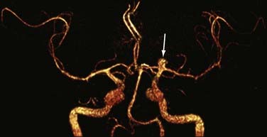
Intracranial Aneurysms
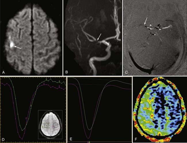
Detection of intracranial aneurysm can be done with noninvasive techniques such as MRA and CTA. 3D TOF MRA has been shown to have an overall sensitivity of 87% and specificity of 95% for the detection of intracranial aneurysms (Fig. 19-9). The sensitivity for detection of aneurysms larger than 3 mm is greater than that for aneurysms 3 mm or smaller (94% versus 38%) on older 1.5T scanners.32 At a magnetic field strength of 3T, aneurysms as small as 1 mm can be detected.33 Both TOF MRA and CE MRA are optimized to show vessel lumens; apical thrombus may remain undetected unless MRA is correlated with conventional sequences that are more sensitive for nonflowing blood.
Studies have shown similarities and differences between 3D TOF MRA and CE MRA in the detection of aneurysms. One study demonstrated no significant difference in the quality of the images and equal detection rates for both techniques.34 Another study showed that 3D TOF MRA detected more aneurysms than CE MRA did,35 whereas a third study indicated a sensitivity of 100% and a specificity of 94% for CE MRA, hence suggesting that CE MRA may be superior to the 3D TOF technique.36 Thus, there remains no clear consensus regarding which modality is superior, but both provide relatively accurate noninvasive methods for the detection of aneurysms.
MRA has also been studied for the follow-up of intracranial aneurysms treated by coil embolization. Serial studies have been performed with the use of both 3D TOF and CE MRA after treatment to evaluate for delayed aneurysm configuration because recanalization is estimated to occur in 10% to 40% of patients.37 Studies evaluating residual flow in coil-treated aneurysms have shown a sensitivity and specificity of 81% and 90.6%, respectively, for 3D TOF MRA and 86.8% and 91.9%, respectively, for CE MRA.38 It has been suggested that CE MRA may be slightly more sensitive in evaluating residual slow flow.24 DSA does remain the gold standard for evaluation of residual filling in treated aneurysm, but studies have shown 86% to 94% agreement between 3D TOF MRA evaluation and DSA.39–41
Vascular Malformations
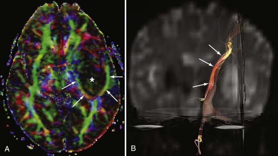
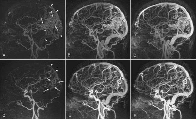
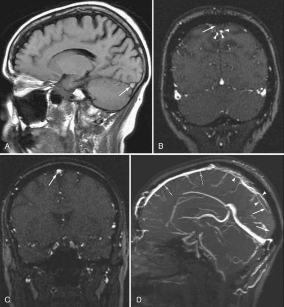
AVMs and AVFs are typically evaluated with DSA because of its excellent spatial and temporal resolution. However, MRA techniques may also provide an accurate noninvasive method for preoperative planning and evaluation of AVMs.42,43 3D TOF MRA and PC MRA allow characterization of flow in abnormal vessels, but they do not provide information on the hemodynamics of vascular malformations.44 Because definition of the architecture in and around malformations (e.g., arterial feeders, nidus size, and draining veins) is crucial in the evaluation of AVMs, advances in temporal resolution have had a large impact on noninvasive evaluation of these abnormalities. Indeed, ultrafast CE MRA and time-resolved CE MRA techniques have been shown to define relationships between lesions and the vasculature better than TOF and routine CE MRA techniques.45,46 Specific types of time-resolved CE MRA such as TRICKS MRA have been developed to provide hemodynamic information that gives one the ability to detect processes previously undetectable on noninvasive imaging, such as early venous drainage (Fig. 19-10).24 For example, in a small series of 40 patients, time-resolved MRA at 3 T was shown to be a reliable technique for the evaluation and surveillance of dural AVFs.47
Intracranial Venous System and Sinus Venous Thrombosis
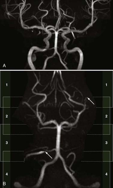
MRA techniques can be applied to study the intracranial venous system. Although arterial flow provides robust signal on 3D TOF sequences, the slower flow in veins provides more limited signal with 3D techniques. 2D TOF techniques are used instead because they offer excellent sensitivity for slow flow and less saturation effects than with 3D TOF techniques (Fig. 19-11).48 2D TOF best depicts flow perpendicular to the scanning plane, so areas of turbulent or tortuous flow (e.g., from the straight sinus through the transverse sinus through the sigmoid sinus) may require imaging in more than one acquisition plane to adequately represent flow patterns. In addition to TOF magnetic resonance venography (MRV), 2D or 3D PC MRV may be used because these techniques can indicate not only the rate of flow but also the directionality of flow. However, the dependence of PC MRV on operator-defined VEnc parameters may complicate its use,49 with incorrect assumptions at the time of scanning potentially leading to artifacts on the final images.
MRV can be enhanced by exploiting the paramagnetic effects of intravenous gadolinium. CE MRV has been shown to provide significantly better visibility of venous structures, including deep cerebral veins, than possible with the TOF technique. Selected venous structures studied in a small group of patients demonstrated visibility of 99% with CE MRV and 72% with TOF MRV. CE MRV can also be helpful in reducing the effects of turbulent flow on visualization of the venous sinuses.50
Pitfalls and Limitations
Spin dephasing can occur when blood flow is complex or turbulent and when vessels are in close proximity to tissues with short T1 properties, such as fat and subacute hemorrhage (methemoglobin). This configuration may result in loss of signal on TOF and PC MRA. Slow flow can also result in similar loss of signal on these imaging sequences because of spin saturation.51,52 Flow saturation effects can be diminished by using the “multiple overlapping thin slab acquisition” (MOTSA) technique for 3D TOF MRA (Fig. 19-12). Most institutions use three or four such slabs in an MRA acquisition through the head; this technique improves flow signal in vessels but lengthens imaging times.
Velocity aliasing can be seen with PC MRA when true velocities exceed the VEnc parameter of the imaging sequence.53 This may result in the perception of motion opposite the actual direction of blood flow; however, experienced radiologists will recognize the abrupt transition from black to white (or vice versa) as artifactual. In addition, factors such as lengthier acquisition times, lower spatial resolution, and artifacts related to pulsatile flow have limited the use of PC MRA in comparison to TOF and CE MRA.54 Thus, many sites reserve PC MRA to answer specific questions about flow directionality rather than including it as a standard imaging sequence.
Studies have reported high sensitivity and specificity ranging from 94% to 96% for 3D TOF MRA in the evaluation of intracranial stenosis. However, the MRA technique has a tendency to overestimate the degree of stenosis. A small study demonstrated overestimation of stenosis in 37% of diseased intracranial arterial segments with 3D TOF MRA when compared with DSA.55 Even though such measurement errors do limit the positive predictive value of TOF MRA in evaluating intracranial stenosis, this technique is still frequently used because of its high negative predictive value and its noninvasive technique.44
Failure to visualize appropriate signal in a normally flowing sinus may relate to MRV acquisition in a plane parallel to that of venous flow. This is a common limitation in the interpretation of these images and often mandates closer assessment of the source images. In instances in which true thrombosis is suspected, the acquisition plane may be modified, or CE MRV may be performed to improve sinus visualization.49
Phase-Contrast Magnetic Resonance Imaging of Cerebrospinal Fluid Flow
Physics
As in PC MRA, a PC acquisition can be used to quantify the rate and directionality of CSF flow. A similar bipolar gradient is applied to stationary tissue to cancel the magnetization from stationary spins and null the signal from these tissues. CSF that moves through the plane of acquisition between two separate gradient pulses will experience a net phase shift that is proportional to its velocity along a selected axis.56,57 The VEnc factors used in PC CSF studies are typically lower than those used for PC MRA, averaging 10 to 15 cm/sec. Imaging is usually acquired in the midline sagittal plane, although other orthogonal or oblique planes can be prescribed as well if needed.
PC CSF study differs from PC MRA in its use of cardiac gating. Hence, with this technique, magnitude and direction of flow can be segregated by phase in the cardiac cycle. Sixteen phases are typically acquired through the cardiac cycle, with triggering generally based on detection of each electrocardiographic R wave.58 In patients with normal sinus rhythm, adequate data are acquired through the cardiac cycle. Certain arrhythmias may compromise gating, however, and limit signal, particularly in the later phases.
Clinical Uses and Applications
PC MRI has been used to evaluate CSF flow in a wide range of cerebral disorders, including communicating hydrocephalus, normal-pressure hydrocephalus, and aqueductal stenosis. Recently, analysis of CSF pulsation in the axial plane at the foramen magnum has improved our understanding of the role of CSF flow disturbances in patients with symptomatic Chiari I malformations. PC MRI has been used to demonstrate elevated peak systolic velocities through the subarachnoid space and foramen magnum in these patients in comparison to normal subjects.59
Normal Cerebrospinal Fluid Flow
PC MRI sequences are usually analyzed in both static and cine formats. Typically, CSF flow sequences will generate magnitude, phase, and three orthogonal PC flow-encoded sets. Of greatest utility are the directional series that characterize flow within a structure. In the case of midline CSF flow from the third ventricle through the fourth ventricle outlet foramina, the most useful direction would conform most closely to the z-axis (Fig. 19-13). Shades representing one direction versus another may vary by scanner vendor; in practice, radiologists typically refer to the structures with known flow patterns (e.g., the deep venous system) to determine which shades represent which directions of flow.
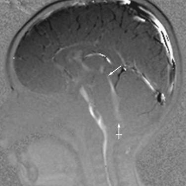
During a normal cardiac cycle, there is rhythmic movement of not only CSF but also brain parenchyma. Cardiac pulsations are transmitted through the intracranial arteries and capillaries and result in motion within the CSF. The relationship between the cardiac cycle and CSF is perceived as normal oscillatory CSF flow. During systole, expansion of the cerebral arterial vessels creates a pressure wave within the subarachnoid CSF. This pressure wave is transmitted through the intracranial subarachnoid space and results in outflow of CSF through the foramen magnum into the compliant spinal CSF space. In diastole, the arterial relaxation and resulting change in intracranial pressure cause CSF to flow back into the cranium through the foramen magnum.57,60 PC MRI techniques can be used to demonstrate the pulsatile flow within the CSF compartments and have been used to demonstrate the mechanical coupling between blood flow and CSF flow.61–64 Cine CSF flow studies have shown that normal CSF pulsations exhibit a timed sequence of oscillatory flow at specific sites in the ventricular system and subarachnoid spaces.58 The full length of the aqueduct can often be outlined by upward and downward waves of CSF pulsation (Fig. 19-14). CSF flow within the aqueduct is directed caudally during systole and cranially during diastole with an approximate flow velocity of 3 to 5 cm/sec.65

Abnormal Flow of Cerebrospinal Fluid
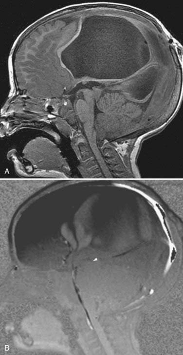
Alterations in normal CSF flow dynamics can be seen in a variety of neurological conditions. Normal oscillatory CSF can be affected when soft tissue impinges on or impacts the foramen magnum, as seen in symptomatic Chiari I malformations. Abnormal flow can also occur in patients with Dandy-Walker malformations, arachnoid cysts, or fourth ventricular outlet obstruction. CSF pulsation waves in these cases appear confined to the isolated space without detection of any significant CSF flow across the point of obstruction (Fig. 19-15).58 A mass that partially obstructs CSF outflow may also alter the time course of CSF pulsations.
An imbalance between intracranial blood and CSF flow has been suggested to be responsible for certain neurological disorders such as normal-pressure hydrocephalus.66 PC MRI has provided a means for the measurement of CSF flow at the aqueductal level. This has allowed improvement in diagnosis and management of patients with communicating hydrocephalus.67–69 It has been shown that a small group of symptomatic patients with CSF stroke volume greater than 42 µL per cycle may benefit from CSF shunting69; in normal volunteers the aqueductal stroke volume averages 39.51 ± 18.21 µL per cycle (range, 8.68 to 71.7).70 Quantification of the peak flow rate has likewise been suggested as an appropriate means for detecting abnormal aqueductal flow.71
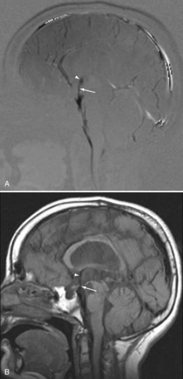
The use of PC MRI has also had important implications in the management of aqueductal stenosis or compression and the management of posterior third ventricle masses. The diagnosis of impaired flow through the aqueduct as the cause of hydrocephalus can direct management to endoscopic third ventriculostomy, which has shown success in the treatment of obstructive hydrocephalus.72,73 Although conventional MRI may demonstrate signs of aqueductal stenosis such as triventricular dilation or downward bulging of the third ventricle, evaluation with these signs alone is subjective and highly dependent on observer experience.74 PC MRI offers a reliable, reproducible, and accurate method for the diagnosis of aqueductal compromise in patients with suspected obstructive hydrocephalus by demonstrating absence of CSF flow (Fig. 19-16).75
Pitfalls and Limitations
The accuracy of CSF flow evaluation can be limited if the proper VEnc factor is not correctly selected by the operator. If CSF velocity exceeds the preselected VEnc parameter, aliasing or phase wraparound may occur. It is important to understand that the information acquired with PC MRI techniques without the use of true cardiac gating is an approximation of true CSF flow. The images obtained do not represent specific data points within the cardiac cycle but rather are approximations of preselected intervals with respect to the heart rate.58
Knowledge of certain pitfalls in PC MRI can greatly enhance diagnostic accuracy. For example, absent CSF pulsation may not indicate aqueductal obstruction; in some situations slow flow of CSF in general (as with obstruction at the level of the foramen of Monro by a colloid cyst) may result in reduced CSF flow downstream that could be interpreted as impaired flow through the aqueduct.63 In addition, CSF pulsations can appear to be discontinuous in a patent CSF space when there is converging flow, turbulence, or aliasing of pulsations.58
Perfusion-Weighted Imaging
Physics
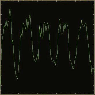
Dynamic susceptibility contrast perfusion-weighted imaging (PWI) exploits changes in T1 and T2 tissue contrast during a gadolinium bolus. For brain tumor imaging, a standard gadolinium dose (0.1 mmol/kg of body weight, typically corresponding to 15 to 20 mL of contrast agent) will provide an excellent signal-to-noise ratio with GRE EPI.76 Typical injection rates typically range from 2.5 to 5.0 mL/sec, and many sites use a double-barreled injector to flush saline after gadolinium to maintain a tight contrast bolus. The brain volume is scanned repeatedly before, during, and after the bolus, perfusion, and a time-intensity curve is generated for each voxel (Fig. 19-17). In general, the area under the curve correlates with CBV, the maximum slope of the curve roughly approximates CBF, and MTT refers to the width of the susceptibility curve. These three parameters are related by the equation CBF = CBV/MTT.77 It is worth noting that unlike CT perfusion, in which image density is linearly dependent on contrast concentration, in MR perfusion the relationship of signal to contrast concentration is curvilinear. As a result, most contrast MR perfusion studies in the brain will refer to relative CBV and relative CBF, and therefore comparison of suspected pathologic perfusion with normal contralateral perfusion is necessary.
A less prevalent variety of dynamic scanning is permeability imaging (Fig. 19-18). Although gadolinium does not normally pass through the blood-brain barrier (BBB), when the BBB is disrupted there is slow extravasation of contrast material into surrounding tissue. The pattern and rate of extravasation can be documented by dynamic repetitive acquisition of rapid T1-weighted MR images. This technique enables calculation of the microvascular permeability of the BBB. Permeability may be followed by perfusion imaging in one study session, with the added advantage that the permeability scan pre-enhances pathologic tissue and thus results in more normal return of the perfusion curve to baseline during PWI.
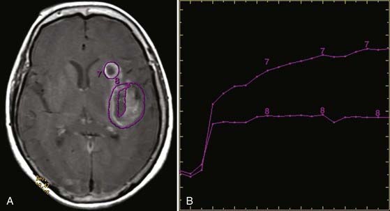
FIGURE 19-18 Permeability map in the same patient as in Figure 19-17. A, Axial T1-weighted gadolinium-enhanced image showing region-of-interest placement and (B) corresponding time-dependent enhancement curves. Curve 7 from the more anterior cavity shows a rapid first-phase rise and continued rise in the second phase at a lower rate. This is suggestive of radiation necrosis. Curve 8 from the necrotic cavity more posteriorly shows a rapid rise in the first phase but leveling out in the second phase. This is suggestive of viable tumor.
Arterial spin labeling (ASL) does not use intravenous gadolinium but instead assesses perfusion by labeling protons in the large arteries of the neck.78,79 These labeled protons then course intracranially within the blood pool and result in diminished signal. A second acquisition is generated without water labeling to serve as a baseline volume. Hemodynamic parameters and maps are generated on the basis of differences between the two acquisitions (Fig. 19-19).80
Clinical Uses and Applications
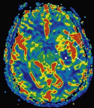
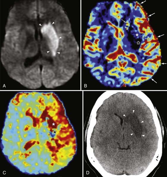
The combination of PWI and DWI in patients with brain ischemia can help distinguish viable tissue that is at risk for infarction (i.e., the penumbra) from the nonviable infarcted tissue core, which would have DWI restriction and markedly reduced CBV (Fig. 19-20).77 In addition to its application in cerebral ischemia from large-artery stenosis, as well as small-vessel disease, PWI can be used to characterize changes in perfusion in such entities as vasculitis, moyamoya, and vasospasm (Fig. 19-21). This holds particular promise in the assessment of peripheral ischemia in the setting of vasospasm (as from subarachnoid hemorrhage), which is difficult to quantify with catheter angiography.
Perfusion examinations are also frequently performed to estimate the hemodynamics of brain tumors. Perfusion data can aid in the differential diagnosis, with increased perfusion seen in gliomas as a result of angiogenesis related to aggressiveness and tumor viability.81 PWI has also become useful after treatment in distinguishing radiation necrosis from tumor recurrence.82 Both tumor growth and radiation necrosis will exhibit contrast enhancement related to disruption of the BBB, but the enhanced perfusion of neoplastic tissue (similar to or greater than adjacent “normal” tissue) contrasts with the diminished perfusion in radiation necrosis. Identification of zones of hyperperfusion may also help the surgeon target the most metabolically active area if the patient requires subsequent biopsy.83
Pitfalls and Limitations
With regard to tumors, distinction between tumor growth/recurrence and radiation necrosis can still be confusing and problematic, especially since both processes may coexist in similar areas.84 In addition, calculation of relative CBV can be grossly inaccurate in lesions such as glioblastoma multiforme, in which there is severe breakdown of the BBB.78 Furthermore, the extent of tumor infiltration into adjacent tissue is suboptimally characterized, particularly in areas where there is early infiltration but not yet neovascularity. Finally, tumor histology cannot reliably be inferred from perfusion data because some of the lower grade cerebral tumors such as oligodendrogliomas can have markedly increased perfusion that would otherwise be more suggestive of higher grade tumors.
Functional Magnetic Resonance Imaging
Physics
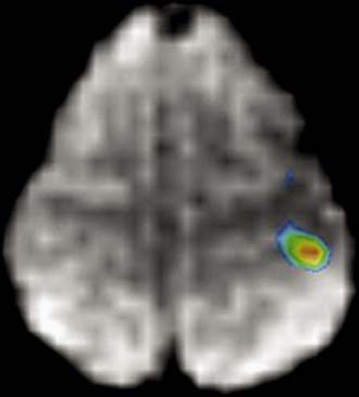
Functional MRI (fMRI) characterizes brain hemodynamic activity by indirectly revealing areas of neuronal activation after various stimulation by motor, visual, auditory, and tactile sensory input, most commonly in the form of “block paradigms.” Shortly after presentation of stimuli (or the onset of motor activity), the increase in cortical activity leads to increase in local CBF. The oxygen delivered by this increased blood flow is greater than the demand of tissue for oxygen, and as a result there is a net increase in oxyhemoglobin in the capillary bed. This increase in oxyhemoglobin is associated with a relative decrease in deoxyhemoglobin, whose paramagnetic properties ordinarily cause a reduction in local signal. Hence, with the reduction in deoxyhemoglobin comes a transient net increase in local signal.85 Because this technique depends on variation in oxygenation levels in blood, it is frequently referred to as BOLD imaging (Fig. 19-22).
BOLD EPI therefore identifies areas of increased MR signal from activated brain cortex. In practice, typical paradigms consist of three or four sets of alternating “on” periods, where sensory stimulation, cognitive tasks, or motor activity is present, and “off” periods, which are free of such stimulation. Differences between “on” and “off” measurements help determine where blood flow is affected by the stimulus or activity. Activation maps are generated by determining the statistical threshold above which true activity is likely. This activation pattern is then typically color-coded and superimposed on a high-resolution T1-weighted MRI sequence of the same section or on a 3D model for anatomic recognition.86
Clinical Uses and Applications
Mapping of cognitive functions has clear implications for surgical planning (Fig. 19-23). Preoperative identification may limit intraoperative awake testing if certain functions are localized away from the surgical bed. Functional data can be further exploited by processing in conjunction with DTI data; a site of activation can serve as a seed for DTI tractography to identify the trajectory of fibers (such as pyramidal tracts) that emanate from certain cortical areas so that they may be avoided during surgery.87
fMRI may also be used to demonstrate the eloquent regions of the brain and to determine right/left dominance. Most studies are sufficient to demonstrate the location of sensorimotor, speech, and auditory areas of the cerebral cortex.88
A growing research application of fMRI is for the elucidation of mechanisms of functional recovery from illness or brain injury. For example, in patients with motor deficits after stroke, fMRI may detect evidence of recruitment of brain regions or a shift in the activation center that may portend early stroke recovery.89
Pitfalls and Limitations
One must keep in mind that the BOLD technique indirectly measures neuronal activity based on oxygenation levels. Hence, some significant sites of neuronal activity may escape detection if they do not generate an adequate hemodynamic response. Furthermore, neuronal activation is markedly faster than the resulting hemodynamic response. Therefore, if used to detect epileptogenic foci, fMRI may better demonstrate secondary or propagated foci than the true or initial focus.90
Signal changes during BOLD imaging are dependent on magnetic field strength. It has been shown that activation of the primary motor and visual cortex at 3 T results in a 36% and 44% increase, respectively, in activation signal when compared to 1.5 T.91 This dramatic increase in signal-to-noise ratio may clarify true sites of activation at higher fields and may help in tasks that are traditionally difficult to image, such as in language paradigms and retinotopic mapping. However, with higher field strength comes greater susceptibility artifacts, so not all patients may benefit from scanning on a higher field system.
Patients with damage to certain cortical areas by tumors can produce false results. Thus for example, the regional hemodynamics about a brain tumor itself can produce areas of activation that are not truly related to the block paradigm stimuli.92 In addition, activation around tumors may be altered due to changes in vascular flow patterns, a phenomen known as neurovascular coupling.93
Proton Magnetic Resonance Spectroscopy
Physics
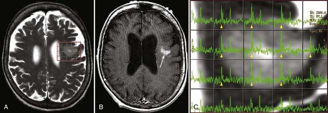
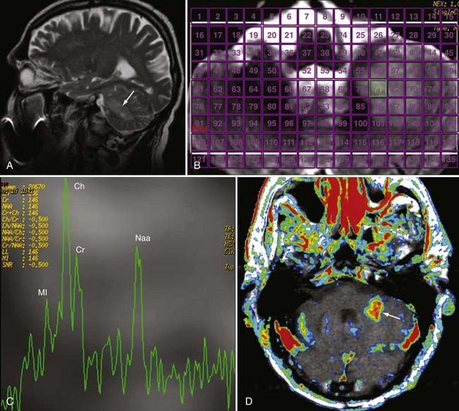
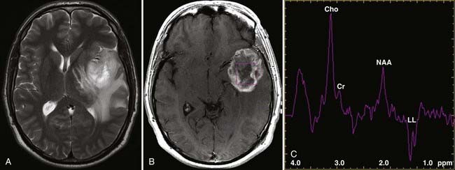
Proton magnetic resonance spectroscopy (1H-MRS, or simply MRS) is a noninvasive in vivo method of assessment of brain metabolites. MRS is based on “chemical shift,” or modification of proton resonance frequency, in certain molecular environments. Because the frequency of chemical shift varies by field strength, in clinical practice the shift is scaled to parts per million (ppm) so that peak locations are uniform across all varieties of scanners. The MRS data are ordinarily presented as a linear graph with the chemical shift (in ppm) on the x-axis and the plot of relative signal amplitude on the y-axis.94 However, metabolite-specific color gradients may also be superimposed over anatomic data to show relative quantities of these metabolites in specific areas.
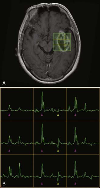
Two basic imaging methods are used, single voxel (SV) and multivoxel (MV, also called chemical shift imaging). In SV MRS, one discrete volume (voxel) of brain is chosen for the analysis, so the voxel must be placed precisely at the time of scanning for optimal results. MV MRS obtains the spectral data for a large grid of voxels simultaneously; this technique permits assessment of regional changes in metabolite concentrations, allows comparison of one voxel with another that is thought to be normal, and can help determine the most metabolically active zone to approach when a biopsy is being considered (Figs. 19-24 and 19-25).
Alanine (1.48 ppm) has a role in the citric acid cycle and can be increased in meningiomas.
Lipid (0.8 to 1.2 ppm) may be seen as a broad peak or two peaks at longer echo times, but it may be better visualized on MRS with short echo times. Lipid can be seen in areas of increased cell turnover, but its presence may also indicate voxel contamination by fat in the diploic space, the scalp, and subcutaneous tissues when the voxel is placed near one of these structures.94
Clinical Uses and Applications
MRS is now perhaps most widely used for the characterization of brain neoplasms (Fig. 19-26). In general, with increasing grade of glioma, one sees a reduction in the NAA peak and elevation of the choline peak (Fig. 19-27). The ultimate diagnosis is made by pathologic evaluation, but MRS can aid in determining the prognosis in some patients; for example, the percent change in the choline-NAA ratio has been shown to be useful for predicting progression of brain tumor in children. Overall, spectroscopy should be considered as a supplement to other imaging data in tumor analysis. Integration of spectroscopy data with perfusion data, enhancement pattern, and the remaining conventional MRI sequences increases the accuracy of predicting tumor grade and differentiating radiation necrosis from tumor recurrence.
In addition to tumors, recent work has shown the utility of MRS in other conditions. In seizure disorders, spectroscopy may be used to lateralize the side of hippocampal sclerosis by demonstrating decreased NAA and elevated Glx and myoinositol. It can also demonstrate bilateral temporal sclerosis, but correlation and confirmation with electroencephalography are advised.95 MRS may detect early changes in Alzheimer’s dementia before gross findings on MRI, with decreasing NAA and increasing myoinositol observed in the occipital, temporal, parietal, and frontal regions. In imaging of patients with traumatic brain injury, reductions in the NAA-creatine and NAA-choline ratios have been shown to be a reliable index for an unfavorable outcome and may help to identify which patients have a greater likelihood of regaining consciousness.96,97 Certain metabolic conditions have characteristic metabolite aberrations, such as the markedly elevated NAA in Canavan’s disease, which reflects a deficiency in the myelin synthesis pathway. In practice, MRS and DWI can be considered complementary methods for evaluating neurometabolic disease to give detailed information about the neurochemistry of affected brain areas.98
Pitfalls and Limitations
As stated earlier, the grade of an astrocytic tumor as a guide is thought to be proportional to the choline concentration. In evaluating the spectra of brain tumors, some highly malignant tumors such as glioblastoma multiforme may artifactually show low choline because of extensive necrosis. Furthermore, it is not uncommon to find some low-grade gliomas with very high choline-creatine and choline-NAA ratios. It is widely appreciated, however, that because of the heterogeneity of tumor, there is a significant overlap in the spectroscopy indices used to grade gliomas.99
Barnett A. Theory of Q-ball imaging redux: implications for fiber tracking. Magn Reson Med. 2009;62:910-923.
Barrett T, Brechbiel M, Bernardo M, et al. MRI of tumor angiogenesis. J Magn Reson Imaging. 2007;26:235-249.
Brandes AA, Tosoni A, Spagnolli F, et al. Disease progression or pseudoprogression after concomitant radiochemotherapy treatment: pitfalls in neurooncology. Neuro Oncol. 2008;10:361-367.
Cha S. Neuroimaging in neuro-oncology. Neurotherapeutics. 2009;6:465-477.
Detre JA. Clinical applicability of functional MRI. J Magn Reson Imaging. 2006;23:808-815.
Hattingen E, Blasel S, Dettmann E, et al. Perfusion-weighted MRI to evaluate cerebral autoregulation in aneurysmal subarachnoid haemorrhage. Neuroradiology. 2008;50:929-938.
Heiss WD, Sorensen AG. Advances in imaging. Stroke. 2009;40:e313-314.
Holdsworth SJ, Bammer R. Magnetic resonance imaging techniques: fMRI, DWI, and PWI. Semin Neurol. 2008;28:395-406.
Lacerda S, Law M. Magnetic resonance perfusion and permeability imaging in brain tumors. Neuroimaging Clin N Am. 2009;19:527-557.
Olivot JM, Marks MP. Magnetic resonance imaging in the evaluation of acute stroke. Top Magn Reson Imaging. 2008;19:225-230.
Ozsarlak O, Van Goethem JW, Maes M, et al. MR angiography of the intracranial vessels: technical aspects and clinical applications. Neuroradiology. 2004;46:955-972.
Paldino MJ, Barboriak DP. Fundamentals of quantitative dynamic contrast-enhanced MR imaging. Magn Reson Imaging Clin N Am. 2009;17:277-289.
Roberts TP, Mikulis D. Neuro MR: principles. J Magn Reson Imaging. 2007;26:823-837.
Soares DP, Law M. Magnetic resonance spectroscopy of the brain: review of metabolites and clinical applications. Clin Radiol. 2009;64:12-21.
Sunaert S. Presurgical planning for tumor resectioning. J Magn Reson Imaging. 2006;23:887-905.
Thurnher MM, Law M. Diffusion-weighted imaging, diffusion-tensor imaging, and fiber tractography of the spinal cord. Magn Reson Imaging Clin N Am. 2009;17:225-244.
Tieleman A, Deblaere K, Van Roost D, et al. Preoperative fMRI in tumour surgery. Eur Radiol. 2009;19:2523-2534.
Wallace RC, Karis JP, Partovi S, et al. Noninvasive imaging of treated cerebral aneurysms, part I: MR angiographic follow-up of coiled aneurysms. AJNR Am J Neuroradiol. 2007;28:1001-1008.
Wolf RL, Detre JA. Clinical neuroimaging using arterial spin-labeled perfusion magnetic resonance imaging. Neurotherapeutics. 2007;4:346-359.
Zou Z, Ma L, Cheng L, et al. Time-resolved contrast-enhanced MR angiography of intracranial lesions. J Magn Reson Imaging. 2008;27:692-699.
1 Sheerin F, Pretorius PM, Briley D, et al. Differential diagnosis of restricted diffusion confined to the cerebral cortex. Clin Radiol. 2008;63:1245-1253.
2 Le Bihan D. Molecular diffusion nuclear magnetic resonance imaging. Magn Reson Q. 1991;7:1-30.
3 Le Bihan D, Breton E, Lallemand D, et al. Separation of diffusion and perfusion in intravoxel incoherent motion MR imaging. Radiology. 1988;168:497-505.
4 Sener RN. Diffusion MRI: apparent diffusion coefficient (ADC) values in the normal brain and a classification of brain disorders based on ADC values. Comput Med Imaging Graph. 2001;25:299-326.
5 Schaefer PW, Grant PE, Gonzalez RG. Diffusion-weighted MR imaging of the brain. Radiology. 2000;217:331-345.
6 Sener RN. Diffusion MRI: apparent diffusion coefficient (ADC) values in the normal brain and a classification of brain disorders based on ADC values. Comput Med Imaging Graph. 2001;25:299-326.
7 Bastin ME, Delgado M, Whittle IR, et al. The use of diffusion tensor imaging in quantifying the effect of dexamethasone on brain tumours. Neuroreport. 1999;10:1385-1391.
8 Adams JH, Brierley JB, Connor RC, et al. The effects of systemic hypotension upon the human brain. Clinical and neuropathological observations in 11 cases. Brain. 1966;89:235-268.
9 Karaarslan E, Arslan A. Diffusion weighted MR imaging in non-infarct lesions of the brain. Eur J Radioly. 2008;65:402-416.
10 Moritani T, Shrier DA, Numaguchi Y, et al. Diffusion-weighted echo-planar MR imaging: clinical applications and pitfalls—a pictorial essay. Clin Imaging. 2000;24:181-192.
11 Erdogan C, Hakyemez B, Yildirim N, et al. Brain abscess and cystic brain tumor: discrimination with dynamic susceptibility contrast perfusion-weighted MRI. J Comput Assist Tomogr. 2005;29:663-667.
12 Stadnik TW, Demaerel P, Luypaert RR, et al. Imaging tutorial: differential diagnosis of bright lesions on diffusion-weighted MR images. Radiographics. 2003;23:e7.
13 Cole AJ. Status epilepticus and periictal imaging. Epilepsia. 2004;45(suppl 4):72-77.
14 Briellmann RS, Wellard RM, Jackson GD. Seizure-associated abnormalities in epilepsy: evidence from MR imaging. Epilepsia. 2005;46:760-766.
15 Castillo M, Mukherji SK. Diffusion-weighted imaging in the evaluation of intracranial lesions. Semin Ultrasound CT MR. 2000;21:405-416.
16 Holodny AI, Ollenschlager M. Diffusion imaging in brain tumors. Neuroimaging Clin N Am. 2002;12:107-124. x
17 Le Bihan D, Mangin JF, Poupon C, et al. Diffusion tensor imaging: concepts and applications. J Magn Reson Imaging. 2001;13:534-546.
18 Jellison BJ, Field AS, Medow J, et al. Diffusion tensor imaging of cerebral white matter: a pictorial review of physics, fiber tract anatomy, and tumor imaging patterns. AJNR Am J Neuroradiol. 2004;25:356-369.
19 Kikuta K, Takagi Y, Nozaki K, et al. Early experience with 3-T magnetic resonance tractography in the surgery of cerebral arteriovenous malformations in and around the visual pathway. Neurosurgery. 2006;58:331-337.
20 Ciccarelli O, Catani M, Johansen-Berg H, et al. Diffusion-based tractography in neurological disorders: concepts, applications, and future developments. Lancet Neurol. 2008;7:715-727.
21 Thurnher MM, Law M. Diffusion-weighted imaging, diffusion-tensor imaging, and fiber tractography of the spinal cord. Magn Reson Imaging Clin N Am. 2009;17:225-244.
22 Hagmann P, Jonasson L, Maeder P, et al. Understanding diffusion MR imaging techniques: from scalar diffusion-weighted imaging to diffusion tensor imaging and beyond. Radiographics. 2006;26(suppl 1):S205-S223.
23 Barnett A. Theory of Q-ball imaging redux: implications for fiber tracking. Magn Reson Med. 2009;62:910-923.
24 Huang BY, Castillo M. Neurovascular imaging at 1.5 tesla versus 3.0 tesla. Magn Reson Imaging Clin N Am. 2009;17:29-46.
25 Dumoulin CL, Cline HE, Souza SP, et al. Three-dimensional time-of-flight magnetic resonance angiography using spin saturation. Magn Reson Med. 1989;11:35-46.
26 Marks MP, Pelc NJ, Ross MR, et al. Determination of cerebral blood flow with a phase-contrast cine MR imaging technique: evaluation of normal subjects and patients with arteriovenous malformations. Radiology. 1992;182:467-476.
27 Carroll TJ, Korosec FR, Petermann GM, et al. Carotid bifurcation: evaluation of time-resolved three-dimensional contrast-enhanced MR angiography. Radiology. 2001;220:525-532.
28 Levy RA, Maki JH. Three-dimensional contrast-enhanced MR angiography of the extracranial carotid arteries: two techniques. AJNR Am J Neuroradiol. 1998;19:688-690.
29 Willinsky RA, Taylor SM, TerBrugge K, et al. Neurologic complications of cerebral angiography: prospective analysis of 2,899 procedures and review of the literature. Radiology. 2003;227:522-528.
30 Heiserman JE, Drayer BP, Keller PJ, et al. Intracranial vascular stenosis and occlusion: evaluation with three-dimensional time-of-flight MR angiography. Radiology. 1992;185:667-673.
31 Jung HW, Chang KH, Choi DS, et al. Contrast-enhanced MR angiography for the diagnosis of intracranial vascular disease: optimal dose of gadopentetate dimeglumine. AJR Am J Roentgenol. 1995;165:1251-1255.
32 White PM, Wardlaw JM, Easton V. Can noninvasive imaging accurately depict intracranial aneurysms? A systematic review. Radiology. 2000;217:361-370.
33 Tang PH, Hui F, Sitoh YY. Intracranial aneurysm detection with 3T magnetic resonance angiography. Ann Acad Med Singapore. 2007;36:388-393.
34 Nael K, Villablanca JP, Saleh R, et al. Contrast-enhanced MR angiography at 3T in the evaluation of intracranial aneurysms: a comparison with time-of-flight MR angiography. AJNR Am J Neuroradiol. 2006;27:2118-2121.
35 Gibbs GF, Huston J3rd, Bernstein MA, et al. 3.0-Tesla MR angiography of intracranial aneurysms: comparison of time-of-flight and contrast-enhanced techniques. J Magn Reson Imaging. 2005;21:97-102.
36 Metens T, Rio F, Baleriaux D, et al. Intracranial aneurysms: detection with gadolinium-enhanced dynamic three-dimensional MR angiography—initial results. Radiology. 2000;216:39-46.
37 Wallace RC, Karis JP, Partovi S, et al. Noninvasive imaging of treated cerebral aneurysms, part I: MR angiographic follow-up of coiled aneurysms. AJNR Am J Neuroradiol. 2007;28:1001-1008.
38 Kwee TC, Kwee RM. MR angiography in the follow-up of intracranial aneurysms treated with Guglielmi detachable coils: systematic review and meta-analysis. Neuroradiology. 2007;49:703-713.
39 Majoie CB, Sprengers ME, van Rooij WJ, et al. MR angiography at 3T versus digital subtraction angiography in the follow-up of intracranial aneurysms treated with detachable coils. AJNR Am J Neuroradiol. 2005;26:1349-1356.
40 Urbach H, Dorenbeck U, von Falkenhausen M, et al. Three-dimensional time-of-flight MR angiography at 3 T compared to digital subtraction angiography in the follow-up of ruptured and coiled intracranial aneurysms: a prospective study. Neuroradiology. 2008;50:383-389.
41 Buhk JH, Kallenberg K, Mohr A, et al. No advantage of time-of-flight magnetic resonance angiography at 3 tesla compared to 1.5 tesla in the follow-up after endovascular treatment of cerebral aneurysms. Neuroradiology. 2008;50:855-861.
42 Bednarz G, Downes B, Werner-Wasik M, et al. Combining stereotactic angiography and 3D time-of-flight magnetic resonance angiography in treatment planning for arteriovenous malformation radiosurgery. Int J Radiat Oncol Biol Phys. 2000;46:1149-1154.
43 Ehricke HH, Schad LR, Gademann G, et al. Use of MR angiography for stereotactic planning. J Comput Assist Tomogr. 1992;16:35-40.
44 Anzalone N. Contrast-enhanced MRA of intracranial vessels. Eur Radiol. 2005;15(suppl 5):E3-E10.
45 Duran M, Schoenberg SO, Yuh WT, et al. Cerebral arteriovenous malformations: morphologic evaluation by ultrashort 3D gadolinium-enhanced MR angiography. Eur Radiol. 2002;12:2957-2964.
46 Zou Z, Ma L, Cheng L, et al. Time-resolved contrast-enhanced MR angiography of intracranial lesions. J Magn Reson Imaging. 2008;27:692-699.
47 Farb RI, Agid R, Willinsky RA, et al. Cranial dural arteriovenous fistula: diagnosis and classification with time-resolved MR angiography at 3T. AJNR Am J Neuroradiol. 2009;30:1546-1551.
48 Liauw L, van Buchem MA, Spilt A, et al. MR angiography of the intracranial venous system. Radiology. 2000;214:678-682.
49 Leach JL, Fortuna RB, Jones BV, et al. Imaging of cerebral venous thrombosis: current techniques, spectrum of findings, and diagnostic pitfalls. Radiographics. 2006;26(suppl 1):S19-S41.
50 Farb RI, Scott JN, Willinsky RA, et al. Intracranial venous system: gadolinium-enhanced three-dimensional MR venography with auto-triggered elliptic centric-ordered sequence—initial experience. Radiology. 2003;226:203-209.
51 Bosmans H, Marchal G, Lukito G, et al. Time-of-flight MR angiography of the brain: comparison of acquisition techniques in healthy volunteers. AJR Am J Roentgenol. 1995;164:161-167.
52 Wilms G, Bosmans H, Demaerel P, et al. Magnetic resonance angiography of the intracranial vessels. Eur J Radiol. 2001;38:10-18.
53 Ozsarlak O, Van Goethem JW, Maes M, et al. MR angiography of the intracranial vessels: technical aspects and clinical applications. Neuroradiology. 2004;46:955-972.
54 DeLano MC, DeMarco JK. 3.0 T versus 1.5 T MR angiography of the head and neck. Neuroimaging Clin N Am. 2006;16:321-341. xi
55 Sadikin C, Teng MM, Chen TY, et al. The current role of 1.5T non-contrast 3D time-of-flight magnetic resonance angiography to detect intracranial steno-occlusive disease. J Formos Med Assoc. 2007;106:691-699.
56 Spilt A, Box FM, van der Geest RJ, et al. Reproducibility of total cerebral blood flow measurements using phase contrast magnetic resonance imaging. J Magn Reson Imaging. 2002;16:1-5.
57 Stivaros SM, Jackson A. Changing concepts of cerebrospinal fluid hydrodynamics: role of phase-contrast magnetic resonance imaging and implications for cerebral microvascular disease. Neurotherapeutics. 2007;4:511-522.
58 Naidich TP, Altman NR, Gonzalez-Arias SM. Phase contrast cine magnetic resonance imaging: normal cerebrospinal fluid oscillation and applications to hydrocephalus. Neurosurg Clin N Am. 1993;4:677-705.
59 Haughton VM, Korosec FR, Medow JE, et al. Peak systolic and diastolic CSF velocity in the foramen magnum in adult patients with Chiari I malformations and in normal control participants. AJNR Am J Neuroradiol. 2003;24:169-176.
60 Greitz D, Wirestam R, Franck A, et al. Pulsatile brain movement and associated hydrodynamics studied by magnetic resonance phase imaging. The Monro-Kellie doctrine revisited. Neuroradiology. 1992;34:370-380.
61 Levy LM, Di Chiro G. MR phase imaging and cerebrospinal fluid flow in the head and spine. Neuroradiology. 1990;32:399-406.
62 Quencer RM. Intracranial CSF flow in pediatric hydrocephalus: evaluation with cine-MR imaging. AJNR Am J Neuroradiol. 1992;13:601-608.
63 Quencer RM, Post MJ, Hinks RS. Cine MR in the evaluation of normal and abnormal CSF flow: intracranial and intraspinal studies. Neuroradiology. 1990;32:371-391.
64 Baledent O, Henry-Feugeas MC, Idy-Peretti I. Cerebrospinal fluid dynamics and relation with blood flow: a magnetic resonance study with semiautomated cerebrospinal fluid segmentation. Invest Radiol. 2001;36:368-377.
65 Mascalchi M, Ciraolo L, Tanfani G, et al. Cardiac-gated phase MR imaging of aqueductal CSF flow. J Comput Assist Tomogr. 1988;12:923-926.
66 Greitz D. The hydrodynamic hypothesis versus the bulk flow hypothesis. Neurosurg Rev. 2004;27:299-300.
67 Baledent O, Gondry-Jouet C, Stoquart-Elsankari S, et al. Value of phase contrast magnetic resonance imaging for investigation of cerebral hydrodynamics. J Neuroradiol. 2006;33:292-303.
68 Bradley WGJr. MR prediction of shunt response in NPH: CSF morphology versus physiology. AJNR Am J Neuroradiol. 1998;19:1285-1286.
69 Bradley WGJr, Scalzo D, Queralt J, et al. Normal-pressure hydrocephalus: evaluation with cerebrospinal fluid flow measurements at MR imaging. Radiology. 1996;198:523-529.
70 Florez N, Marti-Bonmati L, Forner J, et al. [Normal values for cerebrospinal fluid flow dynamics in the aqueduct of Sylvius through optimized analysis of phase-contrast MR images.]. Radiologia. 2009;51:38-44.
71 Gideon P, Sorensen PS, Thomsen C, et al. Assessment of CSF dynamics and venous flow in the superior sagittal sinus by MRI in idiopathic intracranial hypertension: a preliminary study. Neuroradiology. 1994;36:350-354.
72 Foroutan M, Mafee MF, Dujovny M. Third ventriculostomy, phase-contrast cine MRI and endoscopic techniques. Neurol Res. 1998;20:443-448.
73 Kim SK, Wang KC, Cho BK. Surgical outcome of pediatric hydrocephalus treated by endoscopic III ventriculostomy: prognostic factors and interpretation of postoperative neuroimaging. Childs Nerv Syst. 2000;16:161-168.
74 Kehler U, Regelsberger J, Gliemroth J, et al. Outcome prediction of third ventriculostomy: a proposed hydrocephalus grading system. Minim Invasive Neurosurg. 2006;49:238-243.
75 Stoquart-El Sankari S, Lehmann P, Gondry-Jouet C, et al. Phase-contrast MR imaging support for the diagnosis of aqueductal stenosis. AJNR Am J Neuroradiol. 2009;30:209-214.
76 Lacerda S, Law M. Magnetic resonance perfusion and permeability imaging in brain tumors. Neuroimaging Clin N Am. 2009;19:527-557.
77 Harris AD, Coutts SB, Frayne R. Diffusion and perfusion MR imaging of acute ischemic stroke. Magn Reson Imaging Clin N Am. 2009;17:291-313.
78 Heiss WD, Sorensen AG. Advances in imaging. Stroke. 2009;40:e313-e314.
79 Petersen ET, Zimine I, Ho YC, et al. Non-invasive measurement of perfusion: a critical review of arterial spin labelling techniques. Br J Radiol. 2006;79:688-701.
80 Paiva FF, Tannus A, Silva AC. Measurement of cerebral perfusion territories using arterial spin labelling. NMR Biomed. 2007;20:633-642.
81 Mechtler L. Neuroimaging in neuro-oncology. Neurol Clin. 2009;27:171-201. ix
82 Cha S, Knopp EA, Johnson G, et al. Intracranial mass lesions: dynamic contrast-enhanced susceptibility-weighted echo-planar perfusion MR imaging. Radiology. 2002;223:11-29.
83 Weber MA, Giesel FL, Stieltjes B. MRI for identification of progression in brain tumors: from morphology to function. Expert Rev Neurother. 2008;8:1507-1525.
84 Brandes AA, Tosoni A, Spagnolli F, et al. Disease progression or pseudoprogression after concomitant radiochemotherapy treatment: pitfalls in neurooncology. Neuro Oncol. 2008;10:361-367.
85 Roberts TP, Mikulis D. Neuro MR: principles. J Magn Reson Imaging. 2007;26:823-837.
86 Ramsey NF, Hoogduin H, Jansma JM. Functional MRI experiments: acquisition, analysis and interpretation of data. Eur Neuropsychopharmacol. 2002;12:517-526.
87 Sunaert S. Presurgical planning for tumor resectioning. J Magn Reson Imaging. 2006;23:887-905.
88 Blatow M, Nennig E, Durst A, et al. fMRI reflects functional connectivity of human somatosensory cortex. Neuroimage. 2007;37:927-936.
89 Detre JA. Clinical applicability of functional MRI. J Magn Reson Imaging. 2006;23:808-815.
90 Pouratian N, Sheth S, Bookheimer SY, et al. Applications and limitations of perfusion-dependent functional brain mapping for neurosurgical guidance. Neurosurg Focus. 2003;15(1):E2.
91 Kruger G, Kastrup A, Glover GH. Neuroimaging at 1.5 T and 3.0 T: comparison of oxygenation-sensitive magnetic resonance imaging. Magn Reson Med. 2001;45:595-604.
92 Tieleman A, Deblaere K, Van Roost D, et al. Preoperative fMRI in tumour surgery. Eur Radiol. 2009;19:2523-2534.
93 Ulmer JL, Kroower HG, Mueller WM, et al. Pseudo-reorganization of language cortical function at fme imaging: a consequence of tumor-induced neurovascular uncoupling. AJNR Am J Neuroradiol. 2003;24:213-217.
94 Soares DP, Law M. Magnetic resonance spectroscopy of the brain: review of metabolites and clinical applications. Clin Radiol. 2009;64:12-21.
95 Simister RJ, McLean MA, Barker GJ, et al. Proton MR spectroscopy of metabolite concentrations in temporal lobe epilepsy and effect of temporal lobe resection. Epilepsy Res. 2009;83:168-176.
96 Tshibanda L, Vanhaudenhuyse A, Boly M, et al. Neuroimaging after coma. Neuroradiology. 2010;52:15-24.
97 Ricci R, Barbarella G, Musi P, et al. Localised proton MR spectroscopy of brain metabolism changes in vegetative patients. Neuroradiology. 1997;39:313-319.
98 Cakmakci H, Pekcevik Y, Yis U, et al. Diagnostic value of proton MR spectroscopy and diffusion-weighted MR imaging in childhood inherited neurometabolic brain diseases and review of the literature. Eur J Radiol.. 2010;74:e161-e171.
99 Moller-Hartmann W, Herminghaus S, Krings T, et al. Clinical application of proton magnetic resonance spectroscopy in the diagnosis of intracranial mass lesions. Neuroradiology. 2002;44:371-381.