Pharmaceutical preformulation
Simon Gaisford
Chapter contents
Determination of melting point and enthalpy of fusion using differential scanning calorimetry
Solubility as a function of temperature
Measurement of intrinsic solubility
Selection of a salt-forming acid or base
Key points
• Preformulation is the stage in drug and dosage form development before formulation proper.
• Preformulation aims to optimize the process of turning a drug candidate into a drug product.
• During preformulation, the physicochemical properties of drug candidates are determined.
• Compaction requires good compression and cohesion properties.
The concept of preformulation
Formulation is the process of developing a drug candidate into a drug product. Initially, there may be a number of potential drug candidate molecules, each with a unique set of physicochemical properties and each showing activity towards a particular biological target. Ultimately, only one (at best) will be developed into a drug product. The decision to select a successful drug candidate to be developed does not depend on pharmacological efficacy alone. In practice, the physicochemical properties of the molecule affect how a material will process pharmaceutically, its stability, its interaction with excipients, how it will transfer to solution and, ultimately, will determine its bioavailability. It follows that characterizing the physicochemical properties of drug candidates early in the development process will provide the fundamental knowledge base upon which candidate selection, and ultimately dosage form design, can be made, reducing development time and costs.
It is an obvious point – but crucial to the task ahead – that usually nothing will be known about the physicochemical properties of a new drug candidate and these facts must be ascertained by a combination of scientific consideration of the molecular structure and experimentation. At this stage of the development, the new drug candidate is often somewhat impure and in very short supply. Normal formulation studies have to be modified to deal with this scenario.
Physicochemical properties can be split into those that are intrinsic to the molecule and those that are derived from bulk behaviour (e.g. of the powder or crystals). Intrinsic properties are inherent to the molecule and so can only be altered by chemical modification, while derived properties are the result of intermolecular interactions and so can be affected by solid-state form, physical shape and environment among other factors.
Determination of these properties for a new chemical entity is termed preformulation (literally the stage that must be undertaken before formulation-proper can begin).
Assay development
No relevant physicochemical property can be measured without an assay and so development of a suitable assay is the first step of preformulation. The first assay procedures should require minimal amounts of sample (since as little as 50 mg may actually exist of each compound). Ideally, experiments should allow determination of multiple parameters. For instance, a saturated solution prepared to determine aqueous solubility may subsequently be re-used to determine a partition coefficient.
Note that at this stage the determination of approximate values is acceptable in order to make a ‘go/no go’ decision in respect of a particular drug candidate, and so assays do not need to be as rigorously validated as they do later in formulation development. Table 23.1 lists a range of properties to be measured during preformulation, in chronological order, and the assays that may be used to quantify them. These properties are a function of molecular structure. Once known, further macroscopic (or bulk) properties of the drug candidate can be measured, Table 23.2. These properties result from intermolecular interactions. Note also that determination of chemical structure does not appear, as it is assumed the chemists preparing the candidate molecules would provide this information. Note also that solubility will be dependent upon physical form (polymorph, pseudo-polymorph or amorphous).
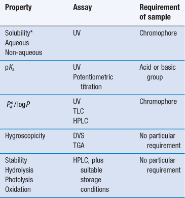
Table 23.2
Macroscopic (bulk) properties and the techniques used to determine them
| Derived property | Technique |
| Melting point | DSC or melting point apparatus |
| Enthalpy of fusion (and so ideal solubility) | DSC |
| Physical forms (polymorphs, pseudo-polymorphs or amorphous) | DSC, XRPD, microscopy |
| Particle shape Size distribution Morphology Rugosity Habit |
Microscopy Particle sizing BET (surface area) |
| Density Bulk Tapped True |
Tapping densitometer |
| Flow | Angle of repose |
| Compressibility | Carr’s index Hausner ratio |
| Excipient compatibility | HPLC, DSC |
The full characterization of a drug candidate (in the context of preformulation) should be possible with just ultraviolet (UV) spectroscopy, high-performance liquid chromatography (HPLC), differential scanning calorimetry (DSC), dynamic vapour sorption (DVS) and X-ray powder diffraction (XRPD). This explains the popularity of these techniques in pharmaceutical development. Thin-layer chromatography (TLC) and thermogravimetric analysis (TGA) provide useful supporting data, but neither is essential during the early stages.
Solubility
Aqueous solubility is a critical attribute. No drug will reach its ultimate therapeutic target without first being in solution. Consequently, it is the first physicochemical parameter to be determined. It has been estimated that, historically, up to 40% of drug candidates have been abandoned because of poor aqueous solubility, and between 35–40% of compounds currently in development have an aqueous solubility below 5 mg mL−1 at pH 7. The USP and PhEur provide definitions of solubility based on concentration (see Chapter 2 and in particular, Table 2.2).
Early determination of solubility gives a good indicator as to the ease of formulation of a drug candidate. Initial formulations, used for obtaining toxicity and bioavailability data in animal models, will need to be liquids for oral gavage or intravenous delivery, and a solubility above 1 mg mL−1 is usually acceptable. For the final product, assuming oral delivery in a solid form, solubility of the molecule above 10 mg mL−1 is preferable. If the solubility of the drug candidate is less than 1 mg mL−1 then salt formation, if possible, is indicated. Where solubility cannot be manipulated through salt formation, then a novel dosage form will be required.
Dissolution is a phase transition and in order to progress, solid-solid bonds must be broken (effectively, the solid melts), while solvent-solvent bonds must be broken and replaced by solute-solvent bonds (the drug molecules become solvated) (Chapter 2). With excess solid present, a position of equilibrium will be established between the solid and dissolved drug.
The concentration of drug dissolved at this point is known as the equilibrium solubility (usually referred to simply as solubility) and the solution is saturated. If the drug has an ionizable group then the equilibrium solubility of the unionized form is called the intrinsic solubility (So). This is important, because ionizable drugs will dissociate to a greater or lesser extent, influenced by solution pH, and this will affect the observed solubility.
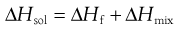
From a thermodynamic perspective, the energy input required to break the solid-solid bonds must equal the enthalpy of fusion (ΔHf) required to melt the solid (since the same bonds are broken). Unlike melting, however, in the case of dissolution there is an additional enthalpy change because solvent-solvent bonds are broken and solute-solvent bonds are formed (shown diagrammatically in Fig.2.2). The energy involved in this process is known as the enthalpy of mixing (ΔHmix). The net enthalpy of dissolution (ΔHsol) is thus the sum of the enthalpy of fusion and the enthalpy of mixing:
 (23.1)
Knowledge of this relationship between solubility and bond energy can be used during preformulation to make predictions of solubility from thermal energy changes (e.g. during melting and other phase changes).
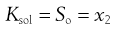
Thus, dissolution in the presence of a solid results in an equilibrium between the solid and the dissolved state. The equilibrium constant (Ksol) for the overall process of dissolution can be represented as:
 (23.2)
where a denotes the activity of the drug in solution aaq and in the solid phase as. Since the activity of a solid is defined as unity and in dilute solution activity approximates to concentration (solubility in this case) then:
 (23.3)
where So is again the intrinsic solubility and x2 denotes the saturated concentration of drug in mole fraction units (x1 being the mole fraction of the solvent).
It is possible to see from Equation 23.1 that the crystal lattice energy might affect solubility. There will also be an effect of temperature on solubility, since the position of the equilibrium between solid and dissolved drug will change. Both of these effects can be explored further through the concept of ideal solubility.
Ideal solubility
In the special case where the energy of the solute-solvent bond is equal to the energy of the solvent-solvent bond, then solute-solvent bonds may form with no change in intermolecular energy (i.e. ΔHmix = 0) and dissolution is said to be ideal. Ideal dissolution (although unlikely in reality) leads to ideal solubility and is an interesting theoretical position because it can be described in thermodynamic terms that allow calculation of the dependence of solubility with temperature.
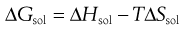
From Equation 23.1, if ΔHmix = 0 then ΔHf is equal to ΔHsol. Incidentally, since ΔHf must be positive (i.e. endothermic) ΔHsol must also be positive for ideal dissolution. For a process to occur spontaneously the Gibbs free energy (ΔG) must be negative. The familiar thermodynamic relationship for dissolution is:
 (23.4)
where T is temperature. ΔGsol is most likely to be negative when ΔHsol is negative but, as noted above, ΔHsol is frequently positive for dissolution. This means that for dissolution to occur spontaneously, the driving force must be an increase in entropy.
Equation 23.3 shows that solubility has the attributes of an equilibrium constant. This being so, it is possible to apply the van’t Hoff equation (Eqn 23.9), yielding:
 (23.5)
Making the assumption that ΔHf is independent of temperature, then integrating Equation 23.5 from Tm to T results in:
 (23.6)
where Tm is the melting temperature of the pure drug and T is the experimental temperature.
Equation 23.6 is very useful in preformulation, since it allows prediction of ideal solubility at a particular temperature if the melting temperature and enthalpy of fusion of the pure drug are known. This is why determination of melting point and enthalpy of fusion are the next physicochemical parameters to be determined during preformulation.
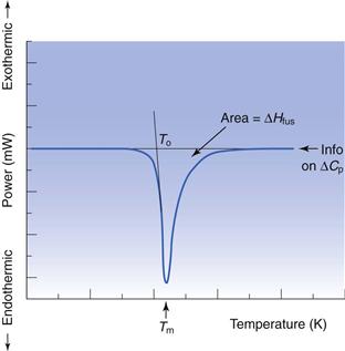
Determination of melting point and enthalpy of fusion using differential scanning calorimetry
The energy changes discussed above can be measured by differential scanning calorimetry (DSC). In DSC, the power required to heat a sample in accordance with a user-defined temperature program is recorded, relative to an inert reference. The heating rate (β) can be linear or modulated by a mathematical function. When the sample melts, energy will be absorbed during the phase change and an endothermic peak will be seen, Figure 23.1. The enthalpy of fusion is equal to the area under the melting endotherm while the melting temperature may be determined either as an extrapolated onset (To) or the peak maximum (Tm).
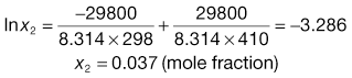
Box 23.1 Worked example
The melting temperature of aspirin is 137 °C and its enthalpy of fusion at the melting temperature is 29.80 kJ mol−1. What is the ideal solubility of aspirin at 25 °C?
Applying Equation 23.6:
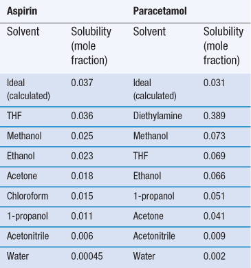
Invariably, real solutions do not show ideal behaviour because the assumptions made earlier that ΔHmix = 0 and that ΔHf is independent of temperature are not always valid. A negative (exothermic) enthalpy of mixing increases solubility, while a positive (endothermic) enthalpy of mixing reduces solubility. Table 23.3 lists the experimentally measured solubilities for aspirin and paracetamol in a range of solvents. Note that solubility in water is by far the lowest of any of the solvents shown, while solubilities in tetrahydrofuran (THF) and methanol approach ideality in the case of aspirin, and exceed ideality in the case of paracetamol.
The reason that so many solvents, and water in particular, display such non-ideal behaviour is because of significant intermolecular bonding resulting from their chemical structure and properties. The three primary chemical properties are the dipole moment, dielectric constant and capacity for forming hydrogen bonds.
A molecule has a dipole when there is a localized net positive charge in one part of the molecule and a localized net negative charge in another. Such molecules are said to be polar. Water is an example of a polar molecule. Drugs that have dipoles or dipolar character are generally more soluble in polar solvents.
Dielectric properties are related to the capacity of a molecule to store a charge and are quantified by a dielectric constant. Polar solvents may induce a dipole in a dissolved solute, which will increase solubility. The dielectric constants of a number of commonly used pharmaceutical solvents are given in Table 23.4. It can be seen that water has a high dielectric constant (78.5) relative to that of methanol (31.5) even though both are considered to be polar solvents.
Table 23.4
Dielectric constants of some common pharmaceutical solvents at 25 °C
| Solvent | Dielectric constant (no units, dimensionless) |
| Water | 78.5 |
| Glycerin | 40.1 |
| Methanol | 31.5 |
| Ethanol | 24.3 |
| Acetone | 19.1 |
| Benzyl alcohol | 13.1 |
| Phenol | 9.7 |
| Ether | 4.3 |
| Ethyl acetate | 3.0 |
Hydrogen bonding occurs when electronegative atoms (such as oxygen) come into close proximity with hydrogen atoms; electrons are pulled towards the electronegative atom creating a reasonably strong force of interaction. A drug that has a functional group capable of hydrogen bonding with water (such as —OH, —NH or —SH) should have increased aqueous solubility.
Solubility as a function of temperature
Equation 23.6 indicates that the heat of fusion should be determinable by experimentally measuring the solubility of a drug at a number oftemperatures (since a plot of lnx2 versus  should be linear and have a slope of
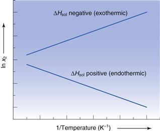
  ). Since ΔHfmust be positive, Equation 23.6 suggests that the solubility of a drug should increase with an increase in temperature. Generally, this agrees with everyday experience, but there are some drugs for which solubility decreases with increasing temperature. This is because an assumption was made in deriving Equation 23.6, namely that ΔHf was equal to ΔHsol. However, as noted above and as demonstrated by the data in Table 23.3, ΔHmix is frequently not zero. In cases where ΔHsol is negative (i.e. the heat of solution is exothermic), solubility will decrease with increasing temperature. These effects are shown in Figure 23.2.
Examples of data from three drug molecules plotted this way are given in Figure 23.3. While such plots are frequently found to be linear, they are usually plotted over a very narrow temperature range and the heat of fusion so calculated is rarely ideal, although it can be considered to be an approximate heat of solution.
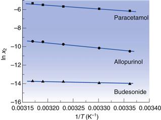
 for three drugs in water.
 Solubility and physical form
If molecules in the solid state are able to align in different patterns (the phenomenon of polymorphism, Chapter 8), then it is highly likely that the strength of the intermolecular bonds, and hence crystal lattice energy, will vary. Two polymorphs of the same drug will thus have different melting temperatures and heats of fusion. Usually the stable polymorph has the highest melting point and greatest heat of fusion and so, from Equation 23.6, the lowest solubility. Any metastable forms will, by definition, have lower melting points, lower enthalpies of fusion and so greater solubilities. The amorphous form, by virtue of not possessing a melting point, will have the greatest solubility. It is therefore clear that the solid-state structure of a new drug candidate should be determined during preformulation.
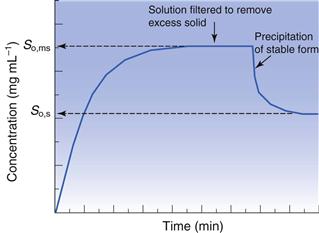
As discussed above, solubility is defined as the equilibrium between dissolved solute and the solid form. Thus, if a saturated solution is prepared by dissolving a metastable form and the excess solid is removed by filtration, the solution will be supersaturated with respect to the stable form. Ultimately, the stable form will precipitate as the system re-establishes a position of equilibrium (Fig. 23.4). Formulating any drug in a (solid) metastable form thus involves an element of risk; the risk being that the stable form will appear during storage or post-dissolution. In either case solubility will be reduced with, potentially, a consequential reduction in bioavailability.
Measurement of intrinsic solubility
Initially, during preformulation, solubility should be determined in 0.1 M HCl, 0.1 M NaOH and water. These ‘unsophisticated’ choices are determined by the scarcity of material at this stage. Saturated solutions can be prepared by adding an excess of solid to a small volume of solvent, agitating with time and then filtering.
Ultraviolet (UV) spectroscopy is the first choice assay, for reasons of familiarity, cost, the small volume of solution needed and the fact that the majority of drugs contain at least one functional group that absorbs in the UV region (190–390 nm). Table 23.5 lists the UV absorbance maxima for a series of common functional groups (called chromophores).
Table 23.5
UV absorbance maxima for a range of common functional groups
| Chromophore | λmax (nm) | Molar extinction (ε) |
| Benzene | 184 | 46700 |
| Naphthalene | 220 | 112000 |
| Anthracene | 252 | 199000 |
| Pyridine | 174 | 80000 |
| Quinoline | 227 | 37000 |
| Ethlyene | 190 | 8000 |
| Acetylide | 175–180 | 6000 |
| Ketone | 195 | 1000 |
| Nitroso | 302 | 100 |
| Amino | 195 | 2800 |
| Thiol | 195 | 1400 |
| Halide | 208 | 300 |
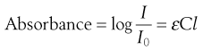
Excitation of the solute with the appropriate wavelength of light will reduce the amount of light passing through the solution. If the original light intensity is I0 and the amount of light passing through the sample (the transmitted light) is I, then the amount of light absorbed will be a function of the concentration of the solute (C) and the depth of the solution through which the light is passing (the path length, l). This relationship is usually expressed as the Beer-Lambert equation:
 (23.7)
where ε is a constant of proportionality called the ‘molar extinction coefficient’.
Higher values of ε mean greater UV absorbance by the solute. Values of ε for a range of functional groups are given in Table 23.5; it can be seen that groups containing large numbers of delocalized electrons, such as those containing benzene rings, have much greater ε values that groups containing simple carbon-carbon double bonds. The absorbance of a chromophore can be affected by the presence of an adjacent functional group if that group has unshared electrons (an auxochrome). A list of common auxochromes and their effects on the molar extinction coefficients of their parent benzene ring is given in Table 23.6.
Table 23.6
The effect of auxochromes on the UV absorbance of the parent compound C6H5-R
| Substituent | λmax (nm) | Molar extinction (ε) |
| —H | 203.5 | 7400 |
| —CH3 | 206.5 | 7000 |
| —Cl | 209.5 | 7400 |
| —OH | 210.5 | 6200 |
| —OCH3 | 217 | 6400 |
| —CN | 224 | 13000 |
| —COO− | 224 | 8700 |
| —CO2H | 230 | 11600 |
| —NH2 | 230 | 8600 |
| —NHCOCH3 | 238 | 10500 |
| —COCH3 | 245.5 | 9800 |
| —NO2 | 268.5 | 7800 |
Measurements of UV absorbance (thus solution concentration) should be recorded until the concentration remains constant and at a maximum. Care should be taken to ensure that the drug does not degrade during testing, if hydrolysis or photolysis are potential reaction pathways, and also that the temperature does not fluctuate. If the measured solubilities are the same in the three solvents then the drug does not have an ionizable group. If solubility is highest in acid then the molecule is a (weak) base and if solubility is highest in alkali the molecule is a (weak) acid.
Solubility should be measured at a (small) number of temperatures:
| 4 °C | The reduced temperature minimizes the rate of hydrolysis (if applicable). Here, the density of water is at its greatest and thus presents the greatest challenge to solubility |
| 25 °C | Standard room temperature |
| 37 °C | Body temperature and so an indication of solubility in vivo. |
Note that possession of solubility data as a function of temperature allows (approximate) determination of the heat of fusion from Equation 23.6.
If the aim of the preformulation screen is to understand solubility in vivo, then solubility in bio-relevant media should be determined. Assuming oral delivery, typical media would include simulated gastric fluid (SGF), fed simulated intestinal fluid (FeSSIF) and/or fasted simulated intestinal fluid (FaSSIF). The use of these fluids is discussed further in Chapters 21 and 35 and details of their composition is given in Tables 35.2 and 35.3. Bio-relevant media tend to have higher ionic strengths and hence the risk of salting out via the common ion effect (see below) is greater.
Effect of impurities on intrinsic solubility
One potential consideration at this stage is the polymorphic form of the drug, which may initially be present in a metastable form. It is a good idea to use differential scanning calorimetry (DSC) or X-ray powder diffraction (XRPD) to determine the polymorphic form of the excess solid, filtered from the solubility experiments, to ensure there has been no form change to a stable polymorph, or that a hydrate has not formed (since both forms typically have lower solubilities).
Another issue for consideration at this stage is the chemical purity of the sample. If the drug is pure, then its phase-solubility diagram should appear as in Figure 23.5. Initially, all drug added to the solvent dissolves and the gradient of the line should be unity. When saturation is achieved, addition of further drug does not result in an increase in concentration and the gradient becomes zero. However, new drug candidate material is rarely pure. When a single impurity is present, the phase-solubility diagram will appear as shown in Figure 23.6


