Pharmaceutical preformulation
Simon Gaisford
Chapter contents
Determination of melting point and enthalpy of fusion using differential scanning calorimetry
Solubility as a function of temperature
Measurement of intrinsic solubility
Selection of a salt-forming acid or base
Key points
• Preformulation is the stage in drug and dosage form development before formulation proper.
• Preformulation aims to optimize the process of turning a drug candidate into a drug product.
• During preformulation, the physicochemical properties of drug candidates are determined.
• Compaction requires good compression and cohesion properties.
The concept of preformulation
Formulation is the process of developing a drug candidate into a drug product. Initially, there may be a number of potential drug candidate molecules, each with a unique set of physicochemical properties and each showing activity towards a particular biological target. Ultimately, only one (at best) will be developed into a drug product. The decision to select a successful drug candidate to be developed does not depend on pharmacological efficacy alone. In practice, the physicochemical properties of the molecule affect how a material will process pharmaceutically, its stability, its interaction with excipients, how it will transfer to solution and, ultimately, will determine its bioavailability. It follows that characterizing the physicochemical properties of drug candidates early in the development process will provide the fundamental knowledge base upon which candidate selection, and ultimately dosage form design, can be made, reducing development time and costs.
It is an obvious point – but crucial to the task ahead – that usually nothing will be known about the physicochemical properties of a new drug candidate and these facts must be ascertained by a combination of scientific consideration of the molecular structure and experimentation. At this stage of the development, the new drug candidate is often somewhat impure and in very short supply. Normal formulation studies have to be modified to deal with this scenario.
Physicochemical properties can be split into those that are intrinsic to the molecule and those that are derived from bulk behaviour (e.g. of the powder or crystals). Intrinsic properties are inherent to the molecule and so can only be altered by chemical modification, while derived properties are the result of intermolecular interactions and so can be affected by solid-state form, physical shape and environment among other factors.
Determination of these properties for a new chemical entity is termed preformulation (literally the stage that must be undertaken before formulation-proper can begin).
Assay development
No relevant physicochemical property can be measured without an assay and so development of a suitable assay is the first step of preformulation. The first assay procedures should require minimal amounts of sample (since as little as 50 mg may actually exist of each compound). Ideally, experiments should allow determination of multiple parameters. For instance, a saturated solution prepared to determine aqueous solubility may subsequently be re-used to determine a partition coefficient.
Note that at this stage the determination of approximate values is acceptable in order to make a ‘go/no go’ decision in respect of a particular drug candidate, and so assays do not need to be as rigorously validated as they do later in formulation development. Table 23.1 lists a range of properties to be measured during preformulation, in chronological order, and the assays that may be used to quantify them. These properties are a function of molecular structure. Once known, further macroscopic (or bulk) properties of the drug candidate can be measured, Table 23.2. These properties result from intermolecular interactions. Note also that determination of chemical structure does not appear, as it is assumed the chemists preparing the candidate molecules would provide this information. Note also that solubility will be dependent upon physical form (polymorph, pseudo-polymorph or amorphous).
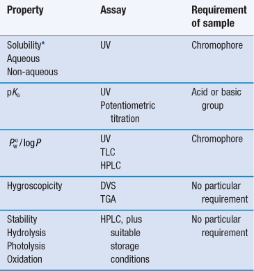
Table 23.2
Macroscopic (bulk) properties and the techniques used to determine them
| Derived property | Technique |
| Melting point | DSC or melting point apparatus |
| Enthalpy of fusion (and so ideal solubility) | DSC |
| Physical forms (polymorphs, pseudo-polymorphs or amorphous) | DSC, XRPD, microscopy |
| Particle shape Size distribution Morphology Rugosity Habit |
Microscopy Particle sizing BET (surface area) |
| Density Bulk Tapped True |
Tapping densitometer |
| Flow | Angle of repose |
| Compressibility | Carr’s index Hausner ratio |
| Excipient compatibility | HPLC, DSC |
The full characterization of a drug candidate (in the context of preformulation) should be possible with just ultraviolet (UV) spectroscopy, high-performance liquid chromatography (HPLC), differential scanning calorimetry (DSC), dynamic vapour sorption (DVS) and X-ray powder diffraction (XRPD). This explains the popularity of these techniques in pharmaceutical development. Thin-layer chromatography (TLC) and thermogravimetric analysis (TGA) provide useful supporting data, but neither is essential during the early stages.
Solubility
Aqueous solubility is a critical attribute. No drug will reach its ultimate therapeutic target without first being in solution. Consequently, it is the first physicochemical parameter to be determined. It has been estimated that, historically, up to 40% of drug candidates have been abandoned because of poor aqueous solubility, and between 35–40% of compounds currently in development have an aqueous solubility below 5 mg mL−1 at pH 7. The USP and PhEur provide definitions of solubility based on concentration (see Chapter 2 and in particular, Table 2.2).
Early determination of solubility gives a good indicator as to the ease of formulation of a drug candidate. Initial formulations, used for obtaining toxicity and bioavailability data in animal models, will need to be liquids for oral gavage or intravenous delivery, and a solubility above 1 mg mL−1 is usually acceptable. For the final product, assuming oral delivery in a solid form, solubility of the molecule above 10 mg mL−1 is preferable. If the solubility of the drug candidate is less than 1 mg mL−1 then salt formation, if possible, is indicated. Where solubility cannot be manipulated through salt formation, then a novel dosage form will be required.
Dissolution is a phase transition and in order to progress, solid-solid bonds must be broken (effectively, the solid melts), while solvent-solvent bonds must be broken and replaced by solute-solvent bonds (the drug molecules become solvated) (Chapter 2). With excess solid present, a position of equilibrium will be established between the solid and dissolved drug.
The concentration of drug dissolved at this point is known as the equilibrium solubility (usually referred to simply as solubility) and the solution is saturated. If the drug has an ionizable group then the equilibrium solubility of the unionized form is called the intrinsic solubility (So). This is important, because ionizable drugs will dissociate to a greater or lesser extent, influenced by solution pH, and this will affect the observed solubility.
From a thermodynamic perspective, the energy input required to break the solid-solid bonds must equal the enthalpy of fusion (ΔHf) required to melt the solid (since the same bonds are broken). Unlike melting, however, in the case of dissolution there is an additional enthalpy change because solvent-solvent bonds are broken and solute-solvent bonds are formed (shown diagrammatically in Fig.2.2). The energy involved in this process is known as the enthalpy of mixing (ΔHmix). The net enthalpy of dissolution (ΔHsol) is thus the sum of the enthalpy of fusion and the enthalpy of mixing:
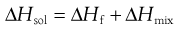 (23.1)
Knowledge of this relationship between solubility and bond energy can be used during preformulation to make predictions of solubility from thermal energy changes (e.g. during melting and other phase changes).
Thus, dissolution in the presence of a solid results in an equilibrium between the solid and the dissolved state. The equilibrium constant (Ksol) for the overall process of dissolution can be represented as:
 (23.2)
where a denotes the activity of the drug in solution aaq and in the solid phase as. Since the activity of a solid is defined as unity and in dilute solution activity approximates to concentration (solubility in this case) then:
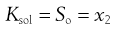 (23.3)
where So is again the intrinsic solubility and x2 denotes the saturated concentration of drug in mole fraction units (x1 being the mole fraction of the solvent).
It is possible to see from Equation 23.1 that the crystal lattice energy might affect solubility. There will also be an effect of temperature on solubility, since the position of the equilibrium between solid and dissolved drug will change. Both of these effects can be explored further through the concept of ideal solubility.
Ideal solubility
In the special case where the energy of the solute-solvent bond is equal to the energy of the solvent-solvent bond, then solute-solvent bonds may form with no change in intermolecular energy (i.e. ΔHmix = 0) and dissolution is said to be ideal. Ideal dissolution (although unlikely in reality) leads to ideal solubility and is an interesting theoretical position because it can be described in thermodynamic terms that allow calculation of the dependence of solubility with temperature.
From Equation 23.1, if ΔHmix = 0 then ΔHf is equal to ΔHsol. Incidentally, since ΔHf must be positive (i.e. endothermic) ΔHsol must also be positive for ideal dissolution. For a process to occur spontaneously the Gibbs free energy (ΔG) must be negative. The familiar thermodynamic relationship for dissolution is:
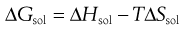 (23.4)
where T is temperature. ΔGsol is most likely to be negative when ΔHsol is negative but, as noted above, ΔHsol is frequently positive for dissolution. This means that for dissolution to occur spontaneously, the driving force must be an increase in entropy.
Equation 23.3 shows that solubility has the attributes of an equilibrium constant. This being so, it is possible to apply the van’t Hoff equation (Eqn 23.9), yielding:
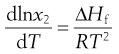 (23.5)
Making the assumption that ΔHf is independent of temperature, then integrating Equation 23.5 from Tm to T results in:
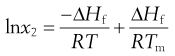 (23.6)
where Tm is the melting temperature of the pure drug and T is the experimental temperature.
Equation 23.6 is very useful in preformulation, since it allows prediction of ideal solubility at a particular temperature if the melting temperature and enthalpy of fusion of the pure drug are known. This is why determination of melting point and enthalpy of fusion are the next physicochemical parameters to be determined during preformulation.
Determination of melting point and enthalpy of fusion using differential scanning calorimetry
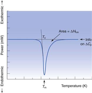
The energy changes discussed above can be measured by differential scanning calorimetry (DSC). In DSC, the power required to heat a sample in accordance with a user-defined temperature program is recorded, relative to an inert reference. The heating rate (β) can be linear or modulated by a mathematical function. When the sample melts, energy will be absorbed during the phase change and an endothermic peak will be seen, Figure 23.1. The enthalpy of fusion is equal to the area under the melting endotherm while the melting temperature may be determined either as an extrapolated onset (To) or the peak maximum (Tm).
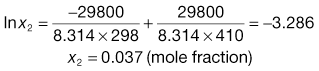
Box 23.1 Worked example
The melting temperature of aspirin is 137 °C and its enthalpy of fusion at the melting temperature is 29.80 kJ mol−1. What is the ideal solubility of aspirin at 25 °C?
Applying Equation 23.6:
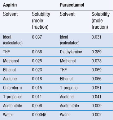
Invariably, real solutions do not show ideal behaviour because the assumptions made earlier that ΔHmix = 0 and that ΔHf is independent of temperature are not always valid. A negative (exothermic) enthalpy of mixing increases solubility, while a positive (endothermic) enthalpy of mixing reduces solubility. Table 23.3 lists the experimentally measured solubilities for aspirin and paracetamol in a range of solvents. Note that solubility in water is by far the lowest of any of the solvents shown, while solubilities in tetrahydrofuran (THF) and methanol approach ideality in the case of aspirin, and exceed ideality in the case of paracetamol.
The reason that so many solvents, and water in particular, display such non-ideal behaviour is because of significant intermolecular bonding resulting from their chemical structure and properties. The three primary chemical properties are the dipole moment, dielectric constant and capacity for forming hydrogen bonds.
A molecule has a dipole when there is a localized net positive charge in one part of the molecule and a localized net negative charge in another. Such molecules are said to be polar. Water is an example of a polar molecule. Drugs that have dipoles or dipolar character are generally more soluble in polar solvents.
Dielectric properties are related to the capacity of a molecule to store a charge and are quantified by a dielectric constant. Polar solvents may induce a dipole in a dissolved solute, which will increase solubility. The dielectric constants of a number of commonly used pharmaceutical solvents are given in Table 23.4. It can be seen that water has a high dielectric constant (78.5) relative to that of methanol (31.5) even though both are considered to be polar solvents.
Table 23.4
Dielectric constants of some common pharmaceutical solvents at 25 °C
| Solvent | Dielectric constant (no units, dimensionless) |
| Water | 78.5 |
| Glycerin | 40.1 |
| Methanol | 31.5 |
| Ethanol | 24.3 |
| Acetone | 19.1 |
| Benzyl alcohol | 13.1 |
| Phenol | 9.7 |
| Ether | 4.3 |
| Ethyl acetate | 3.0 |
Hydrogen bonding occurs when electronegative atoms (such as oxygen) come into close proximity with hydrogen atoms; electrons are pulled towards the electronegative atom creating a reasonably strong force of interaction. A drug that has a functional group capable of hydrogen bonding with water (such as —OH, —NH or —SH) should have increased aqueous solubility.
Solubility as a function of temperature
Equation 23.6 indicates that the heat of fusion should be determinable by experimentally measuring the solubility of a drug at a number oftemperatures (since a plot of lnx2 versus  should be linear and have a slope of
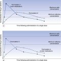
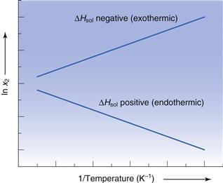
  ). Since ΔHfmust be positive, Equation 23.6 suggests that the solubility of a drug should increase with an increase in temperature. Generally, this agrees with everyday experience, but there are some drugs for which solubility decreases with increasing temperature. This is because an assumption was made in deriving Equation 23.6, namely that ΔHf was equal to ΔHsol. However, as noted above and as demonstrated by the data in Table 23.3, ΔHmix is frequently not zero. In cases where ΔHsol is negative (i.e. the heat of solution is exothermic), solubility will decrease with increasing temperature. These effects are shown in Figure 23.2.
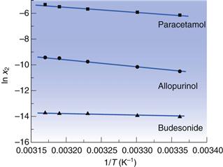
Examples of data from three drug molecules plotted this way are given in Figure 23.3. While such plots are frequently found to be linear, they are usually plotted over a very narrow temperature range and the heat of fusion so calculated is rarely ideal, although it can be considered to be an approximate heat of solution.
 for three drugs in water.
 Solubility and physical form
If molecules in the solid state are able to align in different patterns (the phenomenon of polymorphism, Chapter 8), then it is highly likely that the strength of the intermolecular bonds, and hence crystal lattice energy, will vary. Two polymorphs of the same drug will thus have different melting temperatures and heats of fusion. Usually the stable polymorph has the highest melting point and greatest heat of fusion and so, from Equation 23.6, the lowest solubility. Any metastable forms will, by definition, have lower melting points, lower enthalpies of fusion and so greater solubilities. The amorphous form, by virtue of not possessing a melting point, will have the greatest solubility. It is therefore clear that the solid-state structure of a new drug candidate should be determined during preformulation.
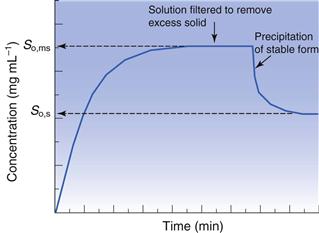
As discussed above, solubility is defined as the equilibrium between dissolved solute and the solid form. Thus, if a saturated solution is prepared by dissolving a metastable form and the excess solid is removed by filtration, the solution will be supersaturated with respect to the stable form. Ultimately, the stable form will precipitate as the system re-establishes a position of equilibrium (Fig. 23.4). Formulating any drug in a (solid) metastable form thus involves an element of risk; the risk being that the stable form will appear during storage or post-dissolution. In either case solubility will be reduced with, potentially, a consequential reduction in bioavailability.
Measurement of intrinsic solubility
Initially, during preformulation, solubility should be determined in 0.1 M HCl, 0.1 M NaOH and water. These ‘unsophisticated’ choices are determined by the scarcity of material at this stage. Saturated solutions can be prepared by adding an excess of solid to a small volume of solvent, agitating with time and then filtering.
Ultraviolet (UV) spectroscopy is the first choice assay, for reasons of familiarity, cost, the small volume of solution needed and the fact that the majority of drugs contain at least one functional group that absorbs in the UV region (190–390 nm). Table 23.5 lists the UV absorbance maxima for a series of common functional groups (called chromophores).
Table 23.5
UV absorbance maxima for a range of common functional groups
| Chromophore | λmax (nm) | Molar extinction (ε) |
| Benzene | 184 | 46700 |
| Naphthalene | 220 | 112000 |
| Anthracene | 252 | 199000 |
| Pyridine | 174 | 80000 |
| Quinoline | 227 | 37000 |
| Ethlyene | 190 | 8000 |
| Acetylide | 175–180 | 6000 |
| Ketone | 195 | 1000 |
| Nitroso | 302 | 100 |
| Amino | 195 | 2800 |
| Thiol | 195 | 1400 |
| Halide | 208 | 300 |
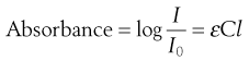
Excitation of the solute with the appropriate wavelength of light will reduce the amount of light passing through the solution. If the original light intensity is I0 and the amount of light passing through the sample (the transmitted light) is I, then the amount of light absorbed will be a function of the concentration of the solute (C) and the depth of the solution through which the light is passing (the path length, l). This relationship is usually expressed as the Beer-Lambert equation:
 (23.7)
where ε is a constant of proportionality called the ‘molar extinction coefficient’.
Higher values of ε mean greater UV absorbance by the solute. Values of ε for a range of functional groups are given in Table 23.5; it can be seen that groups containing large numbers of delocalized electrons, such as those containing benzene rings, have much greater ε values that groups containing simple carbon-carbon double bonds. The absorbance of a chromophore can be affected by the presence of an adjacent functional group if that group has unshared electrons (an auxochrome). A list of common auxochromes and their effects on the molar extinction coefficients of their parent benzene ring is given in Table 23.6.
Table 23.6
The effect of auxochromes on the UV absorbance of the parent compound C6H5-R
| Substituent | λmax (nm) | Molar extinction (ε) |
| —H | 203.5 | 7400 |
| —CH3 | 206.5 | 7000 |
| —Cl | 209.5 | 7400 |
| —OH | 210.5 | 6200 |
| —OCH3 | 217 | 6400 |
| —CN | 224 | 13000 |
| —COO− | 224 | 8700 |
| —CO2H | 230 | 11600 |
| —NH2 | 230 | 8600 |
| —NHCOCH3 | 238 | 10500 |
| —COCH3 | 245.5 | 9800 |
| —NO2 | 268.5 | 7800 |
Measurements of UV absorbance (thus solution concentration) should be recorded until the concentration remains constant and at a maximum. Care should be taken to ensure that the drug does not degrade during testing, if hydrolysis or photolysis are potential reaction pathways, and also that the temperature does not fluctuate. If the measured solubilities are the same in the three solvents then the drug does not have an ionizable group. If solubility is highest in acid then the molecule is a (weak) base and if solubility is highest in alkali the molecule is a (weak) acid.
Solubility should be measured at a (small) number of temperatures:
| 4 °C | The reduced temperature minimizes the rate of hydrolysis (if applicable). Here, the density of water is at its greatest and thus presents the greatest challenge to solubility |
| 25 °C | Standard room temperature |
| 37 °C | Body temperature and so an indication of solubility in vivo. |
Note that possession of solubility data as a function of temperature allows (approximate) determination of the heat of fusion from Equation 23.6.
If the aim of the preformulation screen is to understand solubility in vivo, then solubility in bio-relevant media should be determined. Assuming oral delivery, typical media would include simulated gastric fluid (SGF), fed simulated intestinal fluid (FeSSIF) and/or fasted simulated intestinal fluid (FaSSIF). The use of these fluids is discussed further in Chapters 21 and 35 and details of their composition is given in Tables 35.2 and 35.3. Bio-relevant media tend to have higher ionic strengths and hence the risk of salting out via the common ion effect (see below) is greater.
Effect of impurities on intrinsic solubility
One potential consideration at this stage is the polymorphic form of the drug, which may initially be present in a metastable form. It is a good idea to use differential scanning calorimetry (DSC) or X-ray powder diffraction (XRPD) to determine the polymorphic form of the excess solid, filtered from the solubility experiments, to ensure there has been no form change to a stable polymorph, or that a hydrate has not formed (since both forms typically have lower solubilities).
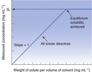
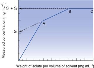
Another issue for consideration at this stage is the chemical purity of the sample. If the drug is pure, then its phase-solubility diagram should appear as in Figure 23.5. Initially, all drug added to the solvent dissolves and the gradient of the line should be unity. When saturation is achieved, addition of further drug does not result in an increase in concentration and the gradient becomes zero. However, new drug candidate material is rarely pure. When a single impurity is present, the phase-solubility diagram will appear as shown in Figure 23.6. From the origin to point A both components dissolve. At point A the first compound has reached its solubility. The line AB represents the continued dissolution of the second compound. At point B the second compound reaches its solubility and the gradient of the line BC is zero. The solubility of the first compound (S1) can be determined by extrapolation of line AB to the y-axis. The solubility of the second compound (S2) is the difference between the solubility at BC (= S1 + S2) and the y-intercept of the extrapolated line AB. The same principles apply if further impurities are present.
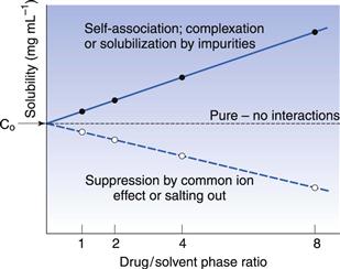
An alternative experiment is to prepare four solutions of the drug candidate with different phase-ratios of drug to solvent (say 3, 6, 12 and 24 mg of drug in 3 mL), measure the solubility of each and then extrapolate the data to a theoretical phase-ratio of zero (Fig. 23.7). If the drug is pure then solubility should be independent of phase-ratio. If the impurity acts to increase solubility (for instance, by self-association, complexation or solubilization), then the gradient of the plotted line will be positive, whereas if the impurity acts to suppress solubility (usually by the common ion effect) then the gradient of the line will be negative. The point at zero phase ratio in Figure 23.7 implies that the impurity concentration is zero and thus the true solubility can be estimated.
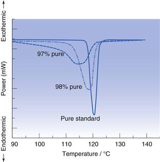
The purity of a sample may also be checked with DSC, since the presence of an impurity (even minor amounts) will lower and broaden the melting point of a material. Qualitatively, if the melting endotherm recorded using DSC is very broad, then the sample is likely to be impure (see Fig. 23.8).
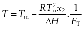
If the melting point and heat of fusion of the pure drug are known, then the purity of an impure sample can be quantified by analysis of DSC data. Analysis requires determination of the fraction of sample melted as a function of temperature. This is easily achieved by recognizing that integration of the peak area of melting gives the total heat of melting (Q). Partial integration of the melting endotherm to any particular temperature must therefore give a smaller heat (q). The fraction of material melted at any temperature (FT) is then:
 (23.8)
Changes in FT values as a function of temperature are easily measured. The van’t Hoff equation (Eqn 23.9) predicts that a plot of  versus temperature should be a straight line of slope
  , from which the mole fraction of the impurity (x2) can be calculated.
 (23.9)
Molecular dissociation
Approximately two-thirds of marketed drugs ionize between pH 2 and 12 (analysis of the 1999 World Drug Index by Manallack, 2007). Understanding acid and base behaviour is thus extremely important, not only because of the number of ionizable drugs available, but also because the solubility of an acidic or basic drug will be pH-dependent (and because possession of an ionizable group opens the possibility of solubility manipulation via salt formation). Determining the pKa of a drug is the next step in preformulation characterization. This is particularly important with drugs intended for peroral administration as they will experience a range of pH environments, and it is important to know how their degree of ionization may change during passage along the gastrointestinal tract.
The principles of acid-base equilibria are discussed in Chapter 3, where the Henderson-Hasselbalch equations (Eqns 3.15 and 3.19) were derived for acid and base species.
The Henderson-Hasselbalch equations allow calculation of the extent of ionization of a drug as a function of pH, if the pKa is known. When the pH is significantly below the pKa (by at least 2 pH units), a weakly acidic drug will be completely unionized and when the pH is significantly above the pKa (by at least 2 pH units) a weakly acidic drug will be fully ionized (and vice versa for a basic drug) (see Fig. 3.1).
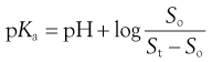
The degree of ionization will affect solubility because ionized species are more freely soluble in water. Taking the acid-species Henderson-Hasselbalch equation as an example (i.e. Eqn 3.15), since [A−] represents the saturated concentration of ionized drug (Si) and [HA] represents the saturated concentration of unionized drug (i.e. the intrinsic solubility, So) then the equation may be re-written as:
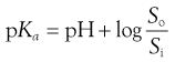 (23.10)
At any given pH, the observed total solubility (St) must be the sum of the solubilities of unionized and ionized fractions, i.e.:
 (23.11)
Note that in this chapter, the alternative symbol S (with appropriate subscript) is used for the specific concentration of solution that corresponding to the saturated concentration or ‘solubility. This is equally acceptable and is presented here, and later in the discussion of intrinsic dissolution rate, as an alternative to annotation used elsewhere. This annotation is particularly useful when discussing various types of solubility, as here.
Rearranging Equation 23.11 gives:
 (23.12)
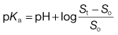
Substituting in Equation 23.10 gives:
 (23.13)
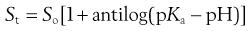
Or, in antilog form:
 (23.14)
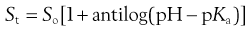
Equation 23.14 allows calculation of the total solubility of an acidic drug as a function of pH. Total solubility will be equal to the intrinsic solubility at pH values below pKa and will increase significantly at pH values above pKa. In theory, Equation 23.14 predicts an infinite increase in solubility when pH >> pKa. In practice this is not attained, primarily because real systems exhibit non-ideal behaviour. Nevertheless, Equation 23.14 is a useful approximation over narrow, but useful, pH ranges.
A similar derivation can be made for weak bases following the same logic, resulting in:
 (23.15)
Equation 23.15 implies that, for weak bases, total solubility will be equal to the intrinsic solubility at pH values above pKa and will increase significantly at pH values below pKa.
Measurement of pKa
Modern automated instrumentation is available that can determine pKa values with very small (typically 10–20 mg) amounts of drug. This is extremely useful in the context of preformulation where material is scarce. Usually this instrumentation is based upon a potentiometric pH titration. The drug is dissolved in water, forming either a weakly acidic or weakly basic solution. Acid or base (as appropriate) is titrated and the solution pH recorded. A plot of volume of titrant solution added versus pH allows graphical determination of the pKa, since when pH = pKa the compound is 50% ionized. This method has the significant advantage of not requiring an assay.
Alternative methods for determining pKa include conductivity, potentiometry and spectroscopy. However, if the intrinsic solubility has been determined, measurement of solubility at a pH where the compound is partially ionized will allow calculation of pKa from the Henderson-Hasselbalch equations.
Box 23.2 Worked example
What is the pKa of chlordiazepoxide given the following solubility data? So = 2 mg mL−1, St at pH 4 = 14.6 mg mL−1 and St at pH 6 = 2.13 mg mL−1.
For a weak acid,
At pH 4:
At pH 6:
The literature value is 4.8.
Partitioning
No solute has complete affinity for either a hydrophilic or a lipophilic phase. In the context of preformulation, it is important to know early in the development stage how a molecule (or charged ion) will distribute between aqueous and fatty environments (e.g. between gut contents and lipid biological bilayers in the surrounding cell walls). When a solute is added to a mixture of two (immiscible) solvents it will usually dissolve in both to some extent and a position of equilibrium will be established between the concentrations (C) in the two solvents. In other words, the ratio of the concentrations will be constant and is given by:
 (23.16)
where P is the partition coefficient and the superscript and subscript indicate the solvent phase. Note that it would be equally possible to define:
 (23.17)
In a physiological environment, drugs partition from an aqueous phase to numerous and complex lipophilic phases (typically various cell membranes, see also Chapter 21). It would be difficult to develop an analytical method that allowed measurement of actual partitioning between such complex phases and so a simple solvent model, commonly using n-octanol, is usually used instead. n-Octanol is taken to mimic the short-chain hydrocarbons that make up many biological lipid bilayers. A partition coefficient for the partitioning of a solute between water (w) and n-octanol (o) can be written as:
 (23.18)
Alternatively, the following could be defined:
 (23.19)
By convention  is the standard term.
When a drug is lipophilic (i.e. it has a high affinity for the octanol phase) the value of  will be greater than 1 and when the drug is hydrophilic the value of
  will be less than 1. Since hydrophilic drugs will give very small
  values,
  values are often quoted (abbreviated to log P), in which case hydrophilic drugs will have a negative value and lipophilic drugs a positive value.
Note that since only unionized solute can partition (ionized species are too polar to dissolve in organic phases), the partition coefficient applies only if (a) the drug cannot ionize or (b) the pH of the aqueous phase is such that the drug is completely unionized. If the drug has partially ionized in the aqueous phase and partitioning is measured experimentally, then the parameter measured is the distribution coefficient, D:
 (23.20)
The partition coefficient and the distribution coefficient are related by the fraction of solute unionized (funionized):
 (23.21)
Note also that partition coefficients may be defined between any organic phase and water. n-Octanol is the most common choice, but it is by no means either the best choice, nor the only choice for the ‘oil’ phase, especially if partition coefficients are determined using chromatographic methods. However, much data exists for n-octanol/water systems and its use continues.
Determination of log P
Log P values can be determined experimentally or can be calculated from the chemical structure of the drug candidate using group additivity functions. For the latter approach there are numerous computer models and simulation methods available; selection will reduce to personal choice and familiarity and so these models will not be considered here. Rather, this text will focus on experimental determination. It is clear, however, that there is much value to be gained by comparing calculated and experimentally determined log P values. The value of the calculation approach is greatest when selecting a lead candidate from a compound library when it would simply be neither possible, nor practicable to measure the partitioning behaviour of the many thousands of compounds available.
Shake-flask method
Assuming that a UV assay is available, the shake-flask method is a quick, simple and near universally applicable way of determining the partition coefficient (see also Fig. 21.2). Prior to measurement, the solvents to be used should be mixed with each other and allowed to reach equilibrium. This is because each solvent has a small but significant solubility in the other (n-octanol in water is 4.5 × 10⁻³ M; water in n-octanol is 2.6 M).
The drug is dissolved in the aqueous phase to a known concentration. Equal volumes of aqueous drug solution and n-octanol are then mixed in a separating funnel. The mixture is shaken vigorously for a period of time (usually 30 minutes, to maximize the surface area of the two solvents in contact with each other) while the drug partitions. The phases are allowed to separate (5 minutes) and then the concentration of drug remaining in the aqueous phase is determined, Figure 23.9. By difference, the concentration of drug in the n-octanol phase is known:
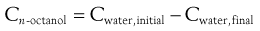 (23.22)
When the partition coefficient heavily favours distribution to the n-octanol phase, then a smaller volume of n-octanol can be used, since this will increase the concentration in the aqueous phase at equilibrium, reducing the error in the analytical determination of the concentration. The calculation for partition coefficient needs to be corrected to account for the different volumes. For example, assuming a 1 : 9 n-octanol:water ratio, Equation 23.18 becomes:
 (23.23)
There are some drawbacks to the shake-flask method. One is that the volumes of solution are reasonably large and another is that sufficient time must be allowed to ensure equilibrium partitioning is attained.
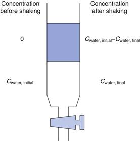
The use of n-octanol tends to reflect absorption from the gastrointestinal tract, which is why it is the default option; but n-octanol may not be the best organic phase. Hexane or heptane can be used as alternatives, although they will give different partition coefficient values from n-octanol and are also considered to be less representative of biological membranes because they cannot form any hydrogen bonds with the solute. Where the aim of the experiment is to differentiate partitioning between members of a homologous series the organic phase can be varied in order to maximize discrimination. n-Butanol tends to result in similar partition values for a homologous series of solutes, while heptane tends to exaggerate differences in solute lipophilicity. Solvents that are more polar than n-octanol are termed hypo-discriminating and those that are less polar than n-octanol are termed hyper-discriminating. Hyper-discriminating solvents reflect more closely transport across the blood-brain barrier, while hypo-discriminating solvents give values consistent with buccal absorption. The discriminating powers of a range of common solvents, relative to n-octanol, are shown in Figure 23.10.
Chromatographic methods
Separation of analytes by liquid chromatographic methods relies on interaction between the analytes (dissolved in a mobile phase) and a stationary (solid) phase. In normal-phase chromatography, the stationary phase is polar and the mobile phase is non-polar, and in reverse-phase chromatography the stationary phase is non-polar and the mobile phase is polar. It follows that liquid chromatography may be used with single analytes to measure partitioning behaviour, since the extent of interaction must depend upon the relative lipophilicity or hydrophilicity of the analyte. Typically, reverse-phase chromatography is used for partitioning experiments.
Reverse-phase thin-layer chromatography (TLC) allows measurement of partition coefficients by comparing progression of a solute relative to progression of the solvent front (the ratio of the two being the resolution factor, Rf). The resolution factor achieved for each drug is converted to a TLC retention factor (Rm), which is proportional to log P.
 (23.24)
The stationary phase can be n-octanol but is more commonly silica impregnated with silicone oil. The mobile phase can in principle be water (or aqueous buffer), but unless the solute is reasonably hydrophilic, good resolution tends not to be achieved with water alone and reasonably lipophilic compounds tend not to move from the ‘starting line’ at all (i.e. Rf = 0). Co-solvents (typically acetone, acetonitrile or methanol) can be added to the mobile phase to increase the migration of highly lipophilic compounds. The nearer the compound migrates to the solvent front, the higher the resolution factor (the maximum value attainable being 1). The value of Rf can in principle vary between 0 and 1 (corresponding to Rm values from +∞ to −∞, respectively) although in practice the measurable range is about 0.03 to 0.97, corresponding to Rm values of 1.5 to −1.5, respectively.
Addition of a co-solvent can be used to modulate the value of Rf obtained and the relationship is usually linear. This being so, it is possible to extrapolate to zero co-solvent and so calculate Rm in water.
Reverse-phase HPLC is an alternative, and widely used, technique for measurement of partition coefficients. The stationary phase comprises a non-polar compound (typically a C18 hydrocarbon) chemically bound to an inert, solid support medium (such as silica). It is possible to use water saturated with n-octanol as the mobile phase, and a stationary phase covered in n-octanol, but the eluting power is not strong, for the same reason noted above for TLC, and so to measure an acceptable range of partition coefficients it is necessary to change the volume ratio of mobile to stationary phase.
Because the hydrocarbon is bound to a solid substrate it cannot behave as a true liquid phase and so conceptually it is not clear whether the interaction between the solute and the stationary phase constitutes surface adsorption or true phase partitioning. While C18 hydrocarbons have been found to provide a better correlation to log P values, indicating that their greater reach from the solid surface of the support matrix means they behave more like a liquid phase, true partitioning is unlikely to occur.
Dissolution rate
Knowledge of solubility per se does not inform dissolution rate, since solubility is a position of equilibrium and not the speed at which it is attained. Thus, high aqueous solubility does not necessarily mean that a compound will exhibit satisfactory absorption. Absorption can be assumed to be unimpeded if a drug candidate has an intrinsic dissolution rate (IDR – see below) greater than 1 mg cm−2 min−1.
Intrinsic dissolution rate
One assumption in the use of the Noyes and Whitney equation (described in Chapter 2, Eqns 2.3 and 2.4) is that the parameters of diffusion coefficient (D), the surface area of dissolving solid (A) and the thickness of the stationary solvent layer surrounding the dissolving solid (h) remain constant. Assuming a constant stirring speed and that the solution does not increase in viscosity as the solid dissolves, this is appropriate for D and h but A must always change as the solid dissolves (see Fig. 2.4). Also, if a tablet disintegrates, for instance, then A would increase rapidly at the start of dissolution before decreasing to zero, and there will be a concomitant effect on the dissolution rate.
If the sample is constructed such that A remains constant throughout dissolution, and sink conditions are maintained so that (St − C) ≅ St (see above), then the measured rate is called the intrinsic dissolution rate (IDR) (see also Chapter 2 and Eqn 2.6):
 (23.25)
Wells (1988) suggests a method for measuring the IDR of a compound. A compact of the drug (300 mg) is prepared by compression (to 10 tonnes load) in an infrared punch and die set (13 mm diameter, corresponding to a surface area on the flat face of 1.33 cm2). The metal surfaces of the punch and die should be pre-lubricated with a solution of stearic acid in chloroform (5% w/v). The compact is adhered to the holder of the rotating basket apparatus using low-melting paraffin wax. The compact is repeatedly dipped into the wax so that all sides are coated except the lower flat face (from which any residual wax should be removed with a scalpel blade). Dissolution is recorded while the disc is rotated (100 rpm) 20 mm from the bottom of a flat-bottomed dissolution vessel containing dissolution medium (1 L at 37 °C). The gradient of the dissolution line divided by the surface area of the compact gives the IDR.
IDR as a function of pH
Measurement of IDR as a function of either pH or ionic strength can give a good insight into the mechanism of drug release and the improvement in performance of salt forms, since, for weak acids, substitution of Equation 23.14 into Equation 23.25 yields:
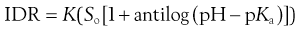 (23.26)
And for weak bases substitution of Equation 23.15 into Equation 23.25 yields:
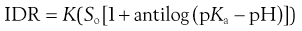 (23.27)
In either case, the measured IDR will clearly be affected either by the pH of the medium or the microenvironment surrounding the solid surface created by the dissolving salt. The effect of pH on IDR is easily established by selection of the dissolution media. Standard media (0.1M HCl, phosphate buffers, etc.) can be used or, in order to get a more realistic insight into dissolution in vivo, simulated gastrointestinal fluids (as discussed earlier) can also be employed.
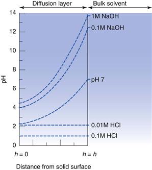
If the drug is an acid or base, then the self-buffering effect as dissolution occurs should not be ignored. In particular, the saturated concentration of solute in the diffusion layer often means that the pH in the medium immediately surrounding the dissolving solid differs significantly from that of the bulk solvent and will lead to deviations from the ideal behaviour predicted by Equations 23.26 and 23.27. A schematic representation of the buffering effect of salicylic acid is shown diagrammatically in Figure 23.11.
IDR and the common ion effect
The common ion effect (discussed in Chapter 2) should not be ignored, especially for hydrochloride salts, as the chloride ion is often present in reasonably high concentrations in body fluids (0.1 M in gastric fluid and 0.13 M in intestinal fluid). For this reason, fed and fasted simulated intestinal fluids should contain 0.1 and 0.2 M Cl− respectively.
Hence, when the concentration of Cl− in solution is high, the solubility advantage of choosing a hydrochloride salt is diminished. Li et al (2005) demonstrated the effect of chloride concentration on the IDR of haloperidol salts and showed that dissolution of the hydrochloride salt was slower than that of a either the phosphate or mesylate salt.
Salt selection
If a drug candidate has poor aqueous solubility or is difficult to isolate or purify, but is a weak acid or base, then conversion to a salt form may be beneficial. A number of physicochemical properties may change upon formation of a salt (Table 23.7). Any such changes may be beneficial or detrimental and so a decision must be made early during preformulation as to which salt form (if any) is to be taken into development. This decision will not depend on solubility alone. The prevalence of salt forms of drugs in practice (estimated at around 50%) suggests that the benefits often outweigh the drawbacks. Salt selection should preferably be made before commencement of toxicity testing, because of the associated cost and potential time delay in development of switching to a different salt form. Each is treated by regulatory authorities as a new entity.
Table 23.7
| Advantages | Disadvantages |
| Enhanced solubility | Decreased percentage of active |
| Increased dissolution rate | Increased hygroscopicity |
| Higher melting point | Decreased chemical stability |
| Lower hygroscopicity | Increased number of polymorphs |
| Improved photostability | Reduced dissolution in gastric media |
| Better taste | No change in solubility in buffers |
| Higher bioavailability | Corrosiveness |
| Better processability | Possible disproportionation |
| Easier synthesis or purification | Additional manufacturing step |
| Potential for controlled release | Increased toxicity |
Salt formation
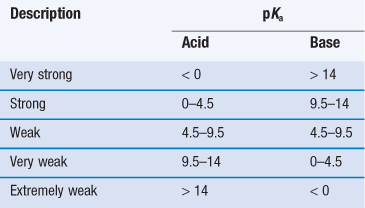
A salt is formed when an acid reacts with a base, resulting in an ionic species held together by ionic bonds. In principle, any weak acid or base can form a salt, although in practice if the pKa of the base is very low, the salt formed is unlikely to be stable at physiological pHs. Stephenson et al (2011) note that no marketed salt exists for a drug with a pKa below 4.6. They suggested that 5 is a general value below which salt formation is unlikely to be effective. Because salts usually dissociate rapidly upon dissolution into water, they are considered electrolytes. Sometimes a drug sounds from its name that it is a salt, but it may in fact be a single entity bound via covalent bonds, in which case electrolytic behaviour does not apply (e.g. fluticasone propionate).
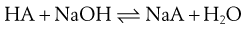
Acids and bases can be classified as strong through to extremely weak, based on their pKa (Table 23.8). When strong acids react with strong bases the reaction tends to completion, as both species will be fully ionized, and this is known as neutralization. For example:
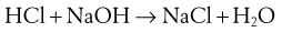 (23.28)
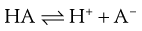
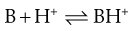
In this instance, the salt formed will precipitate once it is present at a concentration beyond its solubility. However, most drug candidates are either weak acids or bases, in which case their character is usually based on the Brønsted-Lowry definition: an acidic compound is a proton donor and a basic compound is a proton acceptor. The removal of a proton from an acid produces a conjugate base (A−) and addition of a proton to an acceptor produces a conjugate acid (BH+).
 (23.29)
 (23.30)
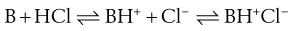
Note that the Brønsted-Lowry definition requires acidic species to have an ionizable proton but does not require basic compounds to possess a hydroxide group; simply that they can accept a proton (thus the theory does not consider KOH and the like to be a base but a salt containing the basic OH− moiety). In the case of a weak base (B) reacting with a strong acid, the conjugate acid and conjugate base may then form a salt:
 (23.31)
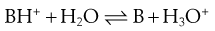
When a salt dissolves in water it will dissociate. Assuming dissolution of a basic salt then the species in solution is the conjugate acid. The conjugate acid can donate its proton to water, reforming the free base:
 (23.32)
All of the reasons for the change in solubility of salts are encompassed in Equation 23.32. A basic salt contains the conjugate acid of the drug. Upon dissolution, the conjugate acid donates its proton to water and the free base is formed. The solute is thus the free base, but the pH of the solution in which it is dissolved has reduced because of the donated proton. Recall that the solubility of weak bases increases as the pH of solution reduces. Thus, dissolution of a basic salt increases solubility because there is a concomitant reduction in pH of the solution.
The pH of a solution of a dissolved acid is given by:
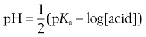 (23.33)
and, because the acid species is BH+, then:
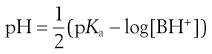 (23.34)
Box 23.3 Worked example
What is the pH of a 0.2 M solution of ergotamine tartrate (pKa 6.25)?
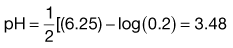
From Equation 23.34
A similar situation occurs for the reaction of a weak acid with a strong base:
 (23.35)
Upon dissolution of an acidic salt the conjugate base is formed:
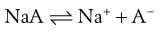 (23.36)
The conjugate base can then accept a proton from water, re-forming the free acid and increasing the pH of the solution:
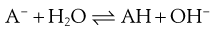 (23.37)
The solute is thus the free acid, but the pH of the solution in which it is dissolved has increased because of the generated hydroxide ion. Recall again that the solubility of weak acids increases as the pH of solution increases.
The pH of a solution of base is given by:
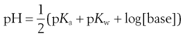 (23.38)
and since A− is a conjugate base then:
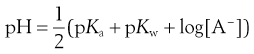 (23.39)
where pKw reflects the ionization potential of water (and is equal to 14 at 25 °C).
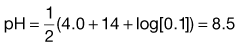
Box 23.4 Worked example
What is the pH of a 0.1 M solution of diclofenac sodium (pKa 4.0)?
From Equation 23.39:
Several consequences arise from this discussion. One is that salt formation might not best be achieved in aqueous solution, since dissolution of a salt in water generally results in formation of the free acid or base. For this reason, salts are often formed in organic solvents. Secondly, the increase in solubility of a salt over the corresponding free acid or base is a result only of the change in pH upon dissolution. The intrinsic solubility of the free acid or base does not change. Thus, if salts are dissolved in buffered solvents there will be no difference in the solubility profile of the salt relative to the corresponding free acid or base, because the buffer will act to neutralize any change in pH.
Selection of a salt-forming acid or base
For salt formation to occur there must be a sufficient difference in pKa between the acid and base (the reactivity potential). For the transfer of a proton from an acid to a weak base, the pKa of the acid must be less than that of the weak base and vice versa. As a general rule, a difference in pKa (ΔpKa) of 3 is indicated (although salt formation can sometimes occur with smaller differences; for instance, Wells (1988) notes that doxylamine succinate forms even though ΔpKa is 0.2). The reason for this pKa difference is to ensure both species are ionized in solution, thus increasing the chance of interaction. If ΔpKa lies between 3 and zero then knowledge of ΔpKa per se is not predictive of whether salt formation will occur and if ΔpKa is less than zero then co-crystal formation is the more likely outcome.
Thus, selection of a salt-forming entity starts with knowledge of the pKa of the entity and the pKa of the drug. The pKa values of some of the most common salt forming acids and bases in water are given in Tables 23.9 and 23.10.
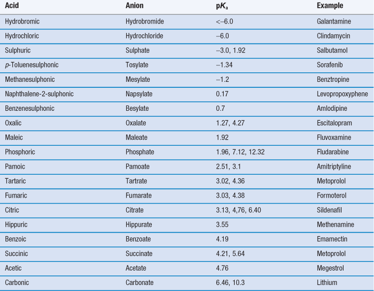
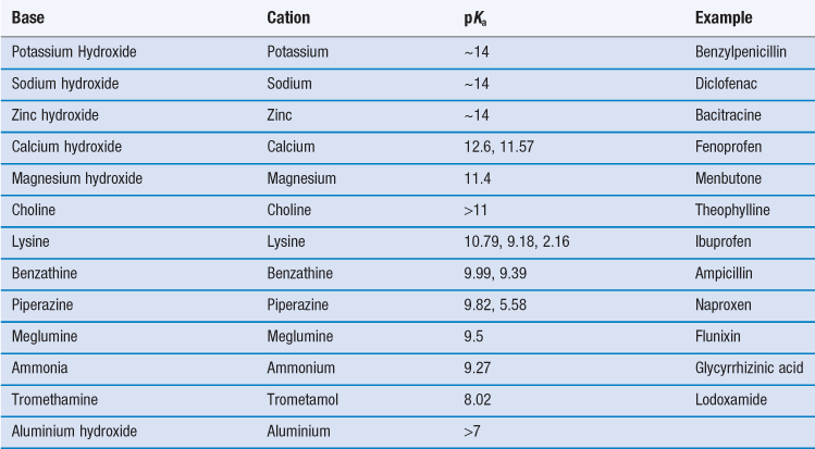
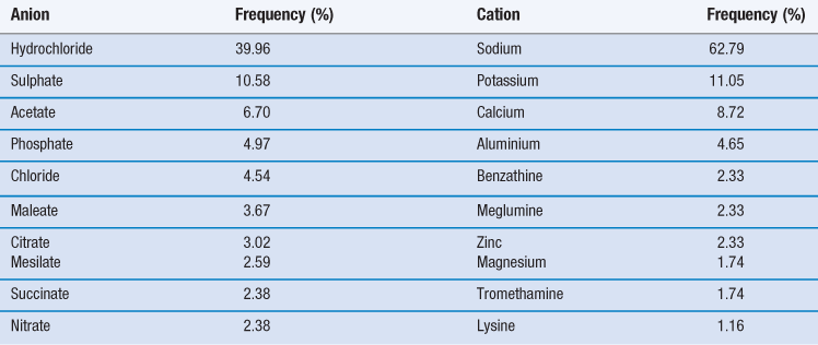
The top ten anions and cations by frequency for drugs in the 2006 USP are shown in Table 23.11. For basic drugs, the hydrochloride salt is the most common form. In part this is because the pKa of hydrochloric acid is so low it is very likely that it will form a salt with a weak base. Hydrochloride salts are also widely understood and form physiologically common ions and so are acceptable from a regulatory perspective. However, they do have some disadvantages, including the fact that the drop in pH upon dissolution may be significant (which is not good for parenteral formulations). There are also risks of corrosion of manufacturing plant and equipment, instability during storage (especially if the salt is hygroscopic) and reduced dissolution and solubility in physiological fluids because of the common ion effect.
Stahl (2011) organizes salt-formers into three categories, which may be used as a guide to selection.
First class salt-formers are those that form physiologically ubiquitous ions or which occur as metabolites in biochemical pathways. These include hydrochloride and sodium salts and, as such, they are considered to be unrestricted in their use.
Second class salt formers are those that are not naturally occurring but which have found common application and have not shown significant toxicological or tolerability issues (such as the sulphonic acids, e.g. mesilates).
Third class salt formers are those that are used in special circumstances to solve a particular problem. They are not naturally occurring, nor are they in common use.
An additional factor to consider is that the salt formed should exist as a crystalline solid, to enable ease of isolation and purification. Amorphous salts are highly likely to cause problems in development and use and so should be avoided.
Salt screening
Once potential salt formers are selected they must be combined with the free drug in order to see which preferentially form salts. Since the potential number of permutations and combinations of salt formers and solvents is large, a convenient method for salt screening at the preformulation stage is to use a micro-plate well approach. A small amount of drug (~0.5 mg) in solvent is dispensed into each well of a 96-well plate. To each well is added a solution of potential counter-ion. It is possible to construct the experiment in the well plates so that the effect of solvent is examined in the x direction and the effect of counter-ion is examined in the y direction. Solvents should be selected carefully. Commonly used solvents are listed in Table 23.12.
Table 23.12
| Solvent | Boiling point (°C) | Dielectric constant (ε) |
| N,N dimethylformamide | 153 | 37 |
| Acetic acid | 118 | 6.2 |
| Water | 100 | 78.4 |
| 1-Propanol | 97 | 20.3 |
| 2-Propanol | 83 | 19.9 |
| Acetonitrile | 82 | 37.5 |
| 2-Butanone | 80 | 18.5 |
| Ethanol | 78 | 24.6 |
| Ethyl acetate | 77 | 6.0 |
| n-Hexane | 69 | 1.9 |
| Isopropyl ether | 68 | 3.9 |
| Methanol | 65 | 32.2 |
| Acetone | 57 | 20.7 |
| Methylene chloride | 40 | 8.9 |
| Diethyl ether | 35 | 4.3 |
After an appropriate length of time, the presence in each well of salt crystals is checked with an optical device (for instance a microscope or a nephelometer). If no crystals are seen, then the plate can be stored at a lower temperature. If the reduction in temperature does not cause precipitation, then as a last attempt the temperature can be increased to evaporate the solvent (although care must be taken in this case during subsequent analysis because the isolate may contain a simple mixture of drug and salt former, rather than the salt itself).
Once a potential salt has been identified preparation can be undertaken with slightly larger sample masses (10–50 mg). XRPD may be used to get a preliminary idea of polymorphic form, while melting points may be determined with a melting point apparatus, hot-stage microscopy (HSM) or DSC. Examination with HSM, if operated under cross-polarized filters, allows visual confirmation of melting and any other changes in physical form during heating, while analysis with DSC provides the heat of fusion in addition to the melting temperature (and so allows calculation of ideal solubility). Additional analyses with TGA and DVS will provide information on water content and hygroscopicity (see below). All of these experiments can be performed if around 50 mg of salt is available.
Solubility of salts
It is not a simple matter to predict the solubility of a salt. In particular the common ion effect cannot be ignored, especially when dissolution and solubility in biological media are considered. There are many empirical approaches in the literature for estimating solubility of salts, but most require knowledge of the melting point of the salt, a value most reliably determined by preparing the salt and melting it (in which case, the salt is available for solubility determination by experiment). This section will thus consider the underlying principle of solubility pH-dependence, based on ionic equilibria and assumes that solubility would be determined experimentally using the actual salt.
Solubility of basic salts
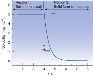
Dealing with a basic salt first, at high pH the solubility will be equal to that of the unionized (or free) base (i.e. at its lowest) and at low pH the solubility will be that of the ionized base (i.e. at its highest). There will be a region between these extremes where the solubility will vary with pH, as shown in Figure 3.1. The standard interpretation of a solubility profile of this form is based on the model of Kramer and Flynn (1972), who assumed that the overall profile is the sum of two solubility profiles (Fig. 23.12). In region 1, the dissolved solute is in equilibrium with solid salt, and in region 2 the dissolved solute is in equilibrium with solid free base. The point at which the two solubility profiles intersect is termed pHmax.
Data suggest that a basic salt will be most soluble in low pH media (such as gastric fluid) but will become increasingly insoluble as pH increases (as it would in intestinal fluids).
Solubility of acidic salts
A similar series of considerations can be made for salts of weak acids. In this case, the free acid is the solid phase in equilibrium with the saturated solution below pHmax and the salt is the solid phase in equilibrium with the saturated solution above pHmax.
An acidic salt will be least soluble in low pH media but will become increasingly soluble as pH increases. Thus, if an acidic salt is administered orally its solubility will naturally increase as it progresses along the gastrointestinal tract. Indeed a drug candidate’s solubility in gastric fluid may be so low that it will naturally dissolve only lower in the gastrointestinal tract, which may be a formulation advantage.
The importance of pHmax
At pHmax, which in principle is a single point on the solubility profile, both the free acid/base and the salt co-exist in the solid phase. For a basic salt (see Fig. 23.12), if the pH of a saturated solution containing excess solid free base is lowered below pHmax then the solid will convert to the salt (although the pH will not drop below pHmax until enough acid has been added to convert all the free base to salt). Conversely, if the pH of a saturated solution containing excess solid salt is raised above pHmax then the solid phase will convert to the free base. The opposite holds true for an acidic salt.
It should be apparent that pHmax is an important parameter and its value will change depending upon the solubility of the salt form made. In particular:
• increasing pKa by 1 unit (making the base stronger) will increase pHmax by 1 unit
• increasing the solubility of the free-base by an order of magnitude will increase pHmax by 1 unit
• increasing the solubility of the salt by an order of magnitude will decrease pHmax by 1 unit.
If a small amount of [H+] is added to the system at pHmax then free-base is converted to salt. Conversely, if alkali is added salt is converted to free-base. As the system is effectively acting as a buffer, the pH (and consequently the solubility) will not change until sufficient acid or alkali has been added to convert one solid phase completely to the other.
A similar analysis can be performed for an acidic salt. The value of pHmax can have a critical influence on the dissolution rate of salts, because the pH of the dissolution medium can cause conversion of a salt back to the free acid or base form.
Dissolution of salts
Salts have the potential to increase dissolution rate because the saturated concentration in the boundary layer is much higher than that of the free acid or base
For acidic and basic drugs, solubility is pH-dependent. Accordingly, the Noyes-Whitney model predicts that dissolution rate must therefore also be pH-dependent, with the solubility of the solute at the pH and ionic strength of the dissolution medium being the rate-controlling parameter. From the same argument, when the pH of the dissolution medium is around that of pHmax the dissolution rates of the free acid or base and its salt should be the same (because their solubilities are roughly equal at this point). There are, however, numerous examples where this is not the case, for instance doxycycline hydrochloride and doxycycline; sodium salicylate and salicylic acid; and haloperidol mesylate and haloperidol.
These differences suggest that the pH of the solution into which the solid is dissolving (i.e. the boundary layer) is materially different from that of the bulk solvent (and so the solubility of the dissolving species is different from that expected in the bulk solvent). The difference in pH between the boundary layer and bulk solvent arises because the boundary layer is a saturated solution and because dissolution of acids, bases or salts will result in a change in pH; when saturated, the pH change is maximised. Nelson (1957) first noted this correlation during a study of the dissolution of various theophylline salts; salts with higher diffusion layer pH had greater in vitro dissolution rates and, importantly, faster in vivo absorption.
The pH of the boundary layer at the surface is termed the pH microenvironment (pHmenv) and is equal to the pH of a saturated solution of the dissolving solid in water. The Noyes-Whitney equation still governs the dissolution rate, but the solubility value is not that of the solute in the dissolution medium but that in a medium of pHmenv. As the distance from the surface of the dissolving solid increases, the pH approaches that of the bulk medium (shown earlier in Fig. 23.11).
Effect of salts on partitioning
Ionized species do not partition into organic solvents or non-polar environments. Thus, while solubility may be enhanced by formation of a salt, there is a considerable risk that partitioning will decrease (example data for partitioning of the sodium salt of ibuprofen are given in Table 23.13). There is thus a compromise to be reached between increasing solubility while maintaining bioavailability and it may well be the case that on this basis, the most soluble salt is not taken forward for development.
Hygroscopicity
Hygroscopicity refers to the tendency of a substance to attract water from its immediate environment, either by absorption or adsorption. An increase in water content usually results in a change in physicochemical properties. Typically, wet powders will become more cohesive and flowability is reduced. Water also acts to mediate many solid-state reactions, so an increase in water content can often increase the rate of chemical degradation of the active or interaction with any excipients. If the substance is amorphous, then absorption of water causes plasticization of the matrix (effectively the molecular mobility of the molecules is increased) and then major structural change. If the amorphous matrix is a freeze-dried powder, then absorption of water often causes structural collapse. At the extreme, absorption of water will cause amorphous materials to crystallize.
Salts, in particular, usually have a greater propensity to absorb water than the corresponding free acid or base, so the stability of salt forms with respect to environmental humidity must be assured. Some salts (for instance potassium hydroxide or magnesium chloride) are so hygroscopic they will dissolve in the water they absorb, forming solutions. This process is called deliquescence. In any event, if water absorption is likely to cause a detrimental change in physicochemical properties, then appropriate steps must be taken to protect the drug candidate or drug product. Typically, this would involve selection of suitable packaging and advising correct storage by the patient.
From an analytical perspective, water uptake is usually determined through a change in mass (although chemical approaches, such as the Karl-Fischer titration, can also be used). Thermogravimetric analysis (TGA) measures mass as a function of temperature, whilst dynamic vapour sorption (DVS) measures mass as a function of humidity at a constant temperature. TGA thus allows determination of water content after exposure of a sample to humidity, while DVS records the change in weight of a sample during exposure to humidity.
Physical form
The solid-state is probably the most important state when considering development of a drug candidate into a drug product (discussed further in Chapter 8). Many solid-state (or physical) forms may be available and each will have different physicochemical properties (including solubility, dissolution rate, surface energy, crystal habit, strength, flowability and compressibility). In addition, physical forms are patentable, so knowing all of the available forms of a drug candidate is essential both in terms of optimizing final product performance but also in ensuring market exclusivity.
Polymorphism
When a compound can crystallize to more than one unit cell (i.e. the molecules in the unit cells are arranged in different patterns) it is said to be polymorphic (Chapter 8). The form with the highest melting temperature (and by definition the lowest volume) is called the stable polymorphic form and all other forms are metastable. Different polymorphs have different physicochemical properties, so it is important to select the best form for development. A defining characteristic of the stable form is that it is the only form that can be considered to be at a thermodynamic position of equilibrium (which means that over time all metastable forms will eventually convert to the stable form). It is tempting therefore to consider formulating only the stable polymorph of a drug, since this ensures there can be no change in polymorph upon storage. The stable form might, however, have the worst processability (for instance, the stable form I of paracetamol has poor compressibility, while the metastable form II has good compressibility), or lowest bioavailability (for instance, the presence of the B or C forms of chloramphenicol palmitate dramatically reduces bioavailability). Selection of polymorphic form is not necessarily straightforward although if the stable polymorph shows acceptable bioavailability then it is of course the best option for development.
Polymorphism screening
Polymorph screening at the preformulation stage is performed in much the same manner as described earlier for salt screening. Basic screening is achieved by crystallizing the drug candidate from a number of solvent or solvent mixtures of varying polarity. A small amount of drug (around 0.5 mg) is added into each well of a 96-well plate. To each well is added a small volume of each solvent or solvent mixture. After an appropriate length of time, the presence in each well of crystals is checked with an optical device (for instance a microscope or a nephelometer), using the strategies described previously for salt screening to facilitate crystallization.
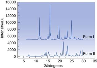
X-ray powder diffraction (XRPD) provides structural data to identify and differentiate polymorphs. Figure 23.13 shows the powder diffractograms for two polymorphs of sulfapyridine; it is immediately apparent that each has a unique set of intensity peaks and so the forms are qualitatively different. The 2θ angles for each peak provide a ‘fingerprint’ for each form, while the intensities of each peak can be used as the basis for a quantitative assay for each form.
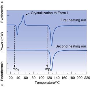
Differential scanning calorimetry (DSC) data differentiate polymorphs on the basis of their melting points and heats of fusion, thus providing thermodynamic information. This means DSC can identify which polymorph is stable and which are metastable. In addition, the heat of fusion can be used to calculate ideal solubility. Assuming there is only one polymorph present in a sample, and that it is the stable form, heating the sample in the DSC should result in a thermal curve showing only an endothermic melt, like that shown earlier in Figure 23.1. If the sample put into the DSC initially is a metastable form, then an alternate thermal curve is likely, Figure 23.14 (top curve). Here three events are seen; an endotherm followed by an exotherm followed by an endotherm. To what phase transitions can these events be assigned? The low temperature endotherm is easily assigned to melting of the metastable form. At a temperature immediately after the endotherm the sample is thus molten; but because the form that melted was metastable, and so at least one higher melting point form is available, the liquid is supercooled. With time, the liquid will crystallize to the next thermodynamically available solid form (in this case the stable polymorph). Crystallization is (usually) exothermic and so accounts for the exotherm on the DSC thermal curve. Finally, the stable form melts; the higher temperature endotherm. This pattern of transitions (endotherm-exotherm-endotherm) is a characteristic indicator of the presence of a metastable polymorph (indeed, if more than one metastable form is available, then an additional endotherm-exotherm sequence will be seen for each one). If the sample is cooled to room temperature and then reheated, often only the melting of the stable form in seen (Fig. 23.14, bottom curve). The combination of XRPD and DSC is very powerful and allows rapid assignment of polymorphic forms.
Amorphous materials
Several factors can make it difficult for molecules to orient themselves, in large numbers, into repeating arrays. One is if the molecular weight of the compound is very high (for example, if the active is a derivatized polymer or a biological material). Another factor is if the solid phase is formed very rapidly (say by quench-cooling or precipitation), wherein the molecules don’t have sufficient time to align. It is also possible to disrupt a pre-existing crystal structure with application of a localized force (for example, by milling). In any of these cases, the solid phase so produced cannot be characterized by a repeating unit cell arrangement and the matrix is termed amorphous (see also Chapter 8).
Because amorphous materials have no lattice energy and are essentially unstable (over time they will convert to a crystalline form) they usually have appreciably higher solubilities and faster dissolution rates than their crystalline equivalents, and so offer an alternative to salt selection as a strategy to improve the bioavailability of poorly soluble compounds.
Confirmation that a material is amorphous can be achieved with XRPD. In this case, no specific peaks as a function of diffraction angle should be seen; rather, a broad diffraction pattern, known as a ‘halo’, is the defining characteristic, as shown in Figure 23.15.
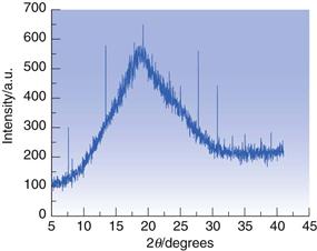
Fig. 23.15 XRPD diffractogram for amorphous trehalose.
Powder properties
Manufacturing processes frequently involve the movement, blending, manipulation and compression of powders and so will be affected by powder properties. Powder properties that are affected by size and shape can be manipulated without changing physical form by changing crystal habit.
Particle size and shape
Particle shape is most easily determined by visual inspection with a microscope (some typical particle shapes are shown in Fig. 23.16). Usually a light microscope will suffice, unless the material is a spray-dried or micronized powder, in which case scanning electron microscopy (SEM) might be a better option. If the particles are not spherical but are irregularly shaped, it is difficult to define exactly which dimension should be used to define the particle size. Several semi-empirical measures have been proposed, e.g. Feret’s diameter and Martin’s diameter (see Chapter 9, Fig. 9.3 and associated text).
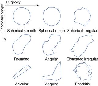
Fig. 23.16 Some typical powder shapes.
Powder flow
Powders must have good flow properties in order to fill tablet presses or capsule filling machines and to ensure blend uniformity when mixed with excipients. This is discussed in Chapter 12.
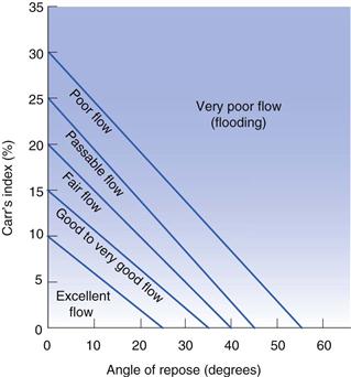
While poor powder flow will not hinder development of a dosage form it may prove a major challenge for commercial manufacture and so early assessment of powder flow allows time to ameliorate any problems. Assessing powder flow is easy when large volumes of material are available, but during preformulation methods must be used that require only small volumes of powder. The two most relevant methods of assessment at the preformulation stage involve the measurement of the angle of repose and measurement of bulk density. These measurements and their use in powder flow prediction are discussed in Chapter 12. The parameters of angle of repose (Table 12.1 and Table 12.2), Carr’s index (Eqn 12.14, Table 12.3) and Hausner ratio (Eqn 12.13, Table 12.3) (the latter two are both calculated from measurements of bulk density) have proved to be the most useful in predicting bulk properties when only a small amount of test material is available (illustrated in Fig. 23.17).
Compaction properties
Compaction is a result of the compression and cohesion properties of a drug (Chapter 30). These properties are usually very poor for most drug powders, but tablets are rarely made from drug alone. Excipients are added which have good compaction properties. With low-dose drugs, the majority of the tablet comprises excipients and so the properties of the drug are less important. However, once the dose increases above 50 mg the compaction characteristics of the drug will greatly influence the overall properties of the tablet.
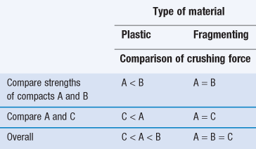
Information on the compaction properties of a drug candidate is very useful at the preformulation stage. A material to be tableted should preferably have plastic properties (i.e. once deformed it should remain deformed), but brittleness is also a beneficial characteristic, since the creation of fresh surfaces during fragmentation facilitates bond formation. Water content may also be important, since water frequently acts as a plasticizer, altering mechanical properties. A useful practical guide is that if a high dose drug behaves plastically, the excipients should fragment. Otherwise the excipients should deform plastically.
It is possible to assess the mechanical properties of a drug candidate even when only a small amount of material is available. One method (requiring compaction of only three tablets) is to follow the scheme suggested by Wells (1988).
4. Repeat with sample B, but hold the load at 1 tonne for 30 seconds before releasing the pressure.
Interpretation of the results is given in Table 23.14. This simple test will yield a significant amount of information on the possible commercial tabletability of a drug candidate from very little material.
Summary
Preformulation studies have a significant part to play in anticipating formulation problems and identifying logical development paths for both liquid and solid dosage forms. The need for adequate drug solubility cannot be overemphasized. The availability of good solubility data should allow the selection of the most appropriate salt for development. DSC and XRPD data will define physical form and indicate relative stability.
By comparing the physicochemical properties of each drug candidate within a therapeutic group, the preformulation scientist can assist the synthetic chemist to identify the optimum molecule, provide the biologist with suitable vehicles to elicit pharmacological response and advise the bulk chemist about the selection and production of the best salt with appropriate particle size and morphology for subsequent processing.
References
1. Kramer SF, Flynn GL. Solubility of organic hydrochlorides. Journal of Pharmaceutical Sciences. 1972;61:1896–1904.
2. Manallack DT. The pKa distribution of drugs: Application to drug discovery. Perspectives in Medicinal Chemistry. 2007;1:25–38.
3. Mota FL, Carneiro AP, Queimada AJ, Pinho SP, Macedo EA. Temperature and solvent effects in the solubility of some pharmaceutical compounds: measurements and modeling. European Journal of Pharmaceutical Sciences. 2009;37:499–507.
4. Nelson E. Solution rate of theophylline salts and effects from oral administration. Journal of the American Pharmaceutical Society (Scientific edition). 1957;46:607–614.
5. Sarveiya V, Templeton JF, Benson HAE. Ion-pairs of ibuprofen: Increased membrane diffusion. Journal of Pharmacy and Pharmacology. 2004;56:717–724.
6. Serajuddin ATM, Jarowski CI. Effect of diffusion layer pH and solubility on the dissolution rate of pharmaceutical acids and their sodium salts II: Salicylic acid, theophylline and benzoic acid. Journal of Pharmaceutical Sciences. 1985;74:148–154.
7. Stahl PH, Wermuth CG, eds. Handbook of Pharmaceutical Salts Properties, Selection and Use. 2nd edn Weinheim: Wiley-VCH; 2011.
8. Stephenson GA, Aburub A, Woods TA. Physical stability of weak bases in the solid-state. Journal of Pharmaceutical Sciences. 2011;100:1607–1617.
9. Wells JI. Pharmaceutical Preformulation The Physicochemical Properties of Drug Substances. Chichester: John Wiley and Sons; 1988.
Bibliography
1. Biagi GL, Barbaro AM, Sapone A, Recanatini M. Determination of lipophilicity by means of reversed-phase thin-layer chromatography i Basic aspects and relationship between slope and intercept of TLC equations. Journal of Chromatography A. 1994;662:341–361.
2. Bird AE, Marshall AC. Revered-phase thin layer chromatography and partition coefficients of penicillins. Journal of Chromatography A. 1971;63:313–319.
3. Bogardus JB, Blackwood RK. Solubility of doxycycline in aqueous solution. Journal of Pharmaceutical Sciences. 1979;68:188–194.
4. Brittain HG. Strategy for the prediction and selection of drug substance salt forms. Pharmaceutical Technology. 2007;31:78–88.
5. Brittain HG. Introduction and overview to the preformulation development of solid dosage forms. In: Adeyeye MC, Brittain HG, eds. Preformulation in Solid Dosage Form Development. New York: Informa Healthcare; 2008.
6. Carr RL. Evaluating flow properties of solids. Chemical Engineering. 1965;72:163–167.
7. Gaisford S, Saunders M. Essentials of Pharmaceutical Preformulation. Oxford: Wiley-Blackwell; 2013.
8. Govindarajan R, Zinchuk A, Hancock B, Shalaev E, Suryanarayanan R. Ionization states in the microenvironment of solid dosage forms: effect of formulation variables and processing. Pharmaceutical Research. 2006;23:2454–2468.
9. Li S, Doyle P, Metz S, Royce AE, Serajuddin ATM. Effect of chloride ion on dissolution of different salt forms of haloperidol, a model basic drug. Journal of Pharmaceutical Sciences. 2005;94:2224–2231.
10. Rowe RC, Sheskey PJ, Cook WG, Fenton ME. Handbook of Pharmaceutical Excipients. 7th edn London: The Pharmaceutical Press; 2012.
11. Valkó K. Application of high-performance liquid chromatography based measurements of lipophilicity to model biological distribution. Journal of Chromatography A. 2004;1037:299–310.
12. Weber Jr WJ, Chin Y-P, Rice CP. Determination of partition coefficients and aqueous solubilities by reverse phase chromatography – I Theory and background. Water Research. 1986;20:1433–1442.
13. Zannou EA, Yatindra QJ, Joshi M, Serajuddin ATM. Stabilization of the maleate salt of a basic drug by adjustment of microenvironment pH in solid dosage form. International Journal of Pharmaceutics. 2007;337:210–218.