Particle size analysis
John N. Staniforth and Kevin M.G. Taylor
Chapter contents
Particle size analysis methods
Electrical sensing zone method (Coulter Counter®)
Laser diffraction (low angle laser light scattering)
Photon correlation spectroscopy (dynamic light scattering)
Key points
Introduction
The size of particulate solids is important in achieving optimum formulation and production of efficacious medicines. Figure 9.1 shows an outline of the lifetime of a drug. During stages 1 and 2, when a drug is synthesized and formulated, the particle size of the drug and other powders in the formulation is determined, and this influences the physical performance of the medicine and the subsequent pharmacological effects of the drug.
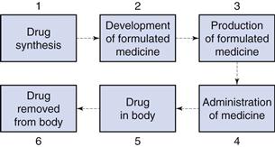
Particle size influences the production of many formulated medicines (stage 3, Fig. 9.1) as discussed in later chapters of this book. For instance, both tablets and capsules are manufactured using equipment that controls the mass of drug (and other solid excipients) by volumetric filling. Therefore, any interference with the uniformity of fill volumes may alter the mass of drug incorporated into the tablet or capsule and hence adversely affect the content uniformity of the medicine. Powders with different particle sizes have different flow and packing properties, which alter the volumes of powder during each encapsulation or tablet compression event. In order to avoid such problems, the particle sizes of drugs and other powders may be defined during formulation so that problems during production are avoided.
Following administration of the medicine (stage 4, Fig. 9.1), the dosage form should release the drug into solution at the optimum rate. This depends on several factors, one of which will be the particle size of drug, which is inversely related to particle size as described by the Noyes and Whitney equation, outlined in detail in Chapter 2. Thus, reducing the size of particles will generally increase the rate of dissolution, which can have a direct impact on bioavailability and subsequent drug handling by the body (stages 5 and 6). For example, the drug griseofulvin has a low solubility by oral administration, but is rapidly distributed following absorption; reducing the particle size increases the rate of dissolution and consequently the amount of drug absorbed. However, a reduction in particle size to improve dissolution rate and hence bioavailability is not always beneficial. For example, reducing the particle size of nitrofurantoin increases its dissolution rate, and may consequently produce adverse side-effects because of its more rapid absorption. The effect of particle size on bioavailability is discussed more fully in Chapter 20.
It is clear from the lifetime of a drug outlined above that the knowledge and control of particle size are of importance for both the production of medicines containing particulate solids and the efficacy of such medicines following administration.
The pharmaceutical scientist may not necessarily need to know the precise size of particles intended for a particular purpose, rather a size range may be specified, and consequently powders are frequently graded based on the size of the particles of which they are comprised. For instance:
Pharmacopoeial definitions of grades of powders, and the methods employed to separate particles, by size, are discussed in detail in Chapter 10.
Whilst this chapter refers to ‘particle size’ and ‘particle size analysis’ and the above discussion relates to solid particles, it should be noted that many of the concepts discussed in this chapter apply equally to pharmaceutical systems where it is necessary to determine the size of a dispersed liquid, rather than solid phase, for instance in emulsions and aerosol sprays.
Particle size
Dimensions
Describing the size of irregularly shaped particles, as usually encountered in pharmaceutical systems, is a challenge. To adequately describe such a particle would require measurement of no fewer than three dimensions. Frequently, though, it is advantageous to have a single number to describe the size of particles. For instance, when milling powders for inclusion in a pharmaceutical formulation, production and quality assurance staff will want to know if the mean size is approximately the same, larger or smaller than for previous milling procedures of the same material. To overcome the problem of describing a three-dimensional particle with a single number, we employ the concept of the equivalent sphere. Using this approach, a particle is considered to approximate to a sphere: some property of the particle is measured and related to a sphere, the diameter of which can be quoted. Because the measurement is then based on a hypothetical sphere, which represents only an approximation to the true size and shape of the particle, the dimension is referred to as the equivalent sphere diameter or equivalent diameter of the particle.
Equivalent sphere diameters
It is possible to generate more than one sphere which is equivalent to a given irregular particle shape. Figure 9.2 shows the two-dimensional projection of a particle with two different diameters constructed about it.
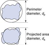
The projected area diameter is based on a circle of equivalent area to that of the projected image of a particle; the perimeter diameter is based on a circle having the same perimeter as the particle. Unless the particles are unsymmetrical in three dimensions then these two diameters will be independent of particle orientation.
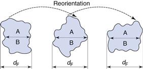
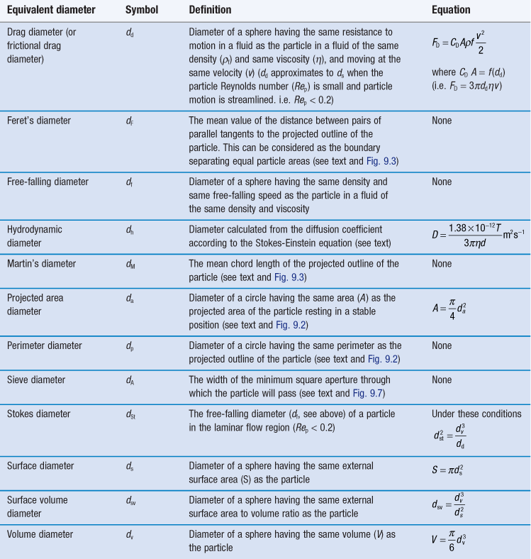
This is not true for Feret’s and Martin’s diameters (Fig. 9.3), the values of which are dependent on both the orientation and the shape of the particles. These are statistical diameters which are averaged over many different orientations to produce a mean value for each particle diameter. Feret’s diameter is determined from the mean distance between two parallel tangents to the projected outline of the particle. Martin’s diameter is the mean chord length of the projected particle perimeter, which can be considered as the boundary separating equal particle areas (A and B in Fig. 9.3).
It is also possible to determine the equivalent sphere diameters of particles based on other factors such as volume, surface, sieve aperture, sedimentation characteristics, etc. Some of the more commonly used equivalent sphere diameters are defined in Table 9.1; there are others. In general, the method used to determine particle size dictates the type of equivalent diameter that is measured. This is explained for each particle size analysis method described later in this chapter. Inter-conversion of the various equivalent particle sizes may be carried out and this can be done mathematically or automatically as part of the size analysis.
Particle size distribution
A particle population which consists of spheres or equivalent spheres of the same diameter is said to be monodispersed or monosized, and its characteristics can be described by a single diameter or equivalent sphere diameter.
However, it is unusual for particles to be completely monodispersed and such a sample will rarely, if ever, be encountered in a pharmaceutical system. Most powders contain particles with a range of different equivalent diameters, i.e. they are polydispersed or heterodispersed. In order to be able to define a size distribution or compare the characteristics of two or more powders consisting of particles with many different diameters, the size distribution can be broken down into different size ranges, which can be presented in the form of a histogram plotted from data such as those in Table 9.2.
Table 9.2
Frequency and cumulative frequency distribution data for a nominal particle size analysis procedure
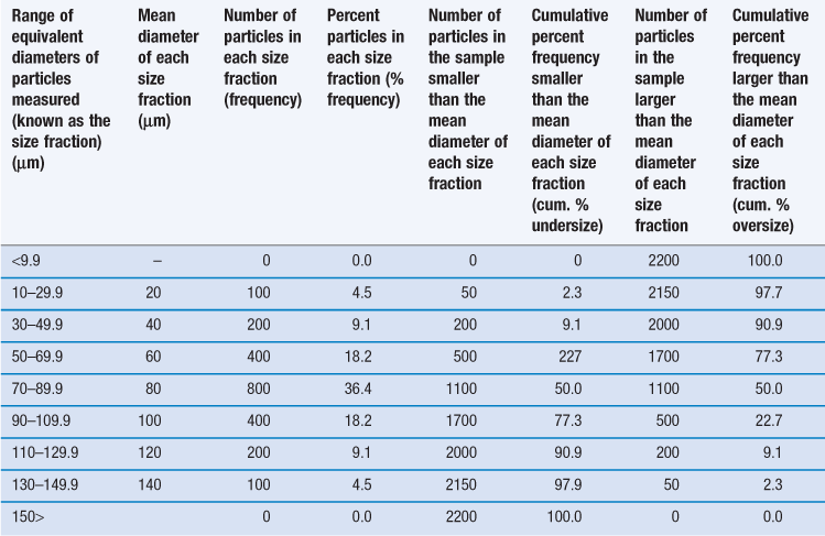
Such a histogram presents an interpretation of the particle size distribution and enables the percentage of particles having a given equivalent diameter to be determined. A histogram allows different particle size distributions to be compared. For example, the histogram in Figure 9.4a is a representation of particles that are normally distributed symmetrically about a central value. The peak frequency value, known as the mode, separates the normal curve into two identical halves, because the size distribution is fully symmetrical, i.e. the data in Table 9.2 are normally distributed.
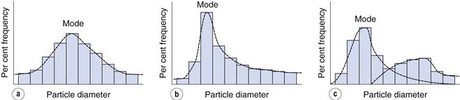
Not all particle populations are characterized by symmetrical, or normal, size distributions and the frequency distributions of such populations are said to be skewed. The size distribution shown in Figure 9.4b contains a large proportion of fine particles. A frequency curve such as this, with an elongated tail towards higher size ranges is said to be positively skewed; the reverse case exhibits negative skewness. These skewed distributions can sometimes be normalized by replotting the equivalent particle diameters using a logarithmic scale, and are thus usually referred to as log-normal distributions.
In some size distributions more than one mode occurs: Figure 9.4c shows a bimodal frequency distribution for a powder which has been subjected to milling. Some of the coarser particles from the unmilled population remain unbroken and produce a mode towards the highest particle size, whereas the fractured (size reduced) particles have a new mode which appears lower down the size range.
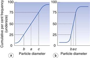
An alternative to the histogram representation of particle size distribution is obtained by sequentially adding the percent frequency values, as shown in Table 9.2, to produce a cumulative percent frequency distribution. If the addition sequence begins with the coarsest particles, the values obtained will be cumulative percent frequency undersize (or more commonly cumulative percent undersize); the reverse case produces a cumulative percent oversize.
It is possible to compare two or more particle populations using the cumulative distribution representation. Figure 9.5 shows two cumulative percent frequency distributions. For example, the size distribution in Figure 9.5a shows that this powder has a larger range or spread of diameters than the powder represented in Figure 9.5b. The median particle diameter corresponds to the point that separates the cumulative frequency curve into two equal halves, above and below which 50% of the particles lie (point a in Fig. 9.5). Just as the median divides a symmetrical cumulative size distribution curve into two equal halves, so the lower and upper quartile points at 25% and 75% divide the upper and lower ranges of a symmetrical curve into equal parts (points b and c, respectively, in Fig. 9.5).
Statistical methods to summarize size distribution data
Although it is possible to describe particle size distributions qualitatively, it is always more satisfactory to compare particle size data quantitatively. This is made possible by summarizing the distributions using statistical methods.
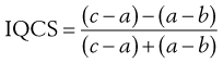
In order to quantify the degree of skewness of a particle population, the interquartile coefficient of skewness (IQCS) can be determined as follows:
 (9.1)
(9.1)
where a is the median diameter and b and c are the lower and upper quartile points (see Fig. 9.5).
The IQCS can take any value between −1 and +1. If the IQCS is zero then the size distribution is practically symmetrical between the quartile points. To avoid ambiguity in interpreting values for IQCS, a large number of size intervals is required.
To quantify the degree of symmetry of a particle size distribution, a property known as kurtosis can be determined. The symmetry of a distribution is based on a comparison of the height or thickness of the tails and the ‘sharpness’ of the peaks with those of a normal distribution. ‘Thick’-tailed, ‘sharp’ peaked curves are described as leptokurtic, whereas ‘thin’-tailed, ‘blunt’ peaked curves are platykurtic and the normal distribution is mesokurtic.
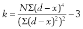
The coefficient of kurtosis, k (Eqn 9.2), has a value of 0 for a normal curve, a negative value for curves showing platykurtosis and positive values for leptokurtic size distributions:
 (9.2)
(9.2)
where d is any particle diameter, x is mean particle diameter and N is number of particles. Again, a large number of data points is required to provide an accurate analysis.
Mean particle sizes
As established above, it is impossible for any single number to fully describe the size distribution of particles in a real pharmaceutical system. However, for the sake of simplicity, pharmaceutical scientists wish to employ a single number to represent the mean size of a powder sample. The mean of the particle population, the median (Fig. 9.5) and the mode (Fig. 9.4) are all measures of central tendency. They provide a single value near the middle of the size distribution that attempts to represent a central particle diameter. Whereas the mode and median diameters can be obtained for an incomplete particle size distribution, the mean diameter can only be determined when the size distribution is complete and the upper and lower size limits are known. It is possible to define the ‘mean’ particle size in several ways.
Arithmetic means
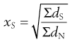
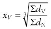
Arithmetic means are obtained by summating a particular parameter for all the individual particles in a sample and dividing the value achieved by the total number of particles. Means can be related to the diameter, surface area, volume or mass of a particle. In the equations below, x is the mean particle size and the subscripts L, S, V and M indicate mean size based on length (diameter), surface area, volume and mass, respectively. ΣdL is the sum of the diameters of all the particles, etc., and ΣdN is the total number of particles in the sample.
 (9.3)
(9.3)
 (9.4)
(9.4)
 (9.5)
(9.5)
 (9.6)
(9.6)
Such means are strictly referred to as number mean or number average particle sizes as they are based on the number of particles. Equivalent sets of equations exist based on, for example, the mass of individual particles, giving mass mean or mass average particle size. In this case the two types of mean will differ as numerous small particles contribute little to the mass (mass being related to radius3). Consequently, number average particle sizes are smaller than the equivalent mass average sizes.
Geometric means
As explained above, not all powder samples show an arithmetic distribution of particle sizes; some (particularly after milling) follow a log-normal distribution. In a log-normal distribution the frequency, f, of the occurrence of any given particle of equivalent diameter d is given by:
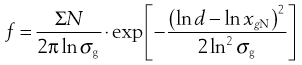 (9.7)
(9.7)
where xgN is the number geometric mean diameter and σg is the geometric standard deviation.
Interconversion of mean sizes
For powders exhibiting a log-normal distribution of particle size, a series of relationships, sometimes known as the Hatch–Choate equations, links the different mean diameters of a size distribution. There are numerous combinations of these and the interested reader is referred to Allen (1997) for further details.
Influence of particle shape
The techniques discussed above for representing particle size distribution are all based on the assumption that particles can be adequately represented by an equivalent circle or sphere. Whilst this is often the case, in some pharmaceutically relevant cases, particles deviate markedly from circularity and sphericity, and the use of a single equivalent diameter measurement may be inappropriate. For example, a powder consisting of monosized fibrous particles would appear to have a wide size distribution according to statistical diameter measurements. However, the use of an equivalent diameter based on projected area would also be misleading. Under such circumstances it may be desirable to return to the concept of characterizing a particle using more than one dimension. Thus, the breadth of the fibre could be obtained using a projected circle inscribed within the fibre (di) and the fibre length could be measured using a projected circle circumscribed around the fibre dc (Fig. 9.6).
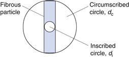
The ratio of inscribed circle to circumscribed circle diameters can also be used as a simple shape factor to provide information about the circularity of a particle. The ratio di/dc will be 1 for a circle and diminish as the particle becomes more acicular.
Such comparisons of equivalent sphere diameters determined by different methods offer considerable scope for both particle size and particle shape analysis. For example, measurement of particle size to obtain a projected area diameter, da, and an equivalent volume diameter, dv, provides information concerning the surface area : volume ratio or bulkiness of a group of particles, which can also be useful in interpreting particle size data.
Particle size analysis methods
In order to obtain equivalent sphere diameters with which to characterize the particle size of a powder, it is necessary to carry out a size analysis using one or more different methods. Particle size analysis methods can be divided into different categories based on several different criteria: size range of analysis; wet or dry methods; manual or automatic methods or speed of analysis. Note that the specialist area of sizing aerosolized particles using cascade impactor techniques is described in Chapter 37. Particle size instrumentation is developing quickly, but a summary of the principles of these different methods is presented below, based on the salient features of each technique.
Sieve methods
Equivalent diameter
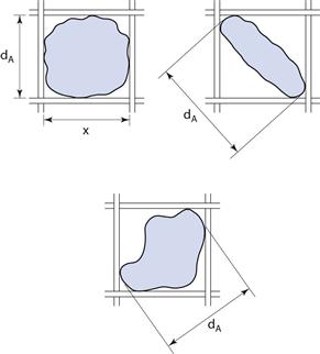
Sieve diameter, dA, as defined in Table 9.1 and shown diagrammatically in Figure 9.7 for different-shaped particles.
Range of analysis
The International Standards Organization (ISO) sets a lowest sieve diameter of 45 µm and, as powders are usually defined as having a maximum diameter of 1000 µm, this could be considered to be the upper limit. In practice, sieves can be obtained for size analysis over a range from 5 to 125 000 µm. These ranges are shown diagrammatically in Figure 9.8.
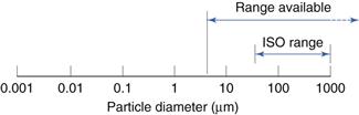
Fig. 9.8 Size range of analysis using sieves.
Sample preparation and analysis conditions
Sieve analysis is usually carried out using dry powders, although for powders in liquid suspension or which agglomerate during dry sieving, a process of wet sieving can be used.
Principles of measurement
Sieve analysis utilizes a woven, punched or electroformed mesh, often in brass or stainless steel, with known aperture diameters which forms a physical barrier to particles. Most sieve analyses use a series, stack or ‘nest’ of sieves, which has the smallest mesh above a collector tray followed by meshes that become progressively coarser towards the top of the stack of sieves. A sieve stack usually comprises 6–8 sieves with an aperture progression based on a  or
or  change in diameter between adjacent sieves. Powder is loaded on to the coarsest sieve at the top of the assembled stack and the nest is subjected to mechanical vibration. After a suitable time the particles are considered to be retained on the sieve mesh with an aperture corresponding to the sieve diameter. Sieving is rarely complete as some particles can take a long time to orientate themselves over the sieve apertures and pass through. Thus sieving times should not be arbitrary, and it is recommended that sieving be continued until less than 0.2% of material passes a given sieve aperture in any 5-minute interval.
Alternative techniques
Another form of sieve analysis, called air-jet sieving, uses individual sieves rather than a complete nest of sieves. Starting with the finest-aperture sieve and progressively removing the undersize particle fraction by sequentially increasing the apertures of each sieve, particles are encouraged to pass through each aperture under the influence of a partial vacuum applied below the sieve mesh. A reverse air-jet circulates beneath the sieve mesh, blowing oversize particles away from the mesh to prevent blocking. Air-jet sieving is often more efficient and reproducible than using mechanically vibrated sieve analysis, although with finer particles, agglomeration can become a problem.
Automatic methods
Sieve analysis is still largely a non-automated process, although an automated wet sieving technique has been described.
Microscope methods
Equivalent diameters
Projected area diameter, da; perimeter diameter, dp; Feret’s diameter, dF and Martin’s diameter, dM (all defined in Table 9.1).
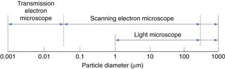
Range of analysis
This is shown diagrammatically in Figure 9.9.
Sample preparation and analysis conditions
Specimens prepared for light microscopy must be adequately dispersed on a microscope slide to avoid analysis of agglomerated particles. Specimens for scanning electron microscopy are prepared by fixing to aluminium stubs before sputter coating with a film of gold a few nanometres in thickness. Specimens for transmission electron microscopy are often set in resin, sectioned by microtome and supported on a metal grid before metallic coating.
Principles of measurement
Size analysis by light microscopy is carried out on two-dimensional images of particles which are generally assumed to be randomly oriented in three dimensions. In many cases, this assumption is valid, although for dendrites, fibres or flakes it is very improbable that the particles will orient with their minimum dimensions in the plane of measurement. Under such conditions, size analysis is carried out accepting that they are viewed in their most stable orientation. This will lead to an overestimation of size, as the largest dimensions of the particle will be observed as the smallest dimension will most often orientate vertically.
The two-dimensional images are analysed according to the desired equivalent diameter. Using a conventional light microscope, particle size analysis can be carried out using a projection screen with screen distances related to particle dimensions by a previously derived calibration factor using a graticule. A graticule can also be used which has a series of opaque and transparent circles of different diameters, usually in a  progression. Particles are compared with the two sets of circles and are sized according to the circle that corresponds most closely to the equivalent particle diameter being measured. The field of view is divided into segments to facilitate measurement of different numbers of particles.
Alternative techniques
Alternatives to light microscopy include scanning electron microscopy (SEM) and transmission electron microscopy (TEM). SEM is particularly appropriate when a 3-dimensional particle image is required; in addition, the very much greater depth of field of an SEM compared to a light microscope may also be beneficial. Both SEM and TEM analysis allow the lower particle sizing limit to be greatly extended over that possible with a light microscope.
Automatic methods
Semi-automatic methods of microscope analysis use some form of precalibrated variable distance to split particles into different size ranges. One technique, called a particle comparator, utilizes a variable-diameter light spot projected on to a photomicrograph or electron photomicrograph of a particle under analysis. The variable iris controlling the light spot diameter is linked electronically to a series of counter memories, each corresponding to a different size range (Fig. 9.10). Alteration of the iris diameter causes the particle count to be directed into the appropriate counter memory following activation of a switch by the operator.
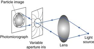
Fig 9.10 Particle comparator.
A second technique uses a double-prism arrangement mounted in place of the light microscope eyepiece. The image from the prisms is usually displayed on a video monitor. The double-prism arrangement allows light to pass through to the monitor unaltered, where the usual single particle image is produced. When the prisms are sheared against one another, a double image of each particle is produced and the separation of the split images corresponds to the degree of shear between the prisms (Fig. 9.11). Particle size analysis can be carried out by shearing the prisms until the two images of a single particle make touching contact. The prism-shearing mechanism is linked to a precalibrated micrometer scale from which the equivalent diameter can be read directly. Alternatively, a complete size distribution can be obtained more quickly by subjecting the prisms to a sequentially increased and decreased shear distance between two preset levels corresponding to a known size range. All particles whose images separate and overlap sequentially under a given shear range are considered to fall in this size range, and are counted by operating a switch which activates the appropriate counter memory. Particles whose images do not overlap in either shear sequence are undersize and particles whose images do not separate in either shear mode are oversize and will be counted in a higher size range.
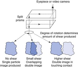
Fig 9.11 Image-shearing eyepiece.
Fully automated image analysis has the advantage of being more objective and very much faster, and also enables a much wider variety of size and shape parameters to be processed. Image acquisition is usually achieved by digital imaging, with a CCD sensor placed in the optical path of the microscope to generate high resolution images. This allows both image analysis and image processing to be carried out.
Sedimentation methods
Equivalent diameters
(Frictional) drag diameter, dd, and Stokes diameter, dSt (Table 9.1).
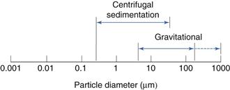
Range of analysis
This is shown diagrammatically in Figure 9.12.
Sample preparation and analysis conditions
Particle size distributions can be determined by examining the powder as it sediments. In cases where the powder is not uniformly dispersed in a fluid, it can be introduced as a thin layer on the surface of the liquid. If the powder is hydrophobic it may be necessary to add a dispersing agent to aid wetting. In cases where the powder is soluble in water, it will be necessary to use non-aqueous liquids or carry out the analysis in a gas.
Principles of measurement
Techniques of size analysis by sedimentation can be divided into two main categories according to the method of measurement used. One type is based on the measurement of particles in a retention zone; a second type uses a non-retention measurement zone.
An example of a non-retention zone measurement method is known as the pipette method. In this method, known volumes of suspension are drawn off and the concentration differences are measured with respect to time.
One of the most popular of the pipette methods was that developed by Andreasen and Lundberg and is commonly called the Andreasen pipette (Fig. 9.13). The Andreasen fixed-position pipette consists of a graduated cylinder which can hold approximately 500 mL of suspension fluid. A pipette is located centrally in the cylinder and is held in position by a ground-glass stopper so that its tip coincides with the zero level. A three-way tap allows fluid to be drawn into a 10 mL reservoir, which can then be emptied into a beaker or centrifuge tube. The amount of powder can be determined by weight following drying or centrifuging; alternatively, chemical analysis of the particles can be carried out.
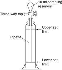
Fig 9.13 Diagram of Andreasen pipette.
The largest size present in each sample is then calculated from Stokes’ equation. Stokes’ Law is an expression of the drag factor in a fluid and is linked to the flow conditions characterized by a Reynolds number. Drag is one of three forces acting on a particle sedimenting in a gravitational field. A drag force, Fd, acts upwards, as does a buoyancy force, Fb; a third force is gravity, Fg, which acts as the driving force of sedimentation. At the constant terminal velocity, which is rapidly achieved by sedimenting particles, the drag force becomes synonymous with particle motion. Thus for a sphere of diameter d and density ρs, falling in a fluid of density ρf, the equation of motion is:
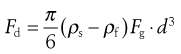 (9.8)
(9.8)
According to Stokes:
 (9.9)
(9.9)
where vSt is the Stokes terminal velocity, i.e. sedimentation rate. That is:
 (9.10)
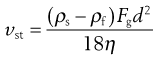
as vSt = h/t where h is sedimentation height or distance and t is sedimentation time. By rearrangement, Stokes’ equation is obtained:
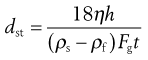 (9.11)
Stokes’ equation for determining particle diameters is based on the following assumptions:
• motion equivalent to that in a fluid of infinite length
• terminal velocity conditions
• low settling velocity so that inertia is negligible
• large particle size relative to fluid molecular size, so that diffusion is negligible
The second type of sedimentation size analysis, using retention zone methods, also uses Stokes’ Law to quantify particle size. One of the most common retention zone methods uses a sedimentation balance. In this method the amount of sedimented particles falling on to a balance pan suspended in the fluid is recorded. The continual increase in weight of sediment is recorded with respect to time.
Alternative techniques
One of the limitations of gravitational sedimentation is that below a diameter of approximately 5 µm, particle settling becomes prolonged and is subject to interference from convection, diffusion and Brownian motion. These effects can be minimized by increasing the driving force of sedimentation by replacing gravitational forces with a larger centrifugal force. Once again, sedimentation can be monitored by retention or non-retention methods, although the Stokes’ equation requires modification because particles are subjected to different forces according to their distance from the axis of rotation. To minimize the effect of distance on the sedimenting force, a two-layer fluid system can be used. A small quantity of concentrated suspension is introduced on to the surface of a bulk sedimentation liquid known as spin fluid. Using this technique of disc centrifugation, all particles of the same size are in the same position in the centrifugal field and hence move with the same velocity.
Automatic methods
In general, gravity sedimentation methods tend to be less automated than those using centrifugal forces. However, an adaptation of a retention zone gravity sedimentation method is known as a micromerograph and measures sedimentation of particles in a gas rather than a fluid. The advantages of this method are that sizing is carried out relatively rapidly and the analysis is virtually automatic.
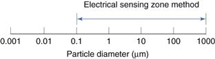
Electrical sensing zone method (Coulter Counter®)
Equivalent diameter
Volume diameter, dv (Table 9.1).
Range of analysis
This is shown diagrammatically in Figure 9.14.
Sample preparation and analysis conditions
Powder samples are dispersed in an electrolyte to form a very dilute suspension, which is usually subjected to ultrasonic agitation for a period to break up any particle aggregates. A dispersant may also be added to aid particle deaggregation.
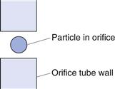
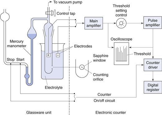
Principles of measurement
The particle suspension is drawn through an aperture/orifice (Fig. 9.15) accurately drilled through a sapphire crystal set into the wall of a hollow glass tube. Electrodes, which are situated on either side of the aperture and surrounded by an electrolyte solution, monitor the change in electrical signal that occurs when a particle momentarily occupies the orifice and displaces its own volume of electrolyte. The volume of suspension drawn through the orifice is determined by the suction potential created by mercury rebalancing in a convoluted U-tube (Fig. 9.16). The volume of electrolyte fluid which is displaced in the orifice by the presence of a particle causes a change in electrical resistance between the electrodes that is proportional to the volume of the particle. The change in resistance is converted into a voltage pulse which is amplified and processed electronically. Pulses falling within precalibrated limits or thresholds are used to split the particle size distribution into many different size ranges. In order to carry out size analysis over a wide diameter range, it will be necessary to change the orifice diameter (and hence tube) used, to prevent coarser particles blocking a small-diameter orifice. Conversely, finer particles in a large-diameter orifice will cause too small a relative change in volume to be accurately quantified. Dispersions must be sufficiently dilute to avoid the occurrence of coincidence, whereby more than one particle may be present in the orifice at any one time. This may result in a loss of count (i.e. two particles counted as one) and inaccurate measurement as the equivalent sphere diameter is based on the volume of two particles, rather than one.
Alternative techniques
Since the electrical sensing zone method principle was first described, there have been some modifications to the basic method, such as the use of alternative orifice designs and hydrodynamic focusing, but in general the particle sizing technique remains the same.
Another type of stream sensing analyser utilizes the attenuation of a light beam by particles drawn through the sensing zone. Some instruments of this type use the change in reflectance, whereas others use the change in transmittance of light. It is also possible to use ultrasonic waves generated and monitored by a piezoelectric crystal at the base of a flow-through tube containing particles in fluid suspension.
Laser diffraction (low angle laser light scattering)
Equivalent diameters
Projected area diameter, da, and, following computation, volume diameter, dv (both defined in Table 9.1).
Range of analysis
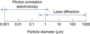
This is shown diagrammatically in Figure 9.17.
Sample preparation and analysis conditions
Depending on the type of measurement to be carried out and the instrument used, particles can be presented dispersed in either liquid or air.
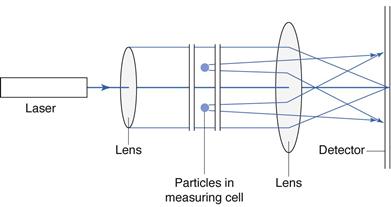
Principles of measurement
Moncohromatic light from a helium-neon laser is incident on the sample of particles and diffraction occurs. The scattered light is focused by a lens directly on to a photodetector, comprising a series of detectors (Fig. 9.18). The light flux signals occurring on the photodetector are converted into electrical current, which is digitized and processed into size distribution data, based on the principles of Fraunhofer diffraction or Mie theory.
Fraunhofer diffraction and Mie theory
For particles that are much larger than the wavelength of light, any interaction with particles causes light to be scattered in a forward direction with only a small change in angle. This phenomenon is known as Fraunhofer diffraction and produces light intensity patterns that occur at regular angular intervals, with the angle of scatter inversely proportional to the particle diameter producing it. The composite diffraction pattern produced by different diameter particles may be considered to be the sum of all the individual patterns produced by each particle in the size distribution, at low to medium particle concentrations.
As the size of particles approaches the dimension of the wavelength of the light, some light is still scattered in the forward direction, according to Mie scatter theory, but there is also some side scatter at different wavelengths and polarizations. Use of the Mie theory requires consideration of the optical properties of the dispersed particles and the dispersion medium, i.e. knowledge of their respective refractive indices is required for calculation of particle size distributions.
Alternative techniques
There is a wide variety of different instruments based on laser Doppler anemometry or velocimetry and diffraction measurements.
Automatic methods
Most of the instruments based on laser diffraction produce a full particle size analysis automatically, with data are presented in graphical and tabular form.
Photon correlation spectroscopy (dynamic light scattering)
Equivalent diameters
Hydrodynamic diameter, dh, defined in Table 9.1.
Range of analysis
This is shown diagrammatically in Figure 9.17.
Sample preparation and analysis conditions
Particles are presented in liquid suspension.
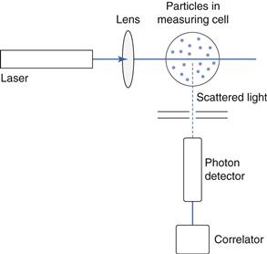
Principles of measurement
In photon correlation spectroscopy (PCS), also called dynamic light scattering (DLS) and quasi-elastic light scattering (QELS), the intensity of scattered light at a given angle is measured as a function of time for a population of particles. The rate of change of the scattered light intensity is a function of the movement of the particles by Brownian motion. Brownian motion is the random movement of a small particle or macromolecule caused by collisions with the smaller molecules of the suspending fluid. It is independent of external variations, except the viscosity of the suspending fluid and its temperature, and as it randomizes particle orientations, any effects of particle shape are minimized. Brownian motion is independent of the suspending medium and although increasing the viscosity does slow down the motion, the amplitude of the movements is unaltered. Because the suspended small particles are always in a state of motion, they undergo diffusion. Diffusion is governed by the mean free path of a molecule or particle, which is the average distance of travel before diversion by collision with another molecule. PCS analyses the constantly changing patterns of laser light scattered or diffracted by particles undergoing Brownian motion, and monitors the rate of change of scattered light during diffusion. In most instruments, monochromatic light from a helium-neon laser is focused onto the measurement zone, containing particles dispersed in a liquid medium (Fig 9.19). Light is scattered at all angles, and is often detected using a detector placed at an angle of 90°. The detection and spatial resolution of the fluctuations in the intensity of the scattered light, is converted via a digital correlator into size distribution data.
Brownian diffusion causes a three-dimensional random movement of particles, where the mean distance travelled,  , does not increase linearly with time, t, but according to the following relationship:
 (9.12)
where D is the diffusion coefficient.
A basic property of molecular kinetics is that each particle or macromolecule has the same average thermal or kinetic energy, E, regardless of mass, size or shape:
 (9.13)
where k is Boltzmann’s constant and T is absolute temperature (Kelvin).
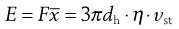
Thus at T = 0 K, molecules possess zero kinetic energy and therefore do not move. E can also be equated with the driving force, F, of particle motion:
 (9.14)
At equilibrium:
 (9.15)
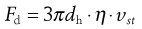
where Fd is the drag force resisting particle motion. According to Stokes’ theory, discussed above (Eqn 9.9):
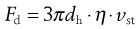 (9.16)
where dh is the hydrodynamic diameter, vst the Stokes velocity of the particle and η the fluid viscosity, i.e.:
 (9.17)
but
 (9.18)
and
 (9.19)
substituting,
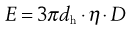 (9.20)
since E = kt (Eqn 9.13)
 (9.21)
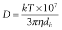
or
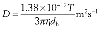 (9.22)
Equation 9.22, known as the Stokes–Einstein equation is the basis for calculation of particle diameters using PCS. This calculation assumes that particles are spherical, and a very low particle concentration is required. The technique determines the hydrodynamic diameter. As colloidal particles in a liquid dispersion have an adsorbed layer of ions/molecules from the dispersion medium that moves with the particles, hydrodynamic diameter is larger than the physical size of the particle (Merkus, 2009). Most instruments also yield a polydispersity index, determined by cumulant analysis as described in the International Standard on dynamic light scattering. The polydispersity index gives information regarding the width of the size distribution, with values ranging between 0 and 1.
Alternative techniques
The instruments vary according to their ability to characterize different particle size ranges, produce complete size distributions, measure dispersions of both solid and liquid particles, and determine molecular weights, diffusion coefficients, zeta potential or electrophoretic mobility.
Automatic methods
Most of the instruments based on laser light scattering produce a full particle size analysis automatically, with data presented in graphical and tabular forms.
Selection of a particle size analysis method
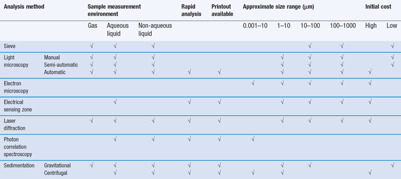
The selection of a particle size analysis method may be constrained by the instruments available in a laboratory, but wherever possible, the limitations on the choice of method should be governed by the properties of the sample being investigated and the type of size information required. For example, size analysis over a very wide range of particle diameters may preclude the use of a gravitational sedimentation method; alternatively, size analysis of aerosol particles would not be carried out using an electric sensing zone method. As a general guide, it is often most appropriate to determine the particle size distribution of a powder in an environment that most closely resembles the conditions in which the powder will be processed or handled. There are many different factors influencing the selection of an analysis method: these are summarized in Table 9.3 and these should be considered together with information from a preliminary microscopy analysis and any other known physical properties of the powder, such as solubility, density, cohesiveness, in addition to analysis requirements such as speed of measurement, particle size data processing or the physical separation of different particle size powders for subsequent processing.
References
1. Allen T. Particle Size Measurement. vols 1 and 2 5th edn London: Chapman and Hall; 1997.
2. Merkus HG. Particle Size Measurements: Fundamentals, Practice, Quality. New York: Springer; 2009.
Bibliography
1. Ahuja S, Scypinski S, eds. Handbook of Modern Pharmaceutical Analysis. 2nd edn Amsterdam: Academic Press; 2010.
2. Barnett MI, Nystrom C. Coulter counters and microscopes for the measurement of particles in the sieve range. Pharmaceutical Technology. 1982;6:49–50.
3. de Boer GBJ, de Weerd C, Thoenes D, Goosens HWJ. Laser Diffraction Spectrometry: Fraunhofer Diffraction Versus Mie Scattering. Particle & Particle Systems Characterization. 1987;4:14–19.
4. Kaye BH. Particle-size characterization. In: Swarbrick J, ed. Encyclopedia of Pharmaceutical Technology. 3rd edn New York: Informa Healthcare; 2006.
5. Manual on Test Sieving Methods. (ASTM Special Technical Publication). Pennsylvania: American Society for Testing and Materials Standards; 1985.
6. Masuda H, Higashitani K, Yoshida H, eds. Powder Technology Handbook. 3rd edn Boca Raton: CRC Press; 2006.
7. Rhodes M, ed. Principles of Powder Technology. Chichester: John Wiley; 1990.
8. Xu R. Particle Characterization: Light Scattering Methods (Particle Technology Series). New York: Springer; 2001.