Chapter 33A Neuroimaging
Structural Imaging: Magnetic Resonance Imaging, Computed Tomography
Computed Tomography
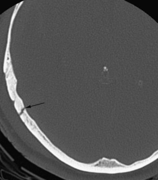
By changing the settings of the process of transforming the x-ray attenuation values to shades on the grayscale, it is possible to select which tissues to preferentially display in the image. This is referred to as windowing. Utilizing a bone window, for instance, is very useful for evaluating fractures in cases of craniofacial trauma (Fig. 33A.1).
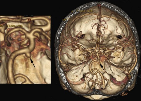
More than 20 years ago, a fast-imaging technique called spiral (or helical) CT scanning was introduced to clinical practice. With this technique, the x-ray tube in the gantry rotates continuously, but data acquisition is combined with continuous movement of the patient through the gantry. The circular rotating path of the x-rays, combined with the linear movement of the imaged body, results in a spiral or helix-shaped x-ray path, hence the name. These scanners can acquire data rapidly, and a large volume can be scanned in 20 to 60 seconds. This technique offers several advantages, including more rapid image acquisition. During the short scan time, patients can usually hold their breath, which reduces/minimizes motion artifacts. Timing of contrast bolus administration can be optimized, and less contrast material is sufficient. The short scan time, optimal contrast bolus timing, and better image quality are very useful in CT angiography, where cervical and intracranial blood vessels are visualized. These images can also be reformatted as 3D views of the vasculature, which are often displayed in color and can be depicted along with reformatted bone or other tissues in the region of interest (Fig. 33A.2).
Magnetic Resonance Imaging
Basic Principles
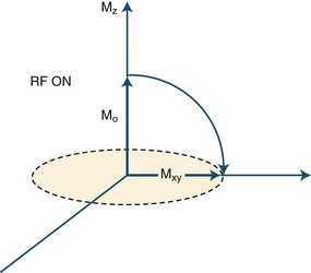
In clinical practice, MRI uses the magnetic characteristics inherent to the protons of hydrogen nuclei in the tissue, mostly in the form of water but to a significant extent in fat as well. The protons spin about their own axes, which creates a magnetic dipole moment for each proton (Fig. 33A.3). In the absence of an external magnetic field, the axes of these dipoles are arranged randomly, and therefore, the vectors depicting the dipole moments cancel each other out, resulting in a zero net magnetization vector and a zero net magnetic field for the tissue.

(A from Higgins, D., 2010. ReviseMRI. http://www.revisemri.com/questions/basicphysics/precession; B Reprinted with permission from Hashemi, R.H., Bradley, W.G., Lasanti, C.J., 2004. MRI—The Basics. 2nd ed. Lippincott Williams & Wilkins.)
This situation changes when the body is placed in the strong magnetic field of a scanner (see Fig. 33A.3, A). The magnetic field is generated by an electric current circulating in wire coils that surround the open bore of the scanner. Most MRI scanners used in clinical practice are superconducting magnets. Here the electrical coils are housed at near–absolute zero temperature, minimizing their resistance and allowing for the strong currents needed to generate the magnetic field without undue heating. The low temperature is achieved by cryogens (liquid nitrogen or helium). Most clinical scanners in commercial production today produce magnetic fields at strengths of 1.5 or 3.0 tesla (T).
When the patient is placed in the MRI scanner, the magnetic dipoles in the tissues line up relative to the external magnetic field. Some dipoles will point in the direction of the external field (“north”), some will point in the opposite direction (“south”), but the net magnetization vector of the dipoles (the sum of individual spins) will point in the direction of the external field (“north”), and this will be the tissue’s acquired net magnetization. At this point, a small proportion of the protons (and therefore the net magnetization vector of the tissue) is aligned along the external field (longitudinal magnetization), and the protons precess with a certain frequency. The term precession describes a proton spinning about its own axis and its simultaneous wobbling about the axis of the external field (see Fig. 33A.3, B). The frequency of precession is directly proportional to the strength of the applied external magnetic field.
As a next step in obtaining an image, a radiofrequency pulse is applied to the part of the body being imaged. This is an electromagnetic wave, and if its frequency matches the precession frequency of the protons, resonance occurs. Resonance is a very efficient way to give or receive energy. In this process, the protons receive the energy of the applied radiofrequency pulse. As a result, the protons flip, and the net magnetization vector of the tissue ceases transiently to be aligned with that of the external field but flips into another plane, thereby transverse magnetization is produced. One example of this is the 90-degree radiofrequency pulse that flips the entire net magnetization vector by 90 degrees to the transverse (horizontal) plane (Fig. 33A.4). What we detect in MRI is this transverse magnetization, and its degree will determine the signal intensity. Through the process of electromagnetic induction, rotating transverse magnetization in the tissue induces electrical currents in receiver coils, thus accomplishing signal detection. Several cycles of excitation pulses by the scanner with detection of the resulting electromagnetic signal from the imaged subject are repeated per imaged slice. This occurs while varying two additional magnetic field gradients along the x and y axes for each cycle. Varying the magnetic field gradient along these two additional axes, known as phase and frequency encoding, is necessary to obtain sufficient information to decode the spatial coordinates of the signal emitted by each tissue voxel. This is accomplished using a mathematical algorithm known as a Fourier transform. The final image is produced by applying a gray scale to the intensity values calculated by the Fourier transform for each voxel within the imaging plane, corresponding to the signal intensity of individual tissue elements.
T1 and T2 Relaxation Times
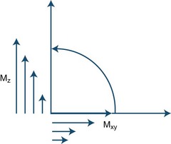
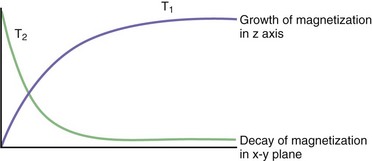
During the process of resonance, the applied 90-degree radiofrequency pulse flips the net magnetization vectors of the imaged tissues to the transverse (horizontal) plane by transmitting electromagnetic energy to the protons. The radiofrequency pulse is brief, and after it is turned off the magnitude of the net magnetization vector starts to decrease along the transverse or horizontal plane and return (“recover or relax”) toward its original position, in which it is aligned parallel to the external magnetic field. The relaxation process, therefore, changes the magnitude and orientation of the tissue’s net magnetization vector. There is a decrease along the horizontal or transverse plane and an increase (recovery) along the longitudinal or vertical plane (Fig. 33A.5).
To understand the meaning of T1 and T2 relaxation times, the decrease in the magnitude of the horizontal component of the net magnetization vector and its simultaneous increase in magnitude along the vertical plane should be analyzed independently. These processes are in fact independent and occur at two different rates, T2 relaxation always occurring more rapidly than T1 relaxation (Fig. 33A.6). The T1 relaxation time refers to the time required by protons within a given tissue to recover 63% of their original net magnetization vector along the vertical or longitudinal plane immediately after completion of the 90-degree radiofrequency pulse. As an example, a T1 time of 2 seconds means that 2 seconds after the 90-degree pulse is turned off, the given tissue’s net magnetization vector has recovered 63% of its original magnitude along the vertical (longitudinal) plane. Different tissues may have quite different T1 time values (T1 recovery or relaxation times). T1 relaxation is also known as spin-lattice relaxation.
Repetition Time and Time to Echo
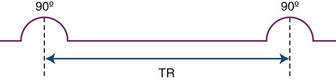
As mentioned before, the amount of the signal detected by the receiver coils depends on the magnitude of the net magnetization vector along the transverse or horizontal plane. Using certain operator-dependent parameters, it is possible to influence how much net magnetization strength (in other words, vector length) will be present in the transverse plane for the imaged tissues at the time of signal acquisition. During the imaging process, the initial 90-degree pulse flips the entire vertical or longitudinal magnetization vector into the horizontal plane. When this initial pulse is turned off, recovery along the longitudinal plane begins (T1 relaxation). Subsequent application of a second radiofrequency pulse at a given time after the first pulse will flip the net magnetization vector that recovered so far along the longitudinal plane back to the transverse plane. As a result, we can measure the magnitude of the net longitudinal magnetization that had recovered within each voxel at the time of application of the second pulse, provided that signal acquisition is begun immediately afterwards. The time between these radiofrequency pulses is referred to as repetition time, or TR (Fig. 33A.7). It is important to realize that contrary to the T1 and T2 times, which are properties of the given tissue, the repetition time is a controllable parameter. By selecting a longer TR, for instance, we allow more time for the net magnetization vector to recover before we flip it back to the transverse plane for measurement. A longer TR, because it increases the amount of signal that can potentially be detected, will also result in a higher signal-to-noise ratio, with higher image quality.
Tissue Contrast (T1, T2, and Proton Density Weighting)
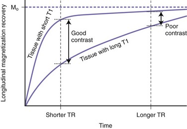
By using various TR and TE values, it is possible to increase (or decrease) the contrast between different tissues in an MR image. Achieving this contrast may be based on either the T1 or the T2 properties of the tissues in conjunction with their proton density. Selecting a long TR value reduces the T1 contrast between tissues (Fig. 33A.8). Thus, if we wait long enough before applying the second 90-degree pulse, we allow enough time for all tissues to recover most of their longitudinal or vertical magnetization. Because T1 is relatively short, even for tissues with the longest T1, this is possible without resulting in excessively long scan times. Since after a long TR, the longitudinally oriented net magnetization vectors of separate tissue types are all of similar magnitudes prior to being flipped into the transverse plane by the second pulse, a long TR will result in little T1 tissue contrast. Conversely, by selecting a short TR value, there will be significant variation in the extent to which tissues with different T1 relaxation times will have recovered their longitudinal magnetization prior to being flipped by the second 90-degree pulse (see Fig. 33A.8). Therefore, with a short TR, the second pulse will flip magnetization vectors of different magnitudes into the transverse plane for measurement, resulting in more T1 contrast between the tissues.
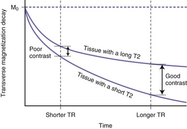
During T2 relaxation in the transverse plane, selecting a short TE will give higher measured signal intensities (as a short TE will not allow enough time for significant dephasing, i.e., transverse magnetization loss), but tissues with different T2 relaxation times will not show much contrast (Fig. 33A.9). This is because by selecting a short time until measurement (short TE) we do not allow significant T2-related magnitude differences to develop. If we select longer TE values, tissues with different T2 relaxation times will have time to lose different amounts of transverse magnetization, and therefore by the time of signal measurement, different signal intensities will be measured from these different tissues (see Fig. 33A.9). This is referred to as T2 contrast.
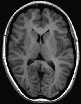
On T1-weighted images, substances with a longer T1 relaxation time (such as water) will be darker. This is because the short TR does not allow as much longitudinal magnetization to recover, so the vector flipped to the transverse plane by the second 90-degree pulse will be smaller with a lower resulting signal strength. Conversely, tissues with shorter T1 relaxation times (such as fat or some mucinous materials) will be brighter on T1-weighted images, as they recover more longitudinal magnetization prior to their proton spins being flipped into the transverse plane by the second 90-degree pulse (Fig. 33A.10). Among many other applications of T1-weighted images, they allow for evaluation of BBB breakdown: areas with abnormally permeable BBB show increased signal after the intravenous administration of gadolinium. Gadolinium administration is contraindicated in pregnancy. Breast-feeding immediately after receiving gadolinium is generally regarded to be safe (Chen et al., 2008). Renally impaired patients are susceptible to an uncommon but serious adverse reaction to gadolinium, nephrogenic systemic fibrosis (Marckmann et al., 2006).
On T2-weighted images, substances with longer T2 relaxation times (e.g., water) will be brighter because they will not have lost as much transverse magnetization magnitude by the time the signal is measured (Fig. 33A.11). The T1 and T2 signal characteristics of various tissues or substances found in neuroimaging are listed in Table 33A.1.
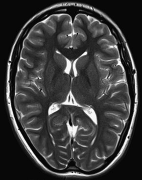
Table 33A.1 MRI Signal Intensity of Some Substances Found in Neuroimaging
| T1-Weighted Image | T2-Weighted Image | |
|---|---|---|
| Air | ↓ ↓ ↓ ↓ | ↓ ↓ ↓ ↓ |
| Free water/CSF | ↓ ↓ ↓ | ↑ ↑ ↑ |
| Fat | ↑ ↑ ↑ | ↑ |
| Cortical bone | ↓ ↓ ↓ | ↓ ↓ ↓ |
| Bone marrow (fat) | ↑ ↑ | ↑ |
| Edema | ↓ | ↑ ↑ |
| Calcification | ↓ (Heavy amounts of Ca++) ↑ (Little Ca++, some Fe+++) |
↓ |
| Mucinous material | ↑ | ↓ |
| Gray matter | Lower than in T2-WI | |
| White matter | Higher than in T2-WI | |
| Muscle | Similar to gray matter | Similar to gray matter |
| Blood products: | ||
| • Oxyhemoglobin | Similar to background | ↑ |
| • Deoxyhemoglobin | ↓ | ↓ |
| • Intracellular methemoglobin | ↑ ↑ | ↓ |
| • Extracellular methemoglobin | ↑ ↑ | ↑ ↑ |
| • Hemosiderin | ↓ | ↓ ↓ ↓ |
CSF, Cerebrospinal fluid; MRI, magnetic resonance imaging; T2-WI, T2-weighted image.
Magnetic Resonance Image Reconstruction
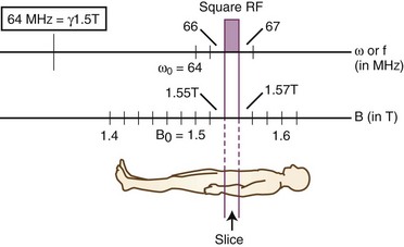
To construct an MR image, a slice of the imaged body part is selected, then the signal coming from each of the voxels making up the given slice is measured. Slice selection is achieved by setting the external magnetic field to vary linearly along one of the three principal axes perpendicular to the axial, sagittal, and coronal planes of the subject being imaged. As a result, protons within the slice to be imaged will precess at a Larmor frequency different from the Larmor frequency within all other imaging planes perpendicular to the axis along which the magnetic field gradient is applied. The Larmor frequency is the natural precession frequency of protons within a magnetic field of a given strength and is calculated simply as the product of the magnetic field, B0, and the gyromagnetic ratio, gamma. The precession frequency of a hydrogen proton is therefore directly proportional to the strength of the applied magnetic field. The gyromagnetic ratio for any given nucleus is a constant, with a value for hydrogen protons of 42.58 MHz/T. In slices at lower magnetic strengths of the gradient, the protons precess more slowly, whereas in slices at higher magnetic field strengths, the protons precess more quickly. Based on the property of nuclear magnetic resonance, the applied radiofrequency pulse (which flips the magnetization vector to the transverse plane) will stimulate only those protons with a precession frequency that matches the frequency of the applied radiofrequency pulse. By selecting the frequency of the stimulating radiofrequency pulse during the application of the slice selection gradient, we can choose which protons (those with a specific Larmor frequency) to stimulate (“make resonate”), and thereby we can select which slice of the body to image (Fig. 33A.12).
In the online version of this chapter (available at www.expertconsult.com), there is a discussion of the nature and application of the following MRI sequences or techniques: spin echo and fast (turbo) spin echo; gradient-recalled echo (GRE) sequences, partial flip angle; inversion recovery sequences (FLAIR, STIR); fat saturation; echoplanar imaging; diffusion-weighted magnetic resonance imaging (DWI); perfusion-weighted magnetic resonance imaging (PWI); susceptibility-weighted imaging (SWI); diffusion tensor imaging (DTI); and magnetization transfer contrast imaging.
Magnetic Resonance Imaging
Inversion Recovery Sequences (FLAIR, STIR)
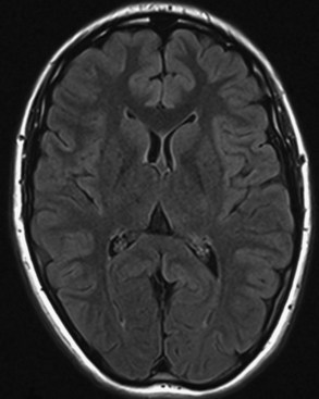
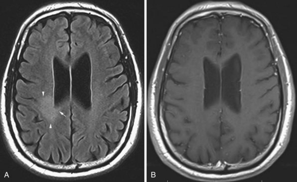
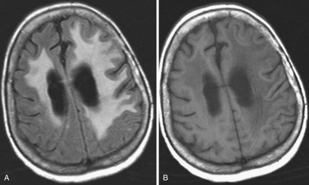
Inversion recovery techniques use a unique pulse sequence to avoid signal detection from the selected tissues (fat or CSF). Initially, a 180-degree radiofrequency pulse is applied. This will flip the longitudinal magnetization vectors of all tissues by 180-degrees, so that the vectors will point downward (south). Next, the flipped vectors are allowed to start recovering according to their respective T1 times. As the downward-pointing vectors recover, they become progressively smaller, eventually reaching zero magnitude, and from that point they start growing and pointing upward (north). Without interference, they recover the original longitudinal magnetization. However, during the process of recovery, after a time period referred to as inversion time (TI), a 90-degree pulse is applied. This will flip the longitudinal vectors to the transverse plane, where signal detection occurs. The amount of magnetization flipped by this pulse depends on how far the longitudinal recovery has been allowed to proceed. If the 90-degree pulse is applied when a given tissue’s vector happens to be zero (this is the so-called null point), no magnetization will be flipped from that tissue to the transverse plane, and therefore no signal will be detected from that tissue. Different tissues recover their longitudinal magnetization at different rates according to their specific T1 times. Knowing a given tissue’s T1 time, we can calculate when it will reach the null point (when its longitudinal magnetization is zero), and if we apply the 90-degree pulse at that point, we will not detect any signal from that particular tissue. The inversion time is linearly dependent upon a given tissue’s T1 value, being calculated as 0.69 multiplied by the T1 value. In the FLAIR (fluid-attenuated inversion recovery) sequence, the inversion time (when the 90-degree pulse is applied) occurs when the magnetization vector for the CSF is at the null point, so no signal will be detected from the CSF (Fig. 33A.13). In FLAIR images, the dark CSF is in sharp contrast with the hyperintensity of PV lesions, allowing their better identification. In STIR (short TI, or tau inversion, recovery) imaging, which is a fat-suppression technique, the methodology is essentially the same as for FLAIR. However, instead of CSF, the signal from fat is nulled. The TI for the STIR technique is set to 0.69 times the T1 of fat, which results in application of the final 90-degree pulse when the fat tissue’s magnetization is at the null point, so no signal from fat will be detected.
Fat Saturation
Fat saturation is a pulse sequence used to suppress the bright signal of adipose tissue and thereby allow better visualization of hyperintense abnormalities or, upon gadolinium administration, abnormal enhancement that otherwise may be obscured by fatty tissue in areas such as the orbits or spinal epidural space. In the same external magnetic field, the protons in fat versus water experience slightly different local magnetic fields because of differences in molecular structure. As a consequence, the protons in the fat will have a slightly different precession frequency from that of the water protons and will therefore resonate with a slightly different externally applied pulse frequency. Thus, it is possible to apply a radiofrequency pulse (presaturation pulse) that will resonate selectively with the fat-based protons only. This pulse will flip the magnetization vector of fat to the transverse plane, where it will be destroyed or “spoiled” by a gradient pulse. Next, the planned pulse sequence is applied, and at that point the obtained transverse magnetization will not have the component from fat, as it was destroyed (Fig. 33A.14). Therefore, by the time of TE, no signal will be detected from the fat tissue, and areas of fat will be dark in the image, allowing hyperintense enhancement to stand out.
Susceptibility-Weighted Imaging
SWI (Haacke et al., 2009; Mittal et al., 2009) uses a high spatial resolution 3D gradient echo imaging sequence. The contrast achieved by this sequence distinguishes the magnetic susceptibility difference between oxygenated and deoxygenated hemoglobin. Since the applied phase postprocessing sequence accentuates the paramagnetic properties of deoxyhemoglobin and blood degradation products such as intracellular methemoglobin and hemosiderin, this technique is very sensitive for intravascular venous deoxygenated blood as well as extravascular blood products. It has been used for evaluation of venous structures, hence the earlier name high-resolution blood oxygen level–dependent venography, but the clinical application is now much broader. Its exquisite sensitivity for blood degradation products makes this technique very useful when evaluating any lesion (e.g., stroke, AVM, cavernoma or neoplasm) for associated hemorrhage (Fig. 33A.15). It is also used for imaging microbleeds associated with traumatic brain injury, diffuse axonal injury, or cerebral amyloid angiopathy.
Diffusion Tensor Imaging
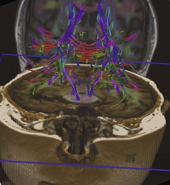
Diffusion tensor imaging is a more advanced type of diffusion imaging capable of quantifying anisotropy of diffusion in white matter. Diffusion is isotropic when it occurs with the same intensity in all directions. It is anisotropic when it occurs preferentially in one direction, as along the longitudinal axis of axons. For this reason, DTI finds its greatest current application in MRI examinations of the white matter. As opposed to characterizing diffusion within each voxel with just a single apparent diffusion coefficient, as in DWI, in DTI intravoxel diffusion is measured along three, six, or more gradient directions. The measured values and their directions are called eigenvectors. The vector that corresponds to the principal direction of diffusion (the direction in which diffusion is greatest in magnitude) is called the principal eigenvector. In normal white matter, diffusion anisotropy is high because diffusion is greatest parallel to the course of the nerve fiber tracts. Therefore, the principal eigenvector delineates the course of a given nerve fiber pathway. Diffusion tensor images can be displayed as maps of the principal eigenvectors which will show the direction/course of the given white matter tract (tractography). These images can also be color coded, allowing for more spectacular visualization of nerve fiber tracts (Fig. 33A.16). Any disruption of a given nerve fiber tract (e.g., MS, trauma, gliosis) will reduce anisotropy, and the disruption of the white matter tract can be visualized. Tensor imaging/tractography is useful in imaging of degenerating white matter tracts and also in surgical resection planning, when the anatomical relationship of the resectable lesion and the adjacent fiber tracts has to be evaluated to avoid or reduce surgical injury to critical pathways.
Magnetization Transfer Contrast Imaging
As the name indicates, magnetization transfer contrast imaging is a technique that produces increased contrast within an MR image, specifically on T1-weighted gadolinium-enhanced images and in magnetic resonance angiography (Henkelman et al., 2001). In water, hydrogen atoms are relatively loosely bound to oxygen atoms, and they move frequently between them, binding to one oxygen atom then switching to another. In other tissues (e.g., lipids, proteins), the hydrogen atoms are more tightly bound and tend to stay in one place for longer periods of time. Nevertheless, it does happen that a “bound” hydrogen in lipid or protein is exchanged with a “more free” hydrogen from water. In magnetization transfer imaging, at the beginning of the sequence a radiofrequency pulse is applied that saturates the bound protons in lipids and proteins but does not affect the free protons in water. In regions where magnetization transfer (i.e., exchange of saturated protons with free protons) occurs, the saturated protons will decrease the signal obtained from the imaged free protons. The more frequently this magnetization transfer occurs, the less signal is obtained from the region and the darker the region will be in the image. Magnetization transfer happens more frequently in the white matter, resulting in signal loss, and therefore on magnetization transfer images, the white matter appears darker. The CSF on the other hand, where magnetization transfer does not occur, does not lose signal. Magnetization transfer is minimal in blood because of the high amount of free water protons.
Structural Neuroimaging in the Clinical Practice of Neurology
Brain Diseases*
Brain Tumors
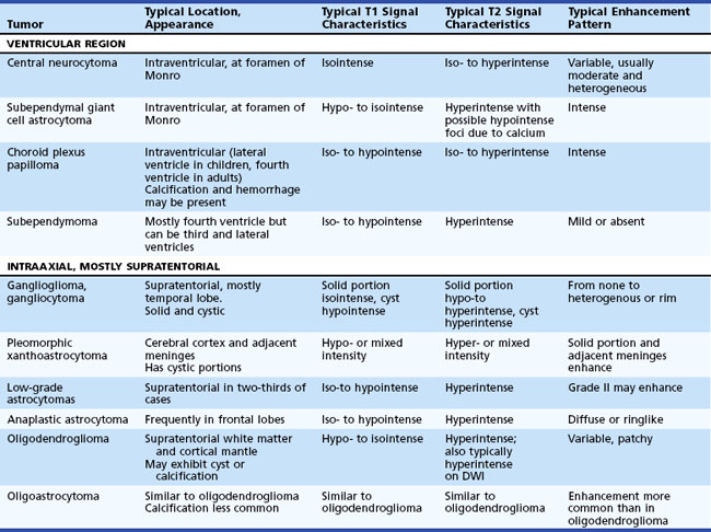
Epidemiology, pathology, etiology, and management of cancer in the nervous system are discussed in Chapter 52A, Chapter 52B, Chapter 52C, Chapter 52D, Chapter 52E, Chapter 52F, Chapter 52G . From the standpoint of structural neuroimaging, a useful anatomical classification distinguishes two main groups: intraaxial and extraaxial tumors. Intraaxial tumors are within the brain parenchyma, extraaxial tumors are outside the brain parenchyma (involving the meninges or, less commonly, the ventricular system). Intraaxial tumors are usually infiltrative with poorly defined margins. Conversely, extraaxial tumors, even though they often compress or displace the adjacent brain, are usually demarcated by a cerebrospinal (CSF) cleft or another tissue interface between tumor and brain parenchyma. For differential diagnostic purposes, intraaxial primary brain neoplasms can be further divided into the anatomical subgroups of supratentorial and infratentorial tumors (Table 33A.2).
Intraaxial Primary Brain Tumors
Ganglioglioma and Gangliocytoma
On MRI (Provenzale et al., 2000) the solid component is usually isointense on T1 and hypo- to hyperintense on T2-weighted images. The cystic component, if present, exhibits CSF signal characteristics. The associated mass effect is variable. With contrast, various enhancement patterns are seen—homogenous or rim pattern—but no enhancement is also possible.
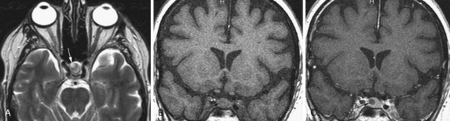
Pilocytic Astrocytomas
Pilocytic astrocytomas have two major groups: juvenile and adult. These tumors are classified as WHO grade I. Juvenile pilocytic astrocytomas are the most common posterior fossa tumors in children. The most common locations are the cerebellum, at the fourth ventricle, third ventricle, temporal lobe, optic chiasm, and hypothalamus (Koeller and Rushing, 2004). The appearance is often lobulated, and the lesion appears well demarcated on MRI. Hemorrhage and necrosis are uncommon. Areas of calcification may be present. The tumor usually exhibits solid as well as cystic components, with or without a mural nodule. The adult form is usually well circumscribed, often calcified, and typically exhibits a large cyst with a mural nodule. On MRI, the solid portions of the tumor are iso- to hypointense on T1 and iso- to hyperintense on T2-weighted images (Arai et al., 2006). The cystic component usually exhibits CSF signal characteristics. The associated edema and mass effect is usually mild, sometimes moderate. With gadolinium, the solid components (including the mural nodule) enhance intensely, but not the cyst, which rarely may show rim enhancement.
Pleomorphic Xanthoastrocytoma
Pleomorphic xanthoastrocytoma is a rare variant of astrocytic tumors. It is thought to arise from the subpial astrocytes and typically affects the cerebral cortex and adjacent meninges and may cause erosion of the skull. The most common location is the temporal lobe. It is classified as WHO grade II. It usually occurs in the second and third decades of life, and patients often present with seizures. On MRI (Tien et al., 1992) usually a well-circumscribed cystic mass appears in a superficial cortical location. A solid portion or mural nodule is often seen, and the differential diagnosis includes pilocytic astrocytoma and ganglioglioma. The signal characteristics are hypointense or mixed on T1, and hyperintense or mixed on T2-weighted images. With contrast, the solid portions and sometimes the adjacent meninges enhance. Calcification may be present. There is mild or no mass effect associated with this tumor.
Low-Grade Astrocytomas
Fibrillary astrocytomas, also termed diffuse astrocytomas, represent approximately 10% of all gliomas. Low-grade (WHO grade I and II) astrocytomas belong to this group (Figs. 33A.17 and 33A.18). These are well-differentiated tumors, usually arising from the fibrillary astrocytes of the white matter. Even though imaging may show a fairly well-defined boundary, these tumors are infiltrative and usually spread beyond their macroscopic border. Two-thirds of cases are supratentorial. A subgroup of these astrocytomas involves specific regions such as the optic nerves/tracts or the brainstem.
Oligodendroglioma
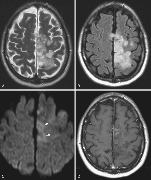
Oligodendroglioma accounts for 5% to 10% of all gliomas. It arises from the oligodendroglia that form the myelin sheath of the central nervous system (CNS) pathways. Oligodendroglioma occurs most commonly in young and middle-aged adults, with a median age of onset within the fourth to fifth decades and a male predominance of up to 2 : 1. Seizure is often the presenting symptom. The most common location is the supratentorial hemispheric white matter, and it also involves the cortical mantle. The tumor often has cystic components and at least microscopically, in 90% of cases also shows calcification. Hemorrhage and necrosis are rare, and the mass effect is not impressive. On MRI (Koeller and Rushing, 2005) the appearance is heterogenous, and the tumor is hypo- and isointense on T1 and hyperintense on T2. With gadolinium, the enhancement is variable, usually patchy, and the periphery of the lesion tends to enhance more intensely. Oligodendrogliomas are hypercellular and have been noted to appear hyperintense on diffusion-weighted images (Fig. 33A.19).
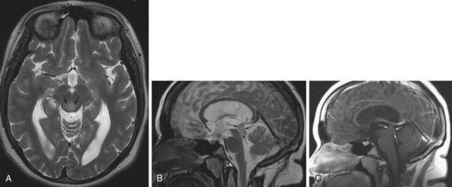
Gliomatosis Cerebri
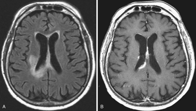
The MRI appearance is iso- to hypointense on T1 and hyperintense on T2. Hemorrhage is uncommon, and enhancement is also rare, at least in the early stages (Fig. 33A.20). Later, multiple foci of enhancement may appear, signaling more malignant transformation. The imaging appearance is similar to that of encephalitis, lymphoma, or subacute sclerosing panencephalitis, but in these disorders, clinical findings are more pronounced.
Glioblastoma Multiforme
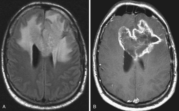
On MRI (Fig. 33A.21) glioblastomas usually exhibit mixed signal intensities on T1- and T2-weighted images. Cystic and necrotic areas are present, appearing as markedly decreased signal on T1-weighted and hyperintensity on T2-weighted images. Mixed hypo- and hyperintense signal changes due to hemorrhage are also seen. The hemorrhagic component can also be well demonstrated by gradient echo sequences or by SWI. The core of the lesion is surrounded by prominent edema, which appears hypointense on T1-weighted and hyperintense on T2-weighted images. Besides edema, the signal changes around the core of the tumor reflect the presence of infiltrating tumor cells and, in treated cases, postsurgical reactive gliosis and/or post-irradiation changes. Following administration of gadolinium, intense enhancement is noted, which is inhomogenous and often ringlike, also including multiple nodular areas of enhancement. The surrounding edema and ringlike enhancement at times makes it difficult to distinguish glioblastoma from cerebral abscess. DWI is helpful in these cases; glioblastomas are hypointense with this technique, whereas abscesses exhibit remarkable hyperintensity on diffusion-weighted images.
Lymphoma
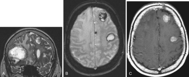
The imaging appearance of PCNSL depends on the patient’s immune status. The tumor is hypo- to isointense on T1-weighted and hypo- to slightly hyperintense on T2-weighted images. Contrast enhancement is usually intense. In immunocompetent patients (Zhang et al., 2010) the lesion is often single, tends to abut the ventricular border (Costa et al., 2006), and ring enhancement is uncommon (Fig. 33A.22). In immunocompromised patients, usually multiple, often ring-enhancing lesions are seen, which are most commonly located in the periventricular white matter and the gray/white junction of the lobes of the hemispheres, but the deep central gray matter structures and the posterior fossa may be involved as well. Overall, the imaging appearance appears more malignant in the immunocompromised cases and may be difficult to differentiate from toxoplasmosis. Other components of the differential diagnosis in patients with multiple PCNSL lesions include demyelination, abscesses, neurosarcoidosis, and metastatic disease.
Hemangioblastoma
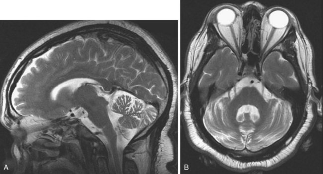
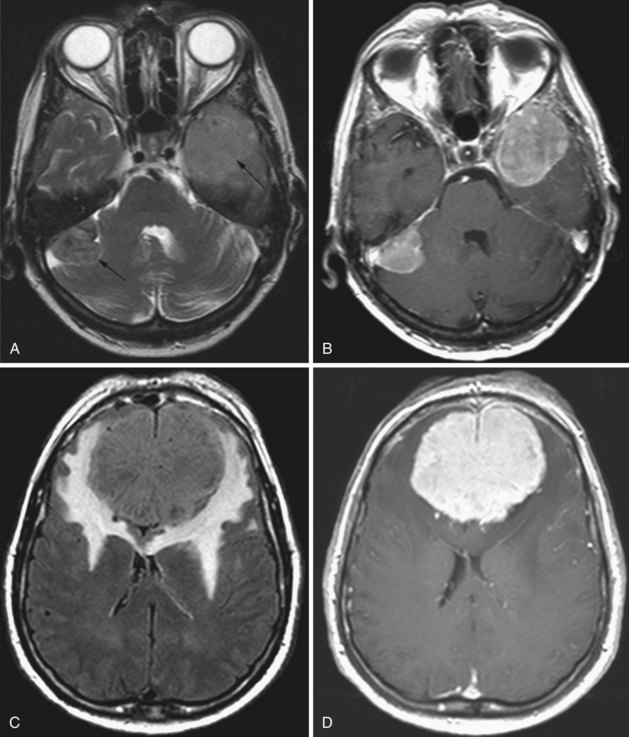
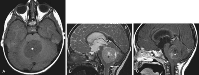
Hemangioblastomas represent only 1% to 2% of all primary brain tumors, but in adults they are the most common type of primary intraaxial tumor of the posterior fossa (cerebellum and medulla). These tumors are WHO grade I, well circumscribed, and exhibit a vascular nodule with a usually larger cystic cavity. On MRI the solid portion is hypo- to isointense on T1 and hyperintense on T2-weighted images. Sometimes hyperintense foci are noted on T1; this is due to occasional lipid deposition or hemorrhage within the tumor. The cystic component is usually hypointense on T1 (but may be hyperintense relative to CSF due to high protein content) and markedly hyperintense on T2. On FLAIR images, the cyst fluid is not completely nulled, resulting in bright signal, and the nodule is also hyperintense. There is usually mild surrounding edema. With gadolinium, the solid component exhibits intense enhancement. Hemangioblastomas are seen in 50% of patients with von Hippel-Lindau disease, and approximately one-fourth of all hemangioblastomas occur in these patients (Neumann et al., 1989).
Extraaxial Primary Brain Tumors
Descriptions of the rarer extraaxial primary brain tumor types—esthesioneuroblastoma, central neurocytoma, and subependymoma—are available in the online version of this chapter (www.expertconsult.com).
Meningiomas
Meningiomas are the most common primary brain tumors of non-glial origin and make up 15% of all intracranial tumors. The peak age of onset is the fifth decade, and there is a striking female predominance that may be related to the fact that some meningiomas contain estrogen and progesterone receptors. These tumors arise from meningothelial cells. In 1% to 9% of cases, multiple tumors are seen. The most common locations are the falx (25%), convexity (20%), sphenoid wing, petrous ridge (15% to 20%), olfactory groove (5% to 10%), parasellar region (5% to 10%), and the posterior fossa (10%). Rarely an intraventricular location has been reported. Meningiomas often appear as smooth hemispherical or lobular dural-based masses (Fig. 33A.23). Calcification is common, seen in at least 20% of these tumors. Meningiomas also often exhibit vascularity. The extraaxial location of the tumor is usually well appreciated owing to a visible CSF interface between tumor and adjacent brain parenchyma. Meningiomas may become malignant, invading the brain and eroding the skull. In such cases, prominent edema may be present in the brain parenchyma, to the extent that the extraaxial nature of the tumor is no longer obvious.
Schwannoma
Schwannomas arise from the Schwann cells of the nerve sheath, and the most commonly affected nerve is the vestibular portion of the vestibulocochlear nerve. They are typically bilateral in neurofibromatosis (NF) type 2 (see Fig. 33A.69). The unilateral form sporadically occurs in non-NF patients, with slight female predominance. Schwannomas typically arise in the intracanalicular segment of the eighth cranial nerve where myelin transitions from central (oligodendroglia) to peripheral (Schwann cell) type. If untreated, the tumor grows toward the internal auditory meatus and eventually bulges into the cerebellopontine angle, where it may deform and displace the brainstem. The intra- and extracanalicular parts of the tumor together result in a mushroom or ice cream cone–like appearance. The tumor is iso- to hypointense on T1-weighted images and iso- to hyperintense on T2-weighted images. This pattern may be modified by the presence of cystic changes or calcification. Gadolinium administration causes homogenous enhancement that, together with the performance of axial and coronal thin-slice T2-weighted images, allows for the visualization of even very small intracanalicular schwannomas.
Medulloblastoma
Medulloblastomas arise from the undifferentiated neuroectodermal cells of the roof of the fourth ventricle (superior or inferior medullary velum, vermis). They represent 25% of all cerebral tumors in children, usually presenting in the first and second decade. The tumor fills the fourth ventricle, extending rostrally toward the aqueduct and caudally to the cisterna magna, frequently resulting in obstructive hydrocephalus. Leptomeningeal and CSF spread may also occur, resulting in spinal drop metastases. Cystic components and necrosis may be present. Calcification is possible. On CT, medulloblastoma typically appears as a heterogeneous, generally hyperdense midline tumor occupying the fourth ventricle, with mass effect and variable contrast enhancement. The MRI signal (Koeller and Rushing, 2003) is heterogenous; the tumor is iso- or hypointense on T1 and hypo-, iso-, or hyperintense on T2. Contrast administration induces heterogenous enhancement (Fig. 33A.24). Restricted diffusion may be seen on DWI/ADC (Gauvain et al., 2001). Consistent with its site of origin, indistinct borders between the tumor and the roof of the fourth ventricle may be observed, aiding in the differential diagnosis, which in children includes atypical rhabdoid-teratoid tumor, brainstem glioma, pilocytic astrocytoma, choroid plexus papilloma, and ependymoma. The adult differential diagnosis includes the latter two entities in addition to metastasis and hemangioblastoma. Medulloblastoma does not tend to extrude via the foramina outside of the fourth ventricle, facilitating differentiation from ependymoma. In children, choroid plexus papilloma is more likely to occur within the lateral ventricle.
Extraaxial Primary Brain Tumors
Esthesioneuroblastoma
The cells of an esthesioneuroblastoma are derived from olfactory neuroepithelium neurosensory cells, hence its other name: olfactory neuroblastoma. This tumor characteristically extends through the cribriform plate to the anterior cranial fossa, orbit, and paranasal sinuses. Invasion of the brain is possible, and spreading via CSF has been described. The signal intensity of the tumor is variable. On MRI, T1-weighted signal is usually isointense relative to gray matter, while the T2-weighted signal varies from iso- to hyperintense (Schuster et al., 1994). With gadolinium administration, inhomogenous enhancement is seen.
Other Pineal Region Tumors
Pineocytoma
Pineocytomas are homogenous masses containing more solid components, but cysts may also be present. These tumors have a round, well-defined, noninvasive appearance. Calcification is commonly seen, but hemorrhage is uncommon. These tumors may be hypointense on T2 and exhibit a variable (central, nodular) pattern of intense enhancement after gadolinium administration (Fakhran and Escott, 2008).
Central Neurocytoma
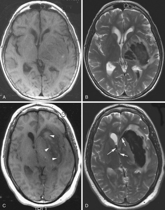
This neuron-derived tumor accounts for less than 1% of all primary brain tumors. It tends to appear in the fourth decade. The tumor is intraventricular, most commonly in the lateral ventricles anteriorly at the foramen of Monro, close to the septum and the columns of the fornix. Even though the tumor is relatively benign histologically, this location frequently leads to obstructive hydrocephalus. The MRI signal is heterogenous (Chang et al., 1993); the signal is isointense on T1 and iso- or hyperintense on T2 relative to the cortical gray matter. Calcification is possible, and cystic regions are also seen. Sometimes multiple cysts are noted, resulting in a “bubbly” appearance. The enhancement pattern is variable, but usually moderate and heterogenous.
Tumors in the Sellar and Parasellar Region
Pituitary Adenomas
The distinction between micro- and macroadenomas is based on their size: tumors less than 10 mm are microadenomas, the larger tumors are macroadenomas. These tumors may arise from hormone-producing cells, such as prolactinomas or growth hormone–producing adenomas, resulting in characteristic clinical syndromes. Pituitary adenomas are typically hypointense on T1-weighted and hyperintense on T2-weighted images, relative to the surrounding parenchyma. This signal change, however, is not always conspicuous, especially in the case of small microadenomas. Gadolinium administration helps in these cases, when the microadenoma is visualized as relative hypointensity against the background of the normally enhancing gland (Fig. 33A.25). Following a delay, this difference in enhancement is often no longer apparent, and if the postcontrast images are obtained in a later phase, a reversal of contrast may be noted. The adenoma takes up contrast in a delayed fashion and is seen as hyperintense against the more hypointense gland from where the contrast has washed out. Sometimes when the signal characteristics are not conspicuous, only alteration of the size and shape of the pituitary gland or shifting of the infundibulum may indicate the presence of a microadenoma. Because of this, it is important to be familiar with the normal range of pituitary gland sizes, which depend on age and gender. In adults, a gland height of more than 9 mm is worrisome. In the younger population, however, different normal values have been established. Before puberty, the normal height is 3 to 5 mm. At puberty in girls, the gland height may be 10 to 11 mm and may exhibit an upward convex morphology. In boys at puberty, the height is 6 to 8 mm, and the upward convex morphology can be normal. The size and shape of the gland may also change during pregnancy: convex morphology may appear, and a gland height of 10 mm is considered normal.
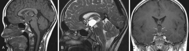
Craniopharyngioma
Craniopharyngiomas are believed to originate from the epithelial remnants of the Rathke pouch. This WHO grade I tumor may be encountered in children, and a second peak incidence is in the fifth decade (Eldevik et al., 1996). The most common location is the suprasellar cistern (Fig. 33A.26), but intrasellar tumors are also possible. The tumor may cause expansion of the sella or erosion of the dorsum sellae. In the suprasellar region, displacement of the chiasm, the anterior cerebral arteries, or even the hypothalamus is possible. Craniopharyngiomas have both solid and cystic components. Histologically, the more common adamantinomatous and the less common papillary forms are distinguished. The adamantinomatous type frequently exhibits calcification. The MRI signal is heterogeneous. Solid portions are iso- or hypointense on T1, whereas cystic components exhibit variable signal characteristics depending on the amount of protein or the presence of blood products. On T2, the solid and cystic components are sometimes hard to distinguish, as they are both usually hyperintense. Areas of calcification may appear hypointense on T2. With contrast, the solid portions of the tumor exhibit intense enhancement.
Metastatic Tumors
Intracranial metastases are detected in approximately 25% of patients who die of cancer. Cerebral metastases comprise over half of brain tumors (Vogelbaum and Suh, 2006) and are the most common type of brain tumor in adults (Klos and O’Neill, 2004). Most (80%) metastases involve the cerebral hemispheres, and 20% are seen in the posterior fossa. Pelvic and colon cancer have a tendency to involve the posterior fossa. Intracranial metastases, depending on the type of tumor, may involve the skull and the dura, the brain, and also the meninges in the form of meningeal carcinomatosis. Among all tumors that metastasize to the bone, breast and prostate cancer and multiple myeloma are especially prone to spread to the skull and dura. Most often, carcinomas involve the brain and get there by hematogenous spread. Systemic tumors with the greatest tendency to metastasize to brain are lung (as many as 30% of lung cancers give rise to brain metastases), breast (Fig. 33A.27), and melanoma (Fig. 33A.28). Cancers of the gastrointestinal tract (especially colon and rectum) and the kidney are the next most common sources. Other possibilities include gallbladder, liver, thyroid gland, pancreas, ovary, and testicles. Tumors of the prostate, esophagus, and skin (other than melanoma) hardly ever form brain parenchymal metastases.
Detection of intracerebral metastases is facilitated by administration of gadolinium, and every patient with neurological symptoms and a history of cancer needs to have a gadolinium-enhanced MRI study. The enhancement pattern of metastatic tumors can be solid or ringlike. To improve the diagnostic yield, triple-dose gadolinium or magnetization transfer techniques have been used, which improve detection of smaller metastases that are not so conspicuous with single-dose contrast administration. A triple dose of gadolinium improves metastasis detection by as much as 43% (van Dijk et al., 1997). Meningeal carcinomatosis can also be detected by contrast administration, which can reveal thickening of the meninges and/or meningeal deposits of the metastatic tumor.
Ischemic Stroke
Acute Ischemic Stroke
With the introduction of thrombolytic therapy in the treatment of acute ischemic stroke, timely diagnosis of an ischemic lesion, determining its location and extent, and demonstrating the amount of tissue at risk has become essential (see Chapter 51A). CT imaging remains of great value in the evaluation of acute stroke; it is readily available, and newer CT modalities including CT angiography and CT perfusion imaging are coming into greater use. The applicability of CT to acute stroke continues to be enhanced by the ever-increasing rapidity with which scans can be acquired, allowing for greater coverage of tissues with thinner slices. The technological advances allowing for rapid acquisition of data have led to 4D imaging, where complete 3D data sets of the brain are serially obtained over very short time intervals, allowing for higher temporal and spatial resolutions in brain perfusion studies of acute ischemic stroke patients.
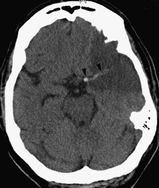
CT is very useful in detecting hyperdense hemorrhagic lesions as the cause of stroke. Early ischemic stroke, however, may not cause any change on unenhanced CT, making it difficult to determine the extent of the ischemic lesion and the amount of tissue at risk. CT is especially limited in evaluating ischemia in the posterior fossa, owing to streak artifacts at the skull base. Despite these limitations, early signs of acute ischemia on unenhanced CT may be helpful in the first few hours after stroke. CT signs of acute ischemia include blurring of the gray/white junction and effacement of the sulci due to ischemic swelling of the tissues. Blurring of the contours of the deep gray matter structures is of similar significance. In cases of internal carotid artery occlusion, middle cerebral artery main segment (M1) occlusion, or more distal occlusions, intraluminal clot may be seen as a focal hyperdensity, sometimes referred to as a hyperdense MCA, or hyperdense dot sign (Fig. 33A.29).
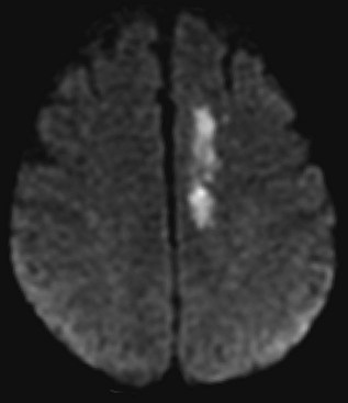
Several MRI modalities as well as CT perfusion studies are capable of providing data regarding cerebral ischemia and perfusion to assist in the evaluation for possible thrombolytic therapy very early after symptom onset. DWI with ADC mapping is considered to be the most sensitive method for imaging acute ischemia (Figs. 33A.30 to 33A.33 [Figs. 33A.31, B; 33A.32, B; and 33A.33 available online only]). In humans, the hyperintense signal indicating restriction of diffusion is detected within minutes after onset (Hossmann and Hoehn-Berlage, 1995).
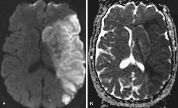
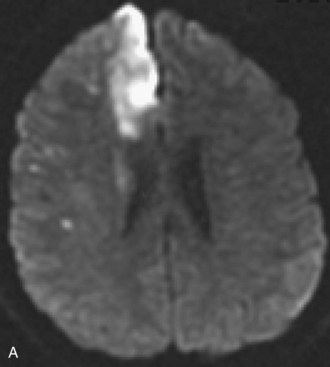
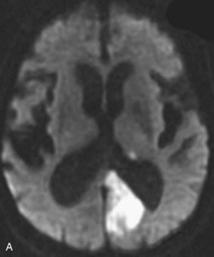
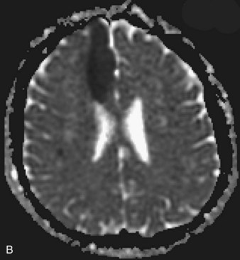
Fig. 33A.31 B, On apparent diffusion coefficient map, corresponding hypointensity is seen in the same area.
Temporal Evolution of Ischemic Stroke on Magnetic Resonance Imaging
Acute Stroke
Initially, the hyperintense signal on DWI is caused by decreased water diffusivity due to swelling of the ischemic nerve cells (for the first 5 to 7 days), then it increasingly results from the abnormal T2 properties of the infarcted tissue (T2 shine-through). For this reason, a reliable estimation of the age of the ischemic lesion is not possible by looking at DWI images alone. Imaging protocols for acute ischemic stroke usually include T1- and T2-weighted fast spin echo images, FLAIR sequences, and DWI with ADC maps. These sequences together confirm the diagnosis of ischemia, determine its extent, and allow for an approximate estimation of the time of onset (Srinivasan et al., 2006). On ADC maps, the values decrease initially after the onset of ischemia (i.e., the signal from the affected area becomes progressively more hypointense). This reaches a nadir at 3 to 5 days but remains significantly low until the seventh day after onset. After this time, the values increase (the signal gets more and more hyperintense) and return to the baseline values in 1 to 4 weeks (usually in 7 to 10 days). Therefore, ADC maps are quite useful for the estimation of the age of the lesion: if the signal of the area is hypointense on an ADC map, the lesion is likely less than 7 to 10 days old. If the area is isointense or hyperintense on the ADC map, the onset was likely more than 7 to 10 days ago. As already noted, although these signal changes take place on ADC maps, the DWI images remain hyperintense, without noticeable changes of intensity by visual inspection.
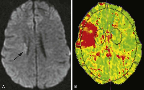
One purpose of MRI in the evaluation of acute stroke is to determine the extent of irreversible tissue damage and to identify tissue that is at risk but potentially salvageable. The combination of DWI and PWI is frequently used for this purpose (Fig. 33A.34). Evaluation is based on the premise that diffusion-weighted images delineate the tissue that suffered permanent damage (although in some cases, restricted diffusion is reversible, corresponding to ischemia without infarction), whereas areas without signal change on DWI but abnormal signal on perfusion-weighted images represent tissue at risk, the so-called ischemic penumbra. If there is a mismatch between the extent of DWI changes and perfusion deficits, the latter being larger, reperfusion treatment with intravenous or intraarterial thrombolysis or other intravascular techniques is justified to salvage the brain tissue at risk. If the extent of diffusion and perfusion abnormalities is similar or the same, the tissue is thought to be irreversibly injured, with no penumbra, and therefore the potential benefit from reperfusion treatment may not be high enough to justify the risk of hemorrhage associated with thrombolytic treatment.
Subacute Ischemic Stroke (1 Day to 1 Week after Onset)
Reperfusion usually occurs at this stage and may be associated with petechial hemorrhages or even frank hemorrhage within the infarcted tissue. Petechial hemorrhages are very common; microbleeds (not always visible with CT or MRI) occur in as much as 65% of ischemic stroke patients (Werring, 2007). Frank hemorrhagic transformation, however, is much less common.
Chronic Ischemic Stroke (3 Weeks and Older)
Areas of complete tissue destruction with death not only of neurons but of glia and necrosis of other supporting tissues as well, will eventually appear as cavitary lesions filled with fluid that have signal characteristics identical to CSF: hyperintensity on T2-weighted images and marked hypointensity on T1 images and FLAIR sequences. The region of encephalomalacia is bordered by a glial scar (reactive gliosis) that is hyperintense on T2 and FLAIR images (Fig. 33A.35; Fig. 33A.35, B available online only). Although the initial signal changes on DWI frequently predict the final extent of tissue destruction, changes on DWI can also disappear, and the final size of tissue cavitation can be best determined on T1-weighted images, which should be part of every stroke follow-up imaging protocol. Tissue in the margins of the cavitary lesion, and often in other areas of the brain as well, may have undergone extensive neuronal loss resulting only in atrophy but not in signal intensity changes, even on T2-weighted images (partial infarction).
Besides signal changes, chronic ischemic infarcts lead to secondary changes in the brain. Owing to the loss of tissue, ex vacuo enlargement of the adjacent CSF spaces (sulci and adjacent ventricular segments) occurs. Pathways that originate from or pass through the infarcted area undergo wallerian degeneration, which is seen as T2-hyperintense signal change along the course of these pathways (Fig. 33A.36). Later, the hyperintensity may resolve, but the loss of pathways may result in volume loss of the structures they pass through (e.g., cerebral peduncle, pons, medullary pyramid), noted as decreased cross-sectional area.
Stroke Etiology
Structural imaging provides data on the morphology and location of ischemic cerebral lesions, which can be very helpful to determine stroke etiology: lacunar, atherothrombotic, embolic, hypoperfusion-related, or venous. Diagnostic evaluation and treatment of a patient with stroke, as well as secondary stroke prevention, is often dependent upon structural imaging. A discussion of the neuroimaging aspects of the various stroke etiologies is in the online-only version of this book, available at www.expertconsult.com.
Stroke Etiology
Watershed Ischemic Stroke
These ischemic lesions involve the border zones between the vascular territories of the major cerebral arteries. Superficial border zone infarcts are between different major branches of the circle of Willis (such as anterior watershed infarcts between the anterior and middle cerebral arteries (see Fig. 33A.33) and posterior watershed infarcts between the middle and posterior cerebral arteries). Deep border zone infarcts develop between the superficial and deep branches of a cerebral artery.
Lacunar Ischemic Stroke
Lacunar ischemic strokes constitute 20% to 25% of all strokes and are typically seen in patients with hypertension and diabetes. This stroke type is thought to be due to narrowing and in situ thrombosis of the small, deep-penetrating arteries such as the lenticulostriate arteries. The most common locations include basal ganglia, internal capsule, and thalamus. According to structural imaging criteria, their size is usually less than 15 mm in diameter. Acutely, lacunar infarctions may exhibit restricted diffusion if the resolution of the ADC map is high enough to differentiate such from background signal variation. Chronic lacunes have a smoothly rounded, well-defined appearance. The encephalomalacic core of chronic lacunar infarctions follows CSF signal on all pulse sequences, appearing markedly hyperintense on T2 and hypointense on both T1 and FLAIR. There is often a thin rim of hyperintense signal on FLAIR due to gliosis, which helps differentiate lacunes from large Virchow-Robin spaces (Fig. 33A.37).
Other Cerebrovascular Occlusive Disease
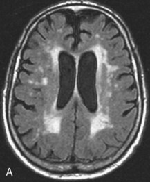
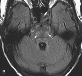
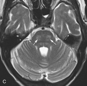
Microvascular Ischemic White Matter Lesions, “White Matter Disease,” Binswanger Disease
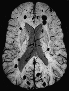
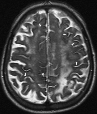
Chronic ischemic white matter lesions are hypodense on CT, but MRI is much more sensitive and reveals more extensive lesions (Fig. 33A.38; Fig. 33A.38, B-C available online only). On MRI, the lesions are hyperintense on T2 and FLAIR sequences. They may or not be visible as T1 hypointensities. It is possible that only lesions visible on T1-weighted images may be clinically significant. Common locations are the periventricular (PV) and more commonly, the deep white matter, but subcortical lesions are also common, with sparing of the U-fibers. The lesions can be isolated, scattered, or more confluent, especially in the PV zone. Morphologically, individual lesions generally exhibit indistinct borders with a diffuse “cotton-wool” appearance and range in size from punctate to small. Regions of confluent lesions may appear large and more commonly affect the deep white matter anterior and posterior to the bodies of the lateral ventricles, symmetrically within the parietal and frontal lobes. Deep white matter lesions also often occur in a distribution parallel to the bodies of the lateral ventricles on axial views, with an irregular band-like or “beads-on-string” appearance often separated from the PV lesions by an intervening band of relatively unaffected white matter. Involvement of the external capsules is also characteristic. These patterns of lesion distribution and morphology are often best seen on FLAIR. Contrary to the lesions of multiple sclerosis (MS), microvascular ischemia tends not to involve the temporal lobes or the corpus callosum. Besides the hemispheric white matter, microvascular ischemic lesions often also involve the basis pontis.
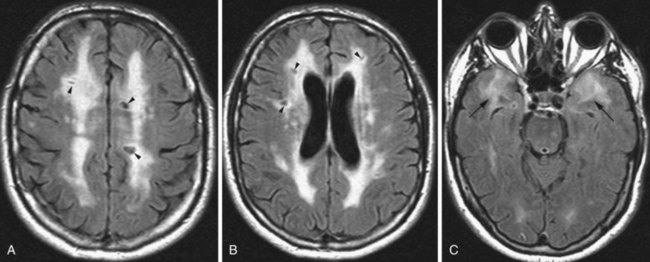
Cadasil
Cerebral autosomal dominant arteriopathy with subcortical infarcts and leukoencephalopathy (CADASIL) is an autosomal dominant inherited vascular disease. Pathologically there is destruction of the smooth muscle cells in the small and medium-sized penetrating arteries, with deposition of osmiophilic material and fibrosis leading to progressive thickening of the arterial wall and narrowing of the lumen. As a result, leukoencephalopathy and multiple ischemic strokes occur. Over 90% of patients have detectable mutations of the NOTCH3 gene, which encodes a transmembrane receptor primarily expressed in arterial smooth muscle cells. On MRI, multiple focal infarcts and T2-hyperintense white matter lesions are seen. The white matter lesions may involve the external capsules and, very characteristically, the anterior temporal lobe white matter in a confluent fashion that includes the subcortical arcuate fibers (Fig. 33A.39). This latter finding is helpful for the structural imaging diagnosis and helps distinguish CADASIL from “sporadic” ischemic arteriosclerotic vascular disease.
Cerebral Venous Sinus Thrombosis
Acute cerebral venous sinus thrombosis results in diminished or absent flow in the involved sinuses. Cerebral venous sinus thrombosis usually causes typical signal changes on MRI (Fig. 33A.40) and severely attenuated or absent flow signal on magnetic resonance venography (MRV). MRV techniques include flow-sensitive modalities such as 2D time of flight and phase contrast imaging, as well as postcontrast high-resolution 3D-SPGR, which offers excellent visualization of the sinuses with a very high spatial resolution and contrast-to-noise ratio.
Hemorrhagic Cerebrovascular Disease
Structural neuroimaging is crucial in the evaluation of hemorrhagic cerebrovascular disease. Besides detection of the hematoma itself, its location can provide useful information regarding its etiology. Lobar hematomas, especially along with small, scattered, parenchymal microbleeds, raise the possibility of cerebral amyloid angiopathy, whereas putaminal, thalamic, or cerebellar hemorrhages are more likely to be of hypertensive origin. Other underlying lesions such as brain tumors causing hemorrhages can be detected by structural imaging. This section discusses hemorrhagic cerebrovascular disease and cerebral intraparenchymal hematoma, whereas other causes of hemorrhage such as trauma or malignancy are discussed in other sections. Please also refer to Chapter 51B for a clinical neurological review of intracerebral hemorrhages.
Hyperacute Hemorrhage (0 to 24 Hours)
In the early (hyperacute) phase of intraparenchymal hemorrhage (<24 hours) the red blood cells are intact, and a mixture of oxy- and deoxyhemoglobin is present (Bakshi et al., 1998). In this stage, the signal on T1-weighted images is isointense to the brain, so even larger hematomas may be missed on this pulse sequence. On T2-weighted images, the oxyhemoglobin portion is hyperintense and deoxyhemoglobin is hypointense, resulting in the gradual appearance of a hypointense rim and gradually increasing hypointense foci within the hematoma as the amount of deoxyhemoglobin increases from the periphery. Such hypointense foci are also seen on FLAIR. Between the clot and the deoxyhemoglobin-containing rim, thin intervening clefts of fluid-like T2 hyperintensity may be seen as an initial manifestation of clot retraction. On gradient echo images, hyperacute hemorrhage will exhibit heterogeneously isointense to markedly hypointense signal, the latter corresponding to deoxyhemoglobin content in more peripheral portions of the clot. The amount of edema is mild in this stage, usually seen as a thin rim that is hyperintense on T2 and FLAIR images and hypointense on T1-weighted images (Atlas and Thulborn, 1998).
Acute Hemorrhage (1 to 3 Days)
During this stage, hemoglobin is transformed to deoxyhemoglobin, but the membranes of the erythrocytes are still intact (Bakshi et al., 1998). The hematoma becomes slightly hypointense on T1 and strikingly hypointense on T2-weighted images (Fig. 33A.41). On GRE, proton spins in the presence of paramagnetic deoxyhemoglobin dephase rapidly during TE, resulting in signal loss and, therefore, hypointensity of the hematoma on this pulse sequence. The surrounding edema, which is more extensive during this stage, is hypointense on T1 and hyperintense on T2.
Early Subacute Hemorrhage (3 Days to 1 Week)
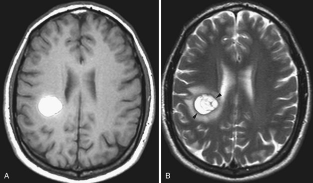
As blood degradation evolves, deoxyhemoglobin is converted to methemoglobin. At this stage, the blood degradation products are still intracellular (Bakshi et al., 1998). Intracellular methemoglobin is hyperintense on T1 and hypointense on T2-weighted images. T1 shortening is primarily the result of dipole-dipole interactions between heme iron and adjacent water protons, facilitated by a conformational change that occurs when deoxyhemoglobin is converted to methemoglobin.
Late Subacute Hemorrhage (1 to 4 Weeks)
In the late subacute phase, the membranes of the red blood cells disintegrate, and methemoglobin becomes extracellular (Bakshi et al., 1998). Extracellular methemoglobin contains Fe3+, which has five unpaired electrons. This leads to a dipole-dipole interaction which, contrary to intracellular methemoglobin, causes hyperintense signal change on both T1- and T2-weighted images (Fig. 33A.42).
Chronic Hemorrhage (>4 Weeks)
In the chronic stage (Bakshi et al., 1998), the core of larger hematomas turns into a slitlike or linear cavity with CSF signal characteristics, being hypointense on T1 and FLAIR and hyperintense on T2-weighted images. At the periphery of the lesion, macrophages continue to remove iron from the extracellular methemoglobin; hemosiderin and ferritin are deposited in their lysosomes, resulting in a rim of hypointense signal on T2-weighted and GRE images. This hypointense rim becomes progressively more prominent during the transition from the late subacute to chronic stage (Fig. 33A.43).
Superficial siderosis, a chronic sequela of bleeding into the subarachnoid space, and cerebral amyloid angiopathy, a hemorrhage-prone condition, are discussed in the online version of this book. Please visit www.expertconsult.com for more information.
Superficial Siderosis
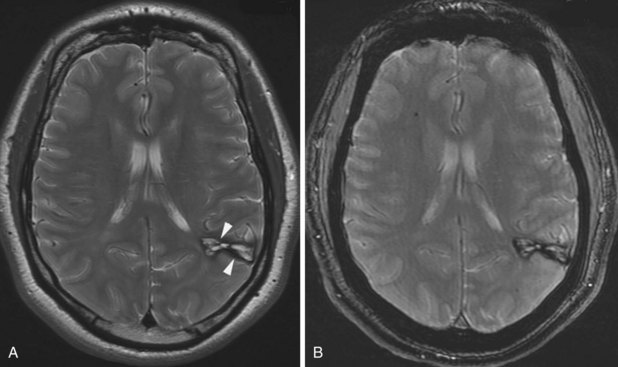
The phenomenon of superficial siderosis has been described as a late consequence of subarachnoid hemorrhage. It typically follows chronic or repeated episodic bleeding into the subarachnoid space. The recurrent hemorrhage can be due to certain tumors, trauma, or vascular malformations. As a result of the bleeding, there is deposition of hemosiderin into the subpial layer of the brain parenchyma. On T2-weighted images, this appears as a thin rim of hypointensity along the periphery of involved structures such as the cortical gyri, contour of the brainstem, rim of the spinal cord, or along certain cranial nerves (Fig. 33A.44). Although the phenomenon may be idiopathic, an extensive search for the earlier-described possible sources of hemorrhage is warranted.
Infection
Structural neuroimaging can provide useful information for evaluating infectious diseases of the CNS. The imaging modality of choice is MRI, which is able to demonstrate even subtle parenchymal abnormalities and inflammatory involvement of the meninges. For a review of the etiology, clinical presentation, and treatment of infections of the nervous system, see Chapter 53. And in addition to the neuroimaging features of infections discussed in the print version of this text, the online version includes features of CNS tuberculosis, cysticercosis, and cytomegalovirus. Please visit www.expertconsult.com for more information.
Cerebritis, Abscess
Cerebral abscesses are part of the differential diagnosis when ring-enhancing cerebral lesions are encountered. Besides the described ring morphology and the potential presence of daughter abscesses, cerebral abscesses exhibit restriction of diffusion centrally, appearing as hyperintense signal on diffusion-weighted images and hypointensity on ADC maps, which distinguishes them from metastatic and most primary brain tumors (Fig. 33A.45).
Infection
Herpes Simplex Encephalitis
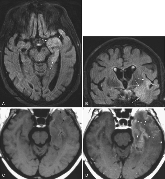
In adults, herpes encephalitis is caused by herpes simplex virus type 1. The imaging diagnosis is suggested by the location of the lesions. Herpes encephalitis typically involves the medial temporal and limbic frontal regions, including the basal frontal and cingulate gyri and insula. The cerebral cortex is more affected than the white matter. Herpes simplex encephalitis is usually hyperintense on T2 and FLAIR images and mildly hypointense on T1-weighted images (Fig. 33A.46). The encephalitis is frequently hemorrhagic, causing additional signal changes depending on the age of the hemorrhage. Areas of necrosis may be seen as well. Typically, a few days after onset, variable patterns of enhancement may be seen (gyriform, nodular, leptomeningeal, or intravascular). In the chronic stage, varying degrees of encephalomalacia, atrophy, calcification, and gliosis are seen in the affected lobes. Early successful treatment may minimize such sequelae.
Human Immunodeficiency Virus Encephalitis
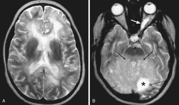
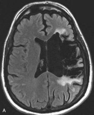
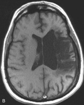
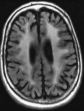
Human immunodeficiency virus (HIV) can affect the brain directly, causing a progressive encephalitis (formerly called AIDS dementia complex), or indirectly by making the host susceptible to opportunistic infections (cerebral toxoplasmosis, progressive multifocal leukoencephalopathy (PML), cytomegalovirus) and certain malignancies (lymphoma) that involve the CNS. HIV encephalitis microscopically appears as microglial nodules and multinucleated giant cells, with demyelination and vacuole formation. The demyelination is seen as hyperintense signal change on T2 and FLAIR images, usually starting in the PV white matter and centrum semiovale. Later the lesions become progressively more diffuse and confluent. Eventually, basal ganglionic and thalamic involvement is also seen. Along with these changes, prominent cerebral atrophy develops, with progressive enlargement of the central and superficial CSF spaces (Fig. 33A.47).
Cerebral Toxoplasmosis
In an HIV patient with cerebral lesions, the most common differential diagnostic consideration is lymphoma. The imaging appearance of HIV-related lymphoma is different from that seen in an immunocompetent host (see the brain tumor section of this chapter for details). Functional imaging with positron emission tomography (PET) or single-photon emission computed tomography (SPECT) may be used to differentiate between lymphoma and toxoplasmosis or other infectious lesions in HIV-positive patients (Heald et al., 1996).
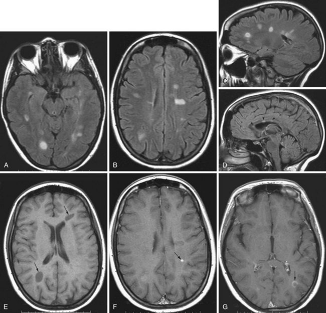
Progressive Multifocal Leukoencephalopathy
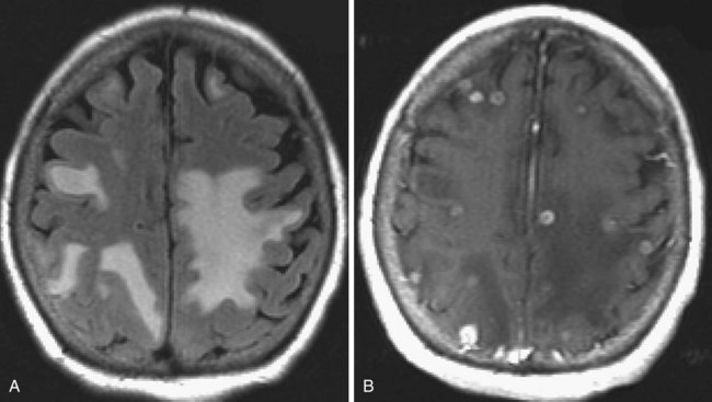
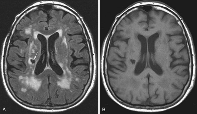
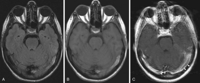
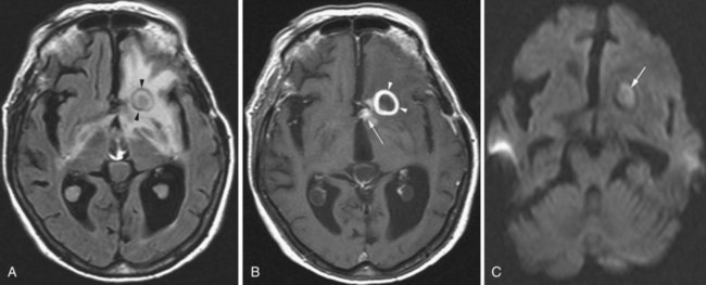
Progressive multifocal leukoencephalopathy is an infectious demyelinating disease caused by the JC polyomavirus. It has been most common in HIV patients, but it is now also a well-known potential complication of natalizumab infusions for MS. The disease initially involves the white matter, most commonly in the frontal, parietal, and occipital lobes. The lesions are hypointense on T1, hyperintense on T2 and FLAIR, usually multifocal, and are initially round or oval then become confluent. They tend to involve the subcortical white matter, including the U-fibers, with later involvement of the deep gray matter, corpus callosum, and posterior fossa. With gadolinium administration, faint enhancement may be present, but usually no enhancement is seen. DWI often reveals restricted diffusion at the spreading outer margins of PML lesions relative to the typically high ADC values within the gliotic and demyelinated central portions, which assists in the differential diagnosis (da Pozzo et al., 2006).
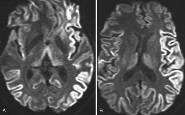
Creutzfeldt-Jakob Disease
Creutzfeldt-Jakob disease is a rapidly progressing, fatal dementing illness caused by prions—self-replicating, infectious protein particles. In advanced cases, MRI usually reveals prominent atrophy and gray-matter hyperintense signal changes on T2 and FLAIR sequences. The hyperintensity typically involves the cerebral cortex, basal ganglia, and cerebellum. There is no mass effect, and enhancement is rare. In the early stage of the disease, conventional T2-weighted images may be entirely normal, but diffusion-weighted images may show ribbonlike hyperintensity along the cerebral cortex (Fig. 33A.48), commonly involving the insula and cingulate cortex. Hyperintensity may be also seen in the caudate nucleus, lentiform nucleus, and in the thalamus as well, in a nonvascular distribution. Involvement of the pulvinar is characteristic of the mad-cow variant. Cerebellar cortical involvement is also common. The abnormalities may be uni- or bilateral. FLAIR sequences have been known to display these abnormalities earlier than conventional T2-weighted images, but not as conspicuously as DWI (Shiga et al., 2004; Young et al., 2005).
Multiple Sclerosis and Other Inflammatory or White Matter Diseases
Inflammatory and noninflammatory lesions of the corpus callosum, leukodystrophy (Krabbe disease, metachromatic leukodystrophy, adrenoleukodystrophy), radiation leukoencephalopathy, posterior reversible encephalopathy syndrome, and central pontine myelinolysis are discussed only in the online version of this chapter. Please visit www.expertconsult.com for more information.
Multiple Sclerosis
Multiple sclerosis is a demyelinating disease with autoimmune inflammatory reaction against the myelin sheath of CNS pathways (see Chapter 54). MRI is essential for the diagnosis of MS by demonstrating the typical inflammatory demyelinating lesions disseminated in time and space (Fig. 33A.49). It is also used for disease monitoring and assessment of response to therapy.
T1-weighted postcontrast images are useful for the detection of enhancing lesions in patients with clinical exacerbations. Enhancement may be solid or ringlike. Open-ring configurations are more typical for MS than other disease entities that also exhibit ring enhancement, such as tumors and infections (Masdeu et al., 2000). Five minutes between gadolinium injection and the acquisition of postcontrast images is the minimum acceptable delay for detecting acute demyelinating lesions, but longer delays of up to 30 minutes can significantly increase sensitivity, as can incorporation of magnetization transfer techniques and double or triple doses of gadolinium.
Chronic MS lesions do not exhibit restricted diffusion, appearing on DWI as either isointense to the surrounding brain parenchyma or, less commonly, hyperintense due to T2 shine-through artifact. On the corresponding ADC maps, chronic lesions exhibit normal or high apparent diffusion coefficients. However, as recently described, acute enhancing demyelinating lesions may on rare occasions exhibit high signal on DWI, with corresponding low pixel values (hypointense) on the ADC map, consistent with restricted diffusion (Balashov et al., 2009). Rapid resolution of restricted diffusion in these acute lesions is the rule, and they often evolve to exhibit increased ADC values on follow-up studies.
Inflammatory and Noninflammatory Lesions of the Corpus Callosum
In general neurological practice, the most commonly seen corpus callosum lesions are secondary to MS. FLAIR pulse sequences in the sagittal and axial planes are generally sufficient to assess corpus callosum pathology, although coronal views are also quite helpful. Isolated T2-hyperintense lesions within the central fibers of the genu, body, or splenium of the corpus callosum that are noncontiguous with the septocallosal margin are an uncommon finding. If such lesions exhibit a punctate or “snowball-like” appearance on sagittal views, Susac syndrome should be considered (see Chapter 15). Other small-vessel vasculitides can also result in small or punctate lesions within the corpus callosum.
An isolated medium-sized, bilaterally symmetrical lesion within the central fibers of the splenium that often also exhibits restricted diffusion is a transient finding in epilepsy (Polster et al., 2001) or metabolic encephalopathy (Takanashi et al., 2006). If patchy white-matter T2-hyperintensities are present in conjunction with a reversible splenial lesion, CNS lupus should be considered. When accompanied by multiple acute-appearing white and gray matter lesions, ADEM is more likely, and the corpus callosum lesion in this case is more likely to evolve to a chronic appearance. A T2-hyperintense lesion involving most of the central fibers of the splenium while sparing the periphery is typical of Marchiafava-Bignami disease; its typical morphology is best demonstrated on sagittal views.
The differential diagnosis (Uchino et al., 2006) for an isolated corpus callosum lesion also includes low-grade neoplasm if there is little to no mass effect and absent enhancement. If enhancement or mass effect is present, high-grade malignancies with a predilection for the corpus callosum (e.g., glioblastoma, primary CNS lymphoma), as well as metastases, are differential diagnostic considerations. Focal atrophy of the corpus callosum with overlapping T2-hyperintensity, contiguous with or near a region of cerebral hemispheric encephalomalacia and gliosis, is suggestive of wallerian degeneration. Diffuse axonal injury may also result in lesions of the corpus callosum and if suspected should be further evaluated with T2* or SWI to detect possible microhemorrhages.
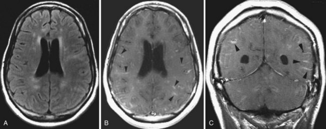
Neurosarcoidosis
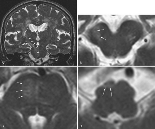
The prevalence of nervous system involvement in sarcoidosis is approximately 5%. In the brain parenchyma, multiple periventricular T2 hyperintense lesions are frequently noted, which may be due to a vasculitic process and often cannot be distinguished from MS or ischemic microvascular changes. Sarcoidosis may also involve the pituitary infundibulum and hypothalamus (resulting in endocrine symptoms). The granulomatous inflammation may affect the cranial nerves and/or their meningeal coverings as well, resulting in enlargement, hyperintense signal change, and abnormal enhancement. Although sarcoidosis may involve the dura, following gadolinium administration, leptomeningeal enhancement is more commonly noted. It is typically seen along the penetrating blood vessels and the adjacent leptomeninges, and is due to perivascular spread of the granulomatous process (Fig. 33A.50). Sometimes larger intraparenchymal or meningeal enhancing lesions are noted which may be mistaken for primary or metastatic tumors. When involved, the pituitary infundibulum and hypothalamus may also exhibit enhancement. Neurosarcoidosis may also lead to hydrocephalus, either by interfering with CSF absorption through the arachnoid granulations or by obstructing the ventricular system.
Leukodystrophy
Adrenoleukodystrophy
In adrenoleukodystrophy, there is abnormal metabolism of very long chain fatty acids. White matter changes, which are hypointense on T1 and hyperintense on T2 and FLAIR, typically start posteriorly and are seen in the parietal and occipital white matter around the atria of the lateral ventricles and across the splenium of the corpus callosum (Fig. 33A.51). T2-hyperintense signal change may be seen in the lateral geniculate bodies and along the corticospinal tracts. In the regions where active demyelination occurs, gadolinium enhancement may be seen. As the disease progresses, the white matter lesion distribution gradually involves more anterior regions.
Radiation Leukoencephalopathy
Radiation therapy may result in damage to the brain parenchyma, and this may happen at various time intervals after treatment (Bakshi et al., 1998). Acute radiation injury that happens during or a few days after treatment may not be seen on MRI. Sometimes, increased mass effect or more intense gadolinium enhancement may be seen in the irradiated area. In early delayed radiation damage, the changes appear in a few weeks or months after irradiation. Signal changes that are hypointense on T1 and hyperintense on T2 and FLAIR appear in the radiated region or in the PV white matter and basal ganglia in cases of whole brain radiation. These may enhance with gadolinium and tend to resolve in a few months. Late delayed radiation injury (which may be focal or diffuse) happens months or several years after treatment and usually follows longer treatment periods or higher radiation doses. The white matter changes (postirradiation leukoencephalopathy) start to appear in PV locations, and with time they become confluent around the borders of the ventricles. The changes can spread to other deep white-matter areas, seen confluently in the centrum semiovale (Fig. 33A.52). The involved white matter may exhibit areas of calcification. Ventricular and cortical sulcal enlargement is common. These changes are typically permanent.
Posterior Reversible Encephalopathy Syndrome
Posterior reversible encephalopathy syndrome (PRES) is thought to be due to abnormal cerebral vascular autoregulation resulting in vasogenic edema. A common etiology is severe hypertension (often in the setting of eclampsia or renal failure), but various medications can also cause it as a toxic side effect (tacrolimus, cyclosporin, FK-506, cyclophosphamide, interferons, and various chemotherapeutic agents). There is damage to the capillary endothelial junctions, vasodilatation resulting in fluid extravasation, and vasogenic edema. This condition has a predilection for the white matter of the posterior regions of the hemispheres, hence the former name of reversible posterior leukoencephalopathy syndrome (RPLS). In typical cases, variably extensive T1 hypointense and T2 hyperintense vasogenic edema is seen, usually symmetrically in the white matter of the parietal and occipital lobes (Fig. 33A.53). The name of the disease was changed after structural imaging revealed that gray matter, such as the basal ganglia and cerebral cortex, may also be involved (McKinney et al., 2007). It is also to be noted that at times the signal changes may be seen in the more anterior regions in the frontal and temporal lobes as well. With treatment of the underlying condition, such as hypertensive crisis or after withdrawal of the inciting agent, the clinical and imaging findings typically resolve.
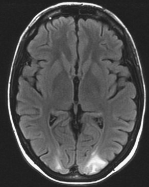
Central Pontine Myelinolysis
Central pontine myelinolysis has been described in cases of rapid correction of hyponatremia but also in malnutrition, alcoholism, and cases of hepatic insufficiency. MRI is the study of choice, and on T2-weighted images, striking hyperintense signal change is seen in the pontine tegmentum and basis pontis that characteristically spares the periphery and the corticospinal tract (Allen, 1984). At times, gadolinium enhancement may be seen at the periphery of the lesion, but usually no enhancement is seen. Although the typical location is the pons, regions of extrapontine demyelination can also be seen in a minority of patients, including the basal ganglia, thalamus, cerebellum, and within the hemispheres.
Trauma
Both CT and MRI have a pivotal role in the evaluation of craniocerebral trauma (Chapter 50B). In the emergency room setting, the first imaging modality is usually a noncontrast CT scan. CT bone windowing is the best tool for evaluating skull fractures (Fig. 33A.54), whereas brain windowing is of great value for visualizing subarachnoid, epidural, subdural, intraventricular, or intraparenchymal hemorrhages. MRI is very useful in detecting traumatic lesions of the brain parenchyma, especially when more subtle changes are present, such as small contusions, parenchymal microbleeds, and the small or punctate lesions of diffuse axonal injury. The various consequences of trauma that we will review next seldom occur in isolation but tend to occur in various combinations (e.g., cortical contusion is frequently associated with subarachnoid hemorrhage).
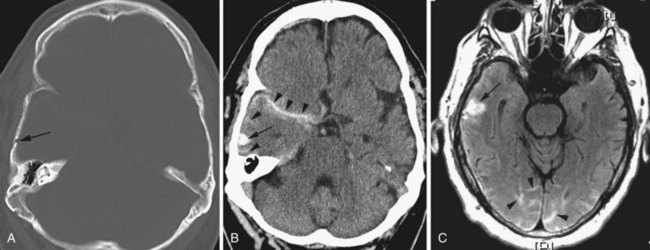
Traumatic Subarachnoid Hemorrhage
Until FLAIR pulse sequences became available, MRI was inferior to CT in detecting subarachnoid blood, especially in the first few days. Conventional T1- and T2-weighted images may completely miss subarachnoid blood in these early stages. However, subarachnoid blood appears hyperintense on FLAIR images (see Fig. 33A.54), and this pulse sequence is considered equal or superior to CT in detecting subarachnoid blood (Woodcock et al., 2001), especially in the posterior fossa and at the skull base, where CT images are often compromised by beam-hardening artifacts. The hyperintense signal change is due to the presence of blood, which changes the zero point of the inversion time of CSF, and therefore signal attenuation in subarachnoid regions containing hemorrhage will not be complete. An important caveat is that subarachnoid hyperintensity on FLAIR may also result from other causes. A common cause is magnetic susceptibility artifact, seen in patients who have braces or other metal devices that distort the magnetic field, which results in a lack of CSF signal suppression and the artifactually hyperintense appearance of CSF adjacent to the anterior frontal lobes.
Besides detection of blood in the acute phase, structural neuroimaging is also very useful to evaluate the potential later complications of subarachnoid hemorrhage. Subarachnoid blood may occlude the arachnoid granulations, leading to impaired CSF absorption, communicating hydrocephalus, and ventriculomegaly. Another late phenomenon that tends to follow repeated episodes of subarachnoid hemorrhage is superficial siderosis. In this condition, hemosiderin is deposited along the leptomeninges and appears as linear areas of hypointensity on T2-weighted images (see Fig. 33A.44 online at www.expertconsult.com).
Subdural Hemorrhage
On MRI, subdural hematomas exhibit a signal evolution similar to that seen with intraparenchymal hemorrhages, but the pace of evolution is different due to a slower decrease of the oxygen content within the hematoma. Acute subdural hematomas (Fig. 33A.55) are initially isointense on T1 and hyperintense on T2, but as deoxyhemoglobin appears, the signal on T2-weighted images becomes hypointense. In the subacute phase, the signal is hyperintense on T1 and hypointense on T2, but in the late subacute stage, the signal will be hyperintense on both T1- and T2-weighted images because of extracellular methemoglobin (Fig. 33A.56). It is important to remember that these stages are not separated sharply, and mixed patterns are often seen; this is due to the presence of oxy- and deoxyhemoglobin in the acute stage and intra- and extracellular methemoglobin in the chronic stage. Rebleeding into an existing subdural hematoma may also occur, resulting in the presence of clots of various ages.
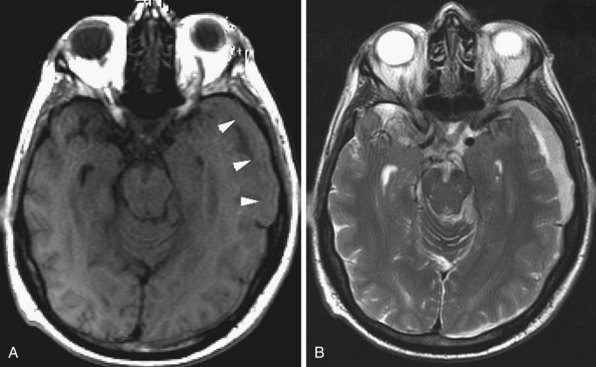
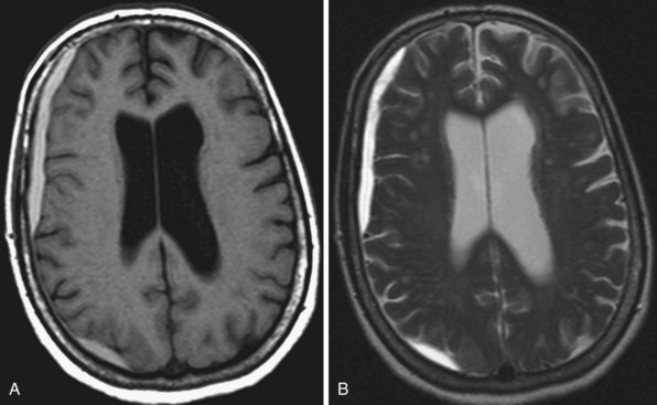
Chronic subdural hematomas (Fig. 33A.57) are hypointense relative to the brain but, having higher protein content, are mildly hyperintense relative to the CSF on T1-weighted images and hyperintense on T2-weighted images. Hemosiderin deposition is not as prominent as in parenchymal hemorrhages because macrophages tend to be cleared by the meningeal circulation. Chronic subdural hematomas may look similar to hyperacute ones on noncontrast images, but because of their vascular membrane, with gadolinium they exhibit enhancement along their periphery. On CT, chronic subdural hematomas appear as hypodense subdural collections. Mass effect is variable depending on the size of the hematoma and degree of cerebral atrophy. If repeated hemorrhage occurs into the subdural collection, the hyperdense fresh blood is seen within the chronic hypodense collection (Fig. 33A.58).
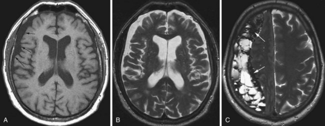
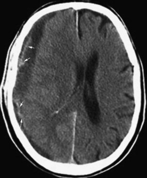
Cortical Contusion
Cerebral contusions result from the brain hitting against the inner table of the skull or sliding against the bony ridges of the base of the skull. The most common locations include the poles and inferior surfaces of the frontal, temporal, and occipital lobes. The injured brain parenchyma exhibits foci of hemorrhage and varying degrees of edema, which may progress later to more confluent hematoma and more swelling. On CT, acute contusions appear as foci of hyperdense hemorrhage with or without swelling. The hematomas get reabsorbed later, and the swelling decreases. In the chronic stage, no residual findings or varying degrees of encephalomalacia may be seen. On MRI, with the appearance of deoxyhemoglobin, a hypointense signal is seen on T2; the surrounding edema is hyperintense on T2 and FLAIR sequences (Fig. 33A.59). Later, in the subacute stage, extracellular methemoglobin is hyperintense on T1- and T2-weighted images. Gradient echo and susceptibility-weighted images are very useful to show the hemorrhagic component of the lesion. Chronic contusions are associated with encephalomalacic cavities of various sizes, exhibiting CSF signal characteristics and surrounded by a hyperintense rim of reactive gliosis on T2 and FLAIR sequences. Variable degrees of hemosiderin deposition appear hypointense on FLAIR, gradient echo, and SWI.
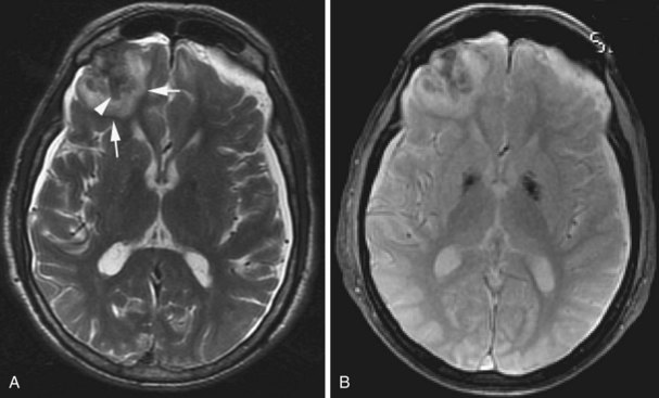
Diffuse Axonal Injury
The underlying pathomechanism of this entity is shearing injury of the white matter pathways. This may involve the corpus callosum, other fiber tracts of the corona radiata and centrum semiovale, and may also involve the brainstem. The changes on structural neuroimaging can be very subtle, usually in the few-millimeter size range. Such lesions are usually not detected by CT. MRI is the study of choice. On MRI, the lesions appear as foci of hyperintensity seen on T2 and FLAIR sequences. Foci of hemorrhage (usually microbleeds) are also present. For detection of the microbleeds associated with axonal injury, gradient echo or susceptibility-weighted images (Fig. 33A.60) are the most sensitive (Li and Feng, 2009).
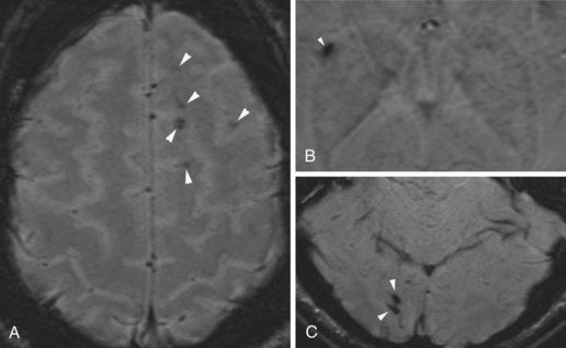
Metabolic and Toxic Disorders
This section is in the online-only version of this chapter. Please visit www.expertconsult.com for more information, and also refer to Chapters 56 through 58 and 62 for further discussions of these topics.
Metabolic and Toxic Disorders
Mitochondrial Disease
Mitochondrial diseases (Chapter 63) cause cellular metabolic disturbances. Most often responsible are mutations in mitochondrial DNA or in nuclear genes that regulate mitochondrial function. Tissues with high metabolic activity such as brain and skeletal muscle are preferentially affected. Various syndromes belong to this group of metabolic disorders, the most common being MELAS (mitochondrial encephalomyopathy with lactic acidosis and stroke-like episodes), Kearns-Sayre syndrome, MERRF (myoclonic epilepsy with ragged-red fibers), and Leigh disease.
Genetic and Degenerative Disorders Primarily Causing Ataxia (Cerebellar Disorders)
Structural neuroimaging has a limited role in the evaluation of hereditary and degenerative cerebellar disorders. The neurological examination, family history, and genetic testing are most helpful in finding the specific diagnosis, whereas imaging usually has a supportive role—for instance, by defining the degree of involvement of the pontine nuclei in the differential diagnosis of olivopontocerebellar atrophy. Nevertheless, imaging is almost always obtained in patients who present with progressive ataxia for the purpose of ruling out other potential causes, such as an enlarging posterior fossa neoplasm. Additionally, certain ataxic disorders (multiple system atrophy, spinocerebellar ataxias, Friedrich ataxia, ataxia-telangiectasia, fragile X premutation syndrome) may present with characteristic MRI changes. These are discussed in the online-only version of this chapter (visit www.expertconsult.com). Please also refer to Chapters 20 and 72 for review of ataxic disorders.
Genetic and Degenerative Disorders Primarily Causing Ataxia (Cerebellar Disorders)
Multiple System Atrophy, Cerebellar Subtype
In the cerebellar subtype of MSA, predominantly infratentorial structures are affected, hence the other name for this entity, olivo-ponto-cerebellar atrophy (OPCA). There may be atrophy of the olivary eminences of the medulla, which is well appreciated on thin-slice axial images. In the pons, a horizontal T2 hyperintense signal change may be noted, characteristically involving the transverse pontine fibers, and often a vertical linear hyperintensity is also seen, corresponding to the degenerating neurons of the raphe nuclei. The constellation of these linear T2 hyperintense areas that cross each other perpendicularly is referred to as the hot-cross-bun sign. Although this sign has been thought to be specific for MSA-c, it has also been described in the other two MSA subtypes, spinocerebellar ataxia (types 2 and 3), parkinsonism with vasculitis (Muqit et al., 2001), fragile X premutation tremor/ataxia syndrome, and in variant Creutzfeldt-Jakob disease (Soares-Fernandes et al., 2009). Another potential finding in MSA-c is T2 hyperintense signal change, extending into the middle cerebellar peduncles in a symmetrical fashion. This finding is not pathognomonic—for instance, occurring also in fragile X premutation tremor ataxia syndrome.
Spinocerebellar Ataxias
Spinocerebellar ataxias (SCA, types 1-29) are genetically heterogeneous disorders resulting in expansion of glutamine-coding CAG triplets of the involved genes. The resultant abnormal proteins (containing polyglutamine) are felt to have a pathogenetic role. In these diseases, variable degrees of cerebellar, brainstem, and spinal cord atrophy are seen with imaging (Fig. 33A.61). The structural imaging appearance is not specific but supports the diagnosis. SCA type 6 is a pure cerebellar syndrome that stands out from the structural imaging standpoint in that there is little extracerebellar atrophy, and the atrophy predominantly involves the vermis, especially the superior vermis. This imaging appearance is similar to that seen in chronic alcohol abuse or phenytoin-related cerebellar toxicity, which are the main differential diagnostic considerations.