Ventricular Function: Cine Imaging

For the assessment of ventricular function (e.g., assessment of left ventricular wall motion), images of the heart at multiple time points or phases in the cardiac cycle are acquired. An optimal MRI pulse sequence provides good contrast between the ventricular blood pool and the myocardium, and high spatial and high temporal resolution. Gradient-recalled-echo (GRE) techniques are typically used. A variant of steady-state GRE acquisition, balanced steady-state free precession (SSFP), has gained acceptance as the primary method for cardiac cine imaging at 1.5 T. Gradient-echo imaging is still used at 3.0 T, however, because of the sensitivity of balanced SSFP to off-resonance effects that can cause significant black banding and ghosting image artifacts. The balanced SSFP pulse sequence (depending on MRI scanner manufacturers known as trueFISP, FIESTA, or balanced-FFE) yields the highest image SNR by refocusing all available magnetization at the end of each sequence repetition period (TR).^8,9

Images acquired at different cardiac time points are played back in a movie loop to enable the assessment of the contractile function of the left ventricle—hence the name cine (referring to the motion picture technique). There are several techniques for generating a cine series. Because the imaging pulse sequence is unable to complete image acquisition within the 25- to 100-ms time frame of a phase in the cardiac cycle, the acquisition is segmented over several cardiac cycles. As shown in Figure 13-1A, the number of views, or k-space lines, acquired in a cardiac cycle, or R–R interval, is known as the views-per-segment (vps). Segments are acquired repeatedly throughout the cardiac cycle, with each segment at a different temporal phase, starting from the R wave trigger. This segment acquisition continues until the next cardiac R wave trigger is encountered, at which time the next set of k-space encoding views are updated, and the process is repeated until all k-space encoding views have been acquired. An acquisition that is prescribed for a phase encoding matrix dimension of 128 requires a total of 128 views and 16 heartbeats to complete, using 8 vps (128 views ÷ 8 vps = 16 segments; 1 segment per heartbeat for a total of 16 heart beats).

FIGURE 13-1 A, In a segmented k-space acquisition, k-space encoding lines are acquired continuously throughout the cardiac cycle. In this example, with 4 vps, only n = 9 segments can fit into the R–R interval (segments labeled 1, 3, 5, … , 17). B, To double the number of phases using view sharing effectively, the nearest k-space lines from adjacent segments are combined (shared) to form an intermediate segment that lies midway in time between the acquired segments (2, 4, 6, … , 16). These new interpolated segments together with the acquired segments now yield (2n − 1) reconstructed cardiac phases.

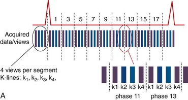
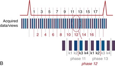
All of the data from each segment, when reconstructed, characterize the heart at the corresponding time or cardiac phase within the R–R interval. For segmented acquisitions, it is assumed that the heart is in the same cardiac phase for the same cardiac delay time as measured from the R–R interval, for all cardiac cycles. The acquired temporal resolution (Δt) of the cine sequence is simply:

(1)

where TR is repetition time. The number of acquired cardiac phases that can fit into an R–R interval is limited by the temporal resolution of the acquisition and the patient’s heart rate. The number of acquired phases is:

(2)

where avail_RRtime is the cardiac R–R interval time and is given (in ms) as:

(3)

where the heart rate is given in beats per min and trig_window is the fraction of the cardiac R–R interval where data acquisition is disabled to wait for the next cardiac R wave trigger. The number of heart beats that are required to reconstruct an image is given by:

(4)

where yres is the image resolution in the phase-encoding direction and represents the number of k-space lines in the image.

For a heart rate of 80 beats/min, TR = 5 ms, and vps = 12, with a 10% trigger window (trig_window = 0.10), 11 phases or segments can be acquired per cardiac interval. For fast heart rates and low temporal resolution, the number of acquired phases is small, and does not allow a smooth depiction of cardiac motion. The effective temporal resolution can be substantially increased, however, using view sharing.¹⁰

View sharing effectively doubles the number of reconstructed cardiac phases by sharing k-space lines between adjacent acquired data segments to generate an intermediate-phase image. As shown in Figure 13-1B, where a view-sharing factor of 2 is used for a 4-vps acquisition, k-space encoding lines k1, … , k4 are acquired in each segment. To generate an intermediate phase image, k-space encoding lines k3 and k4 from segment n are combined with k-space encoding lines k1 and k2 lines from segment n + 1 to form an intermediate time point or phase image between acquired phases n and n + 1.

This nearest neighbor interpolation reconstructs an image at a time point midway between two adjacent acquired phases. Although the acquired temporal resolution is still given by Equation 1, the effective temporal resolution is now doubled to:

(5)

where vvs is the view sharing factor, and typically, vvs = 2.

One disadvantage of view sharing or nearest neighbor interpolation is that not all of the cardiac R–R interval is fully imaged. Because of the trigger window at the end of the cardiac interval, visualization of end-diastolic function, such as end-diastolic atrial contraction, is impossible with prospective gating techniques. Another disadvantage of prospective gating with view sharing is that the number of reconstructed phases (2n_phases − 1) varies according to the heart rate. This variation makes functional assessment of wall motion at different slice locations quite difficult, if the number of phases in each location is different because of changes in the patient’s heart rate during the cardiac cine examination.

With the increased speed in computational hardware, imaging of the complete cardiac cycle is now possible, eliminating the dead time at the end of the cardiac R–R interval. This improvement comes with the ability of MRI systems to monitor events in real time and effect a change in the pulse sequence in response. For full R–R coverage, the cardiac R wave trigger event is monitored in each TR interval. If a valid cardiac trigger is detected, the k-space encoding views are updated, and data acquisition continues until all k-space views are collected.

The number of acquired segments for each cardiac R–R interval can change owing to possible variations in the patient’s heart rate. These variations in the number of segments and the R–R interval are tracked over time, however, by the MRI scanner’s computer or real-time data processor. After data acquisition is complete for each cardiac cycle, the acquired views for each cardiac R–R interval are sorted retrospectively and binned or interpolated into the appropriate cardiac phase.¹¹ As shown in Figure 13-2, with retrospective gating or sorting, we can choose to reconstruct an arbitrary number of phases for any given number of actual acquired segments. With retrospective interpolation, each cardiac R–R interval is divided into equal time points. The acquired views for each cycle are interpolated to each reconstructed time point using a linear interpolation scheme.

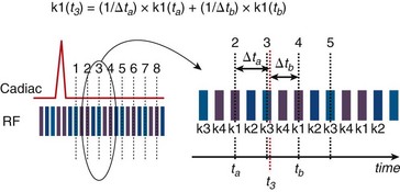
FIGURE 13-2 Diagram illustrating the retrospective reconstruction of cine cardiac phases. In this example with 4 vps, the R–R interval is divided into equal intervals. For the third cardiac phase (t = t₃), the closest k1 encoded lines occur at times t = t_a and t = t_b. To calculate the k1 encoded line at time t = t₃, a linear interpolation is performed between the closest k1 acquired views with an inverse weighting of the time from t = t₃ (shown as Δt_a and Δt_b).

Because the cardiac phase is defined as the fraction (in time) of the cardiac R–R interval, k-space views from different cardiac cycles interpolated to the same cardiac phase regardless of the actual delay time of that time point from the R wave trigger are good representations of the cardiac motion at that phase of the cardiac cycle. The same, fixed number of phases can be acquired for every patient, yielding cine data sets with a standard number of reconstructed cardiac phases, independent of the patient’s heart rate. By using this retrospective approach, events over the full cardiac cycle can be easily captured.

Black Blood Imaging

To visualize the cardiac anatomy, black blood imaging, typically a T2-weighted spin-echo pulse sequence, is often used. Because blood returns high signal intensity with T2-weighted pulse sequences, blood suppression techniques are applied to prevent the bright blood signal from masking abnormal structures in the myocardium. As with cine acquisitions, a segmented k-space approach is also used for T2-weighted cardiac imaging. In a segmented k-space FSE acquisition, the primary spin-echo formed after the RF excitation pulse is repeatedly refocused by a series of 180-degree RF pulses and forms a train of spin-echoes. Each spin-echo in the train is encoded for a different k-space view. Multiple k-space views are encoded for a single RF excitation pulse. The number of echoes (echo train length [ETL]) acquired per RF excitation pulse is analogous to the vps in cine scans. Strong T2-weighting can be achieved at a fraction of the time required to acquire a conventional spin-echo image. With an ETL = 16, a gated FSE image can be acquired in 8 to 16 heartbeats, depending on the desired in-plane spatial resolution.

Blood suppression is achieved by using a double inversion recovery (IR) technique.¹² As shown in Figure 13-3, a nonselective IR RF pulse inverts all spins in the RF coil volume. This inversion is followed immediately by a slice-selective IR RF pulse to restore the longitudinal magnetization only within the imaged slice. The aim of the reinversion RF pulse is to ensure that the spins within the imaged slice are unperturbed. At an appropriate inversion time (TI), selected so that TI = TI_null,blood, the point in time where the inverted longitudinal magnetization of blood is zero (TI_null,blood = T_1,blood log_e 2), the FSE image acquisition is applied. In this TI interval, blood within the imaged slice is replaced with blood from outside the slice (with inverted longitudinal magnetization). At the moment of data acquisition (just after application of the 90-degree RF excitation pulse), the longitudinal magnetization of blood passes through zero resulting in a suppression of blood signal in the imaged slice. Image acquisition usually spans two R–R intervals to allow for a more complete recovery of the longitudinal magnetization (in the second R–R interval), for increased image SNR.

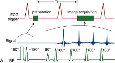
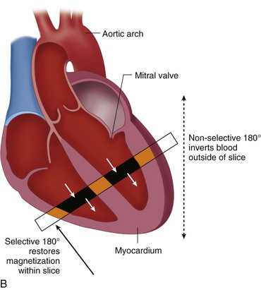
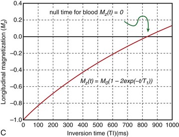
FIGURE 13-3 A, Pulse sequence diagram of a black blood FSE sequence showing details of the double IR magnetization preparation segment and the FSE image acquisition segment. B, The first nonselective IR pulse inverts the spins everywhere. This is immediately followed by a slice-selective inversion RF pulse that reinverts or restores the perturbed magnetization only in the imaged slice. Following an interval TI, uninverted blood has exited the slice and is replaced by inverted blood. C, By choosing the TI time such that the longitudinal magnetization of blood is zero, blood signal within the imaged slice is suppressed.

Typical image acquisition parameters for a black blood FSE acquisition are a 256 × 192 acquisition matrix with an ETL = 20 and two R–R intervals per acquisition segment; this translates to an approximate breath-hold time per slice of about 20 seconds (assuming 60 beats/min heart rate). Complete coverage of the heart using black blood FSE requires about 8 to 12 slice locations with separate breath-holds at each location. To further improve the efficiency of the black blood FSE acquisition, the inversion and image acquisition can be compacted into a single R–R interval (e.g., FSEuno). By removing the time for recovery of the longitudinal magnetization in the second R–R interval, increased T1-weighting is also achieved. Additionally, the acquisition of four slices in the same time as a single slice in a conventional two R–R interval gated FSE pulse sequence (e.g., FSEquatro) can be realized by grouping adjacent slice locations together.¹³ As shown in Figure 13-4, two slice locations are acquired in each R–R interval (for four slices in total for a two R–R interval acquisition). Because the slices are adjacent to each other, the slice-selective reinversion RF pulse now spans two slice locations providing blood suppression for both slices. The number of breath-holds for whole heart coverage is reduced by a factor of 4 (Fig. 13-5), significantly speeding up the cardiac examination and reducing patient fatigue from frequent and repeated breath-holds.

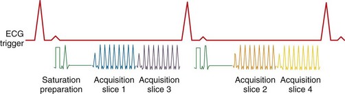
FIGURE 13-4 Diagram illustrating how four slice locations can be acquired in a single acquisition by interleaving. Because each R–R interval has a nonselective IR pulse (from the double-IR saturation preparation at the start of systole) that affects spins over the entire heart, there is less time for recovery of M_z in the imaged slice in segmented k-space acquisitions. The images have a stronger component of T₁ weighting than conventional two R–R black blood imaging sequences. Referred to as FSEquatro, this type of acquisition sequence significantly reduces the overall scan time.

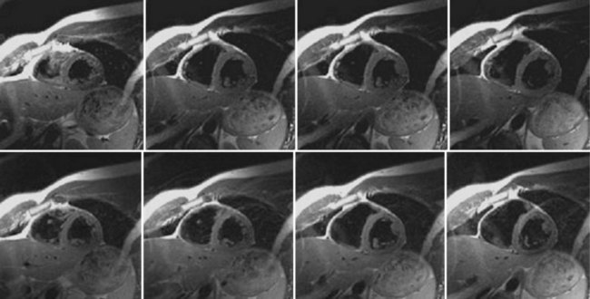
FIGURE 13-5 Comparison between a multislice study using FSEquatro (top row) and conventional FSE (bottom row). The FSEquatro scheme acquired four slice locations in a single 22-second breath-hold (ETL = 16), whereas the conventional two R–R FSE could acquire only one slice location per breath-hold. Overall, the conventional two R–R FSE acquisition took 4 minutes, allowing the patient to rest between breath-holds. Image quality between the two approaches is equivalent, emphasizing the improved efficiency of current black blood FSE imaging developments.

Myocardial Perfusion

Myocardial perfusion imaging identifies regions where there is a blood flow deficit in the myocardium by tracking the first pass of a contrast medium bolus over several cardiac cycles. This tracking requires the use of a fast imaging pulse sequence that repeatedly acquires an image every one to two R–R intervals over 30 to 40 seconds, with sufficiently high image contrast to delineate regional differential uptake of contrast medium. In addition, any changes in image contrast over time must be due only to changes in concentration of the contrast medium in the tissue, and must be immune to variations in heart rate.

To achieve robust image contrast, a 90-degree saturation recovery magnetization preparation segment, followed by a fixed time TI, is used for myocardial perfusion studies. A 90-degree rather than a 180-degree preparation RF pulse is used because the longitudinal magnetization recovers from the same level (M_z = 0) during the TI interval for each ECG-gated acquisition during the contrast uptake. With saturation recovery magnetization preparation, the tissue signal intensity is independent of the cardiac R–R interval, eliminating signal variations caused by arrhythmia (Fig. 13-6). The relatively short TI time (100 to 200 ms) of the saturation recovery preparation pulse suppresses signals from long T1-weighted tissues, such as the unenhanced myocardium and blood, while emphasizing tissues with markedly reduced T1 times from contrast medium uptake. With the correct selection of acquisition parameters and contrast medium dose, saturation recovery magnetization preparation can yield signal intensity changes that are linear with contrast medium concentration, providing an opportunity for quantitative assessment of myocardial perfusion.

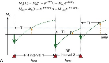
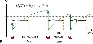
FIGURE 13-6 A, Variation in signal intensity, given as M_z(TI), with IR preparation. The signal intensity is a strong function of the longitudinal magnetization at the end of each R–R interval (t_RRn). If the patient’s heart rate varies during the myocardial perfusion acquisition, there is a strong variation in signal intensity depending on the heart rate changes. B, In contrast, if a saturation recovery preparation is used, the signal intensity depends only on the TI time, and is immune to variations in the patient’s heart rate. The solid triangles indicate the time of a detected cardiac trigger and the point in time when the magnetization preparation pulse is applied. is defined as the longitudinal magnetization just prior to the application of the IR pulse in RR interval n (i.e., the longitudinal magnetization at the end of RR interval (n − 1).

To achieve full coverage of the left ventricle during the first pass of the contrast medium, it must be possible to fit an optimal number of acquisition segments (with each segment consisting of the magnetization preparation pulse, TI interval, and data acquisition section) into either one or two R–R intervals. The TI interval section and the data acquisition segment can be optimized to provide the shortest possible time with best possible image quality. Although single-shot EPI (all k-space lines acquired after a single RF excitation pulse) has poor image quality for cardiac perfusion studies, a segmented and interleaved approach accomplishes short scan time and good image quality.^14–16 In interleaved EPI, only a few echoes per RF excitation pulse (ETL = 4) are used, resulting in short (6 ms) TR times; this yields an acquisition approach with high efficiency (time per echo). With improvements in gradient hardware, however, fast gradient echoes (and balanced SSFP) with an ETL = 1 and TR = 2 ms or less have also yielded images with comparable image quality and with equal compactness in time.^17–19

Effective assessment of myocardial perfusion defects requires maximal tissue contrast, which is obtained from an optimal TI time at typical contrast medium doses of 0.05 to 0.10 mmol/kg.²⁰ To maximize the number of slice locations that can be acquired per R–R interval, however, the time for each acquisition segment needs to be as compact as possible. By minimizing the TI time, more slice locations can be acquired per R–R interval; however, this leads to compromises in image contrast because there is an inherent tradeoff between TI and image contrast-to-noise ratio (CNR). Several approaches allow for significantly reduced TI times, while maintaining sufficient tissue contrast. By interleaving the saturation recovery RF pulse and image acquisition using a slice-selective notched saturation, longer TI times can be achieved with minimal dead times.²¹ Alternatively, the center of k-space in the image acquisition section can be reordered to the end of the acquisition segment, yielding a longer “effective” TI time. Both approaches produce satisfactory image contrast with as compact an acquisition segment as possible.

Sections of the myocardium where there is a regional perfusion deficit are hypointense relative to the normal myocardium because of reduced uptake of contrast medium. By a qualitative assessment of signal intensity changes, myocardial perfusion deficits can be easily identified (Fig. 13-7). A troubling artifact with myocardial perfusion using MRI is the so-called “dark rim” artifact, which is characterized by a transient and distinct hypointense thin region in the endocardium that mimics a perfusion defect (Fig. 13-8).²² This phenomenon usually occurs immediately after the contrast medium bolus first arrives in the left ventricle, but does not persist over time. Improvements in spatial resolution and substantial reduction in image acquisition times reduce the occurrence of these artifacts, as does requiring positive identification of a defect that spans several slices and persists through multiple frames of the scan.

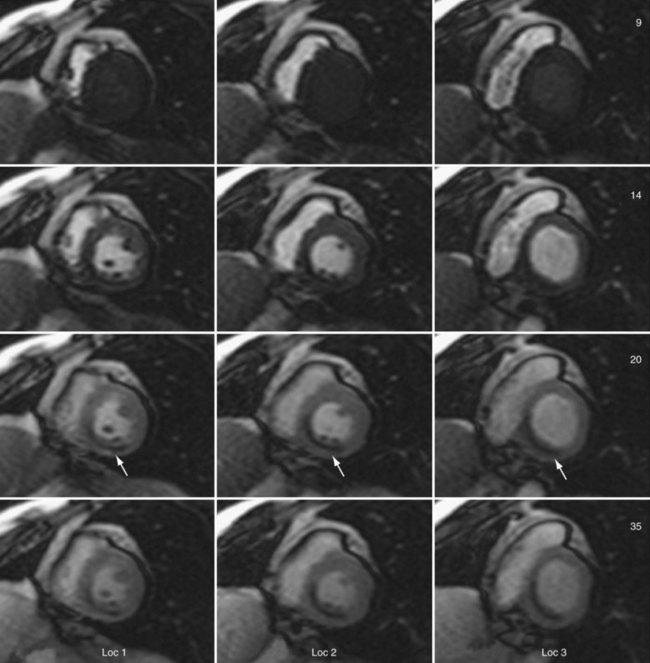
FIGURE 13-7 Example of a fixed perfusion defect in a patient with a known inferoseptal wall myocardial infarction (arrow). Three short-axis slices are shown at different time points (each row) following a 0.10-mmol/kg contrast bolus. A persistent region of hypointensity observed is indicative of a perfusion deficit and was evident over 20 frames. With a two R–R acquisition, each frame (number) represents two heartbeats.

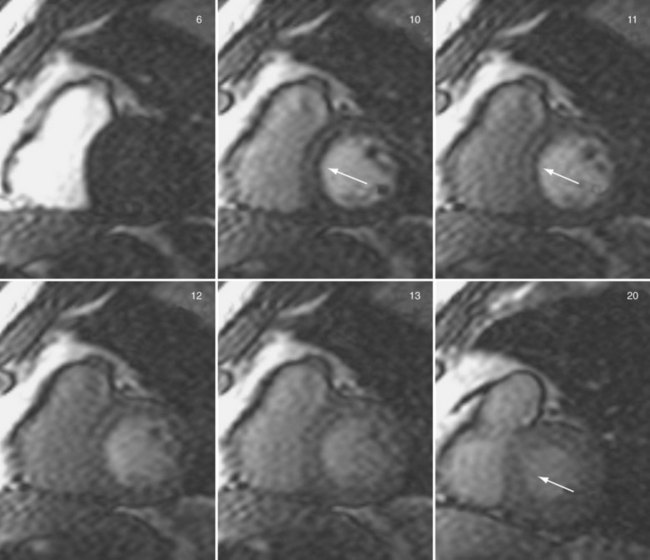
FIGURE 13-8 Dark rim artifact (arrow) mimicking a perfusion defect as shown in an interleaved EPI pulse sequence with ETL = 4 and 128 × 128 acquisition matrix. This example shows 6 frames from a 30-frame acquisition. The artifact is evident in frames 10 and 11 during the first pass of the contrast bolus through the myocardium. This dark rim rapidly diminishes in subsequent heart beats (frames 12 and 13) and is completely absent in frame 20. Nonpersistent regions of hypointensity that do not span several slice locations are generally classified as image artifacts and are ignored.

Myocardial Viability

Myocardial delayed enhancement (MDE) imaging provides an accurate method for determination of myocardial viability.^23,24 On first-pass perfusion imaging, infarcted myocardial tissue does not enhance after gadolinium-chelate contrast agent administration because of its restricted blood flow. Over time, the gadolinium-chelate contrast agent diffuses into the infarcted region. The poor vascular supply to the infarcted region is associated with diminished washout of contrast agent. Infarcted tissue exhibits delayed gadolinium uptake and delayed washout. Normally perfused myocardium has much faster early uptake and brisk washout. Delayed imaging of the left ventricle (beginning 5 to 10 minutes after contrast agent administration) enables optimal differentiation of infarcted from noninfarcted (i.e., normal) myocardium. On delayed imaging, infarcted myocardium appears more enhanced (i.e., “hyperenhanced”) relative to that of normal enhancing myocardium (T1 shortening).

The best technique for visualizing delayed hyperenhancement is an IR GRE pulse sequence that suppresses signal of the normally enhancing myocardial tissue, while maximizing the signal difference with that of the hyperenhancing infarcted tissue.²⁵ To maximize the image contrast between normal myocardium and hyperenhancing infarcted tissue, the TI time is selected to null normal myocardial signal during the acquisition of the central k-space view. Because hyperenhancing infarcted tissue has a higher concentration of gadolinium contrast agent, it has a substantially shorter T1 time (approximately 75 ms) relative to normal myocardium (approximately 290 ms). Nulling the signal from normal myocardium yields a high contrast image differentiating the bright infarcted regions from the dark background. The primary image acquisition technique is an ECG-gated, segmented k-space, two-dimensional acquisition where each slice is acquired in a single breath-hold (Fig. 13-9), requiring multiple breath-holds for complete coverage of the left ventricle.

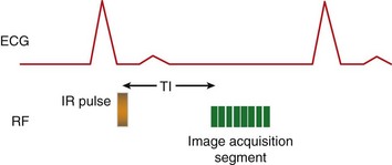
FIGURE 13-9 Diagram illustrating MDE acquisition. The image acquisition section is an ECG-gated segmented k-space gradient-echo pulse sequence that follows a nonselective IR RF pulse. Typically, 20 k-space lines are acquired in each cardiac interval. The subsequent R–R interval either can be repeated for signal averaging or can be used to allow for a more complete recovery of the longitudinal magnetization.

Although a temporal resolution of about 40 to 50 ms is usually targeted in cine imaging to best visualize motion over the whole cardiac cycle, MDE imaging is able to tolerate temporal resolutions of 150 ms without significant cardiac motion degradation. The number of vps can be substantially increased over a cine scan (see Equation 1), shortening the overall scan time. Typical image acquisition occurs in mid-to-end systole or at a delay of 300 to 400 ms from the cardiac R wave.

To improve image CNR, there are two approaches. With a two R–R interval approach, image acquisition occurs in the first R–R interval, and the second R–R interval is used for more complete magnetization recovery.²⁴ An alternative approach is a single R–R acquisition with double the number of excitations. In the latter approach, there is less time for longitudinal magnetization recovery, but by doubling the number of signal averages, some reduction in motion-related artifacts is realized. In both schemes, the overall scan time is the same, where one slice location is acquired in a single breath-hold.

Maximizing image CNR between normal and infarcted myocardial tissue requires a judicious choice of TI times. As noted in Figure 13-10, the contrast at different TI times varies according to whether phase-sensitive inversion recovery (PSIR) or magnitude IR is used. With PSIR, the signal phase is preserved, allowing for negative values of signal intensity (i.e., to account for negative signal intensities when the longitudinal magnetization is <0).^26,27 In magnitude IR, phase information is lost, and all signal intensities are positive (>0). PSIR and magnitude IR provide identical tissue contrast for TI > t_null,myo, the null point for normal myocardium. The advantage in PSIR occurs when TI is significantly shorter than t_null,myo, where contrast is maintained between normal and infarcted myocardium, whereas in magnitude IR, contrast diminishes and inverts if the TI time is decreased further. Although PSIR is less sensitive to TI times when TI < t_null,myo, there is no benefit if TI ≥ t_null,myo. The optimum TI must still be determined for maximum contrast to avoid setting too long a TI time.

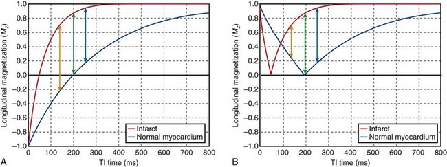
FIGURE 13-10 A and B, Plot showing the evolution of longitudinal magnetization of normal myocardium (TI = 290 ms) and infarcted tissue (T₁ = 75 ms) with a phase-sensitive IR (A) and magnitude IR (B) acquisition. As shown in this example, the optimum TI time is at TI = 200 ms, and results in maximum contrast between normal and infarcted myocardium. For TI greater than the optimum TI time (TI > 200 ms), contrast for phase-sensitive IR and magnitude IR is identical. For TI times less than the optimum time (TI < 200 ms), contrast in phase-sensitive IR is maintained, whereas contrast for magnitude IR is diminished. This is because the signal phase is preserved in the phase-sensitive image, whereas magnitude IR has signal intensities greater than zero only. Subsequently, inversion of contrast is possible for short TI times.

The optimal TI time can be chosen by performing repeated test scans at several different TI times; this can be time-consuming because each acquisition requires a separate breath-hold. As contrast medium concentrations diminish over time, the optimal TI time also changes as a function of time after contrast injection. Alternatively, the appropriate TI time can be determined using a scout acquisition that acquires images at different TI times in a single acquisition. By selecting the best image that has complete suppression of normal myocardium, the corresponding TI time can be used in the MDE acquisition. One such TI scout technique uses a GRE cine pulse sequence with an IR pulse applied immediately at the cardiac R wave trigger.^28,29 This cine IR approach reconstructs images at different times from the IR pulse where each cardiac phase represents a different TI time. Images at multiple TI times can be obtained in a single breath-hold acquisition to choose the appropriate TI time (Fig. 13-11).

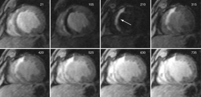
FIGURE 13-11 cine IR images acquired in a single acquisition at equivalent TI times of 21 ms, 105 ms, 210 ms, 315 ms, 420 ms, 525 ms, 630 ms, and 735 ms. This approach acquires 40 phases, with each phase at a different TI time from the IR pulse. By inspecting the reconstructed images, the optimal TI time can be selected and used for the high spatial resolution acquisition. In this case, TI = 210 ms results in maximal suppression of the normal myocardium and high contrast of the large septal infarct (arrow) in this patient. At TI < 210 ms, there is an inversion of contrast (dark infarct) in this magnitude reconstruction. At TI > 210 ms, there is reduced contrast as the longitudinal magnetization of the normal myocardium and infarct approach similar thermal equilibrium values.

As with a two-dimensional cine scan, an MDE study can be challenging for a patient because of repeated breath-holding. Single-shot methods using shorter TR gradient-echo or balanced SSFP have longer acquisition windows, but allow multiple slice locations to be acquired in a single breath-hold or in a series of much shorter breath-holds.^30,31 Compared with a conventional MDE study where the acquisition window of 120-150 ms per cardiac cycle is used, single-shot techniques use acquisition windows in the range of 220 to 250 ms. In addition, a much shorter TR with higher receiver bandwidth leads to a reduction in image CNR. By using approximately the same acquisition window per R–R interval, the MDE study can be extended to a three-dimensional acquisition where a SNR advantage is realized (where n is the number of slice partitions in the volume scan).^32–34 By trading off some increased motion blurring (that does not compromise diagnosis) against higher SNR, the efficiency of the myocardial viability study can be improved. In addition, variations that include fat suppression allow for assessment of specific patterns of hyperenhancement as may be seen in arrhythmogenic right ventricular dysplasia.³⁵

Tagging and Wall Motion Assessment

Although cine MRI allows the assessment of wall motion by visualizing global myocardial contractility, MRI also has the ability to measure regional myocardial wall function directly. The basic approach is to set up a series of grid lines at the start of systole using a magnetization preparation segment consisting of nonselective RF pulses and gradient pulses, and to follow the evolution of these tagged lines through systole.^36,37 Tag lines in the image are applied using a tagging sequence as shown in Figure 13-12. In a simple view with a two-RF pulse tagging sequence, the first RF-excitation pulse tips into the transverse plane all spins within the coil volume. The gradient pulse causes the spins to acquire a relative phase as a function of position. At some time τ, a second RF pulse restores the longitudinal magnetization except for the spins that are aligned along the x′-axis in the rotating frame. Spatial locations that have acquired a relative phase where φ = π/2, 3π/2, … , (2n + 1)π/2 will have minimal signal (φ = , where is the magnetic field gradient, is the position, τ is the gradient waveform pulse width, and γ is the gyromagnetic ratio).

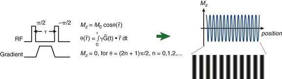
FIGURE 13-12 Diagram illustrating a simple tagging sequence. The two RF excitation pulses and intervening gradient waveform generate a sinusoidally varying intensity in the image. The dark lines in the image correspond to M_z = 0. Better definition of the tag lines can be achieved by using more RF pulses.

Because only the component of the transverse magnetization that is perpendicular to the direction of the applied RF excitation field (x′-axis) is restored by the second RF pulse to the longitudinal axis, a range of signal intensities according to position is generated by the tagging sequence. The signal intensity varies as:

(6)

This results in a sinusoidal variation of signal intensity according to position. Two-dimensional grid tags can easily be applied by first applying the tagging sequence in one direction, followed by the same tagging sequence but with a gradient field in an orthogonal direction. The tag lines can also have better definition (sharpness) by increasing the number of RF pulses and corresponding gradient pulses, and varying the relative amplitudes of the component RF pulses.³⁸ The tag separation can be controlled better with an increased number of RF and gradient pulses in the tagging sequence.

As the tagged regions evolve over the cardiac cycle, normal myocardial wall motion is seen as a contraction of the pattern of grid lines in systole, followed by separation or relaxation in diastole (Fig. 13-13). Nonfunctioning sections of the myocardium exhibit no such contractility. Quantitative assessment of myocardial strain is possible from analysis of the deforming tag lines. More efficient techniques have been introduced that allow faster computation of myocardial strain by analyzing the phase evolution of the tag lines in k-space.^39,40

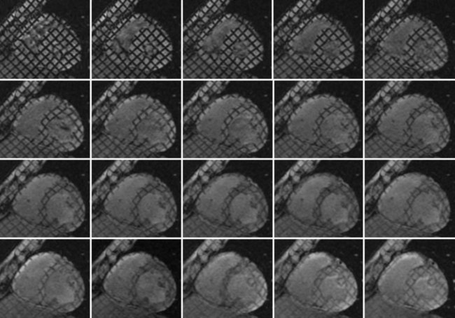
FIGURE 13-13 Twenty phases from a segmented k-space tagging sequence in a healthy volunteer at 3.0 T. In this example, a two-dimensional tagging grid is applied at the cardiac R wave. As the heart contracts in systole and dilates in diastole, the deformation of the regular grid pattern is evident. Uniform deformation of the myocardial tagging grid of the left ventricle is indicative of normal wall motion and function.

Coronary Artery Imaging

Developments in navigator technology and faster acquisition pulse sequences have resulted in substantial progress in using MRI for coronary artery stenosis assessment. Coronary artery imaging methods can be divided into whole heart imaging⁴¹ and targeted oblique acquisitions.^42,43 In the latter technique, the volume (three-dimensional) acquisition is targeted to specific vessels. Typically, to image the left main coronary artery, left anterior descending coronary artery, right coronary artery, and left circumflex coronary artery, three separate acquisitions are required. For whole heart imaging approaches, the entire heart is imaged in a single acquisition, followed by segmentation of the coronary arteries using postprocessing algorithms available on image analysis workstations.

Short breath-hold three-dimensional techniques^42,44 are most suitable for the targeted approach. With breath-hold times of 20 to 28 seconds, an oblique three-dimensional volume encompassing the coronary artery can be easily and rapidly acquired. Three targeted, breath-hold coronary three-dimensional MR angiography acquisitions that include the left main and proximal segments of the left anterior descending coronary artery, right coronary artery, and left circumflex coronary artery are typically imaged within 5 minutes, assuming the patient is able to tolerate repeated breath-holding. The short scan times allow the coronary artery assessment to be completed immediately after the first-pass perfusion study and before performing the myocardial viability assessment.

Because most patients with cardiac disease are unable to tolerate long breath-holds, free-breathing or respiratory-navigator techniques are employed.⁴⁵ In navigator imaging of the coronary arteries, the position of the diaphragm is monitored before data acquisition in each R–R interval. The navigator acquisition is a two-dimensional slice selective column that is prescribed typically over the right hemidiaphragm in the cranial-caudal direction. The right hemidiaphragm is chosen for tracking diaphragmatic excursion because the lung-liver interface provides an excellent tissue-contrast interface. The placement of the tracker in the right hemithorax places the dark saturation bands related to navigator gating away from the heart. In each R–R interval, the profile along the navigator column is measured and analyzed to track the displacement of the lung-liver interface. A training phase is usually performed to determine automatically the end-expiration position; this is used as a reference profile (Fig. 13-14). During the navigator scan, a least-squares determination of the displacement of the measured profile is made relative to the reference profile (end-expiration). If the position falls within an acceptance window around the end-expiration position, the data are accepted. If not, the same k-space encoding views are repeated until the diaphragm position is noted to fall within the acceptance criteria.⁴⁶

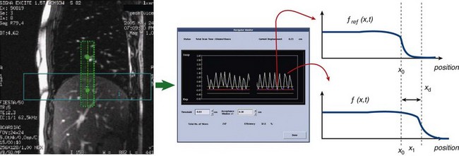
FIGURE 13-14 Principle of navigator-echo gating. A two-dimensional selective excitation is made in the cranial-caudal direction over the right hemidiaphragm.

From the projection along the excitation column, an edge detection algorithm detects and displays the position of the diaphragm as a function of time (center plot). The displacement relative to a reference position, x_d, is measured using a least-squares fit. From these data, the end-respiratory position (red line) can be displayed. If the diaphragm position falls within the acceptance window of the end-respiratory position, the data are accepted.

Let f_ref(x₀) be the profile along the navigator column that represents the mean end-expiratory position, where x₀ is the reference position in mm. To determine the displacement at time t, the corresponding navigator profile is f(x′,t), where x′ denotes position of the navigator profile at time t. The relative displacement of x′ from x₀ is determined by varying x_d over a range of values such that:

(7)

where x_d is the displacement of the profile from its measured position. The value of x_d is the displacement of the subject navigator profile from the reference profile. This value is plotted as a function of time (as shown in Fig. 13-14) in real time either to accept or to reject that acquisition view.

Specifically for coronary artery imaging, the navigator segment must be integrated with the data acquisition segment and a fat suppression segment (Fig. 13-15). Fat suppression is required because the coronary arteries are embedded in epicardial fat that yields high signal intensities similar to that of blood. The navigator gating sequence synchronizes image acquisition for end-expiration, and enables the extension of the imaging window over many respiratory cycles for improved high spatial resolution, whole heart imaging of the coronary arteries. From the three-dimensional volume, planar reformations or surface rendering can better depict long lengths of the coronary artery.⁴⁷

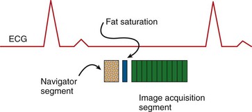
FIGURE 13-15 Navigator-echo gating in a segmented acquisition. In each cardiac R–R interval, a navigator segment is played out followed by the fat suppression magnetization preparation segment and the data acquisition segment. The sequence is repeated until all necessary data for the three-dimensional volume acquisition are acquired.

Free-breathing techniques have disadvantages. In practice, the shorter the scan time, the greater the chances that the scan is successful. There is a normal drift in the location of the diaphragm over time⁴⁸ that changes the end-expiration position, resulting in poor performance of the navigator compensation. If the scan time can be shortened (e.g., using parallel imaging), the probability of diaphragm drift can be reduced, improving the image quality. The ongoing development of coronary artery imaging techniques has focused on minimizing the effects of cardiac and respiratory motion, primarily by reducing the overall acquisition time, but also by determining the optimal quiescent period of the heart when there is minimal motion.

Phase Contrast Imaging

In addition to excellent soft tissue visualization, MRI affords the ability to quantify flow in a manner similar to Doppler ultrasonography, but without the restrictions of limited acoustic windows. Phase contrast angiography^49–51 discriminates between flowing spins and stationary tissue by measuring differences in accumulated phase in the direction of a flow-sensitizing gradient. Phase contrast data can provide the velocity of flowing spins (i.e., flowing blood) and the direction of blood flow.

If we consider a magnetic field gradient applied in a specific direction, the phase accumulated by an ensemble of spins moving with a constant velocity, , in that direction is:

(8)

where describes the time-varying gradient (direction and amplitude), γ describes the gyromagnetic ratio, and r₀ describes the initial position of the spins. The terms M₀ and M₁ represent the zero and first moments of motion of the spins in the gradient field. If we follow this first gradient waveform with a second waveform that is identical but of opposite polarity, the accumulated phase is then:

(9)

where represents the first gradient moment from the combined bipolar gradient waveform. The phase accumulation from this bipolar gradient waveform (Fig. 13-16) arises only from flowing spins, with the contribution from stationary spins (the r₀ component) canceled out by the gradient lobes of equal amplitude but opposite polarity. Only flowing spins contribute to nonzero phase accumulation, the magnitude and sign of which are directly related to the velocity and direction of flow.

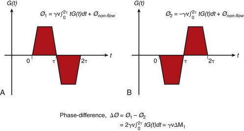
FIGURE 13-16 A, Bipolar flow-sensitizing gradient waveform. Because the second lobe is identical but of opposite polarity to the first gradient lobe, accumulated phase from stationary spins (i.e., protons) is zero, and the remaining nonzero accumulated phase is due only to motion (moving protons such as flowing blood). However, there may be nonzero phase from nonflow-related sources (Ø_nonflow). B, When a second acquisition is performed with the polarity of the bipolar gradient reversed, the phase from nonflow-related sources is unchanged, but the phase arising from blood flow is the negative of the phase from the first acquisition. Taking the phase difference between the two acquisitions, the nonflow-related phase is canceled, leaving only the phase that is due to blood flow.

A single acquisition with a bipolar flow-sensitizing gradient ideally provides an image whose phase represents flow in the direction of the applied gradient as given by Equation 9. Residual eddy currents, magnetic field inhomogeneity, and miscentering of the MRI echo in the acquisition window contribute to a spatially varying nonzero phase unrelated to flow or motion (Fig. 13-17A and B). To overcome this problem, two images with bipolar gradients of opposite sign (toggled bipolar gradients) are subtracted. Any nonzero phase in stationary tissue is canceled out, leaving an image with the phase difference accumulated in the two acquisitions owing only to flow (Fig. 13-17C). The phase difference (ΔØ) from the toggled bipolar flow gradient is then:

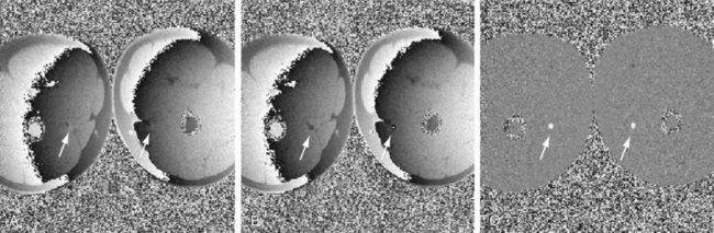
FIGURE 13-17 A, Axial phase image of the thighs of a healthy volunteer with a flow-sensitizing gradient applied in the cranial-caudal direction. A spatially varying nonzero phase is observed in the stationary tissue and the arterial and venous structures. B, Axial phase image of a second acquisition, but with the polarity of the flow-sensitizing bipolar gradient reversed. Signal in the femoral arteries is now negative (arrows) relative to the first acquisition (A), but the background phase is unchanged. C, Taking the phase difference between the two acquisitions cancels out the nonzero phase unrelated to flow, leaving the phase signal in the femoral arteries clearly depicted. The phase of the stationary background tissue is now zero.

(10)

with:

(11)

where G(t) is the bipolar gradient waveform.

The phase contrast approach to velocity imaging can be applied to cine pulse sequences (see Figs. 13-1 and 13-2) to generate ECG-gated images that depict flow velocities in the heart and blood vessels as a function of the cardiac cycle. With phase contrast cine images, the magnitude and direction of intracardiac shunts and valvular dysfunction (Fig. 13-18) can be easily observed. It is also possible to compute net flow (integrated over the entire cardiac cycle) through vessel cross sections (Fig. 13-19), and the forward and reverse components of flow. Phase contrast cine is an essential tool for flow quantification in patients with atrial septal defects or similar congenital cardiac disease where the measurement of regurgitant volumes or shunt flow is required.^52,53

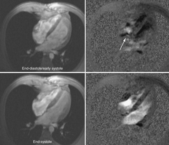
FIGURE 13-18 Cine phase contrast MRI. Magnitude (left column) and phase (right column) four-chamber images from a cine phase contrast examination in a patient with tricuspid insufficiency. The acquisition was acquired with flow sensitivity in the right-left, anteroposterior, and superoinferior directions. Only the right-left phase-velocity image is shown. There is black flow (arrow) on the four-chamber phase velocity map image (top right image) signifying left-to-right flow (i.e., regurgitant) into the right atrium during systole; it cannot be seen in the magnitude image. Antegrade flow through the tricuspid valve is seen during diastole as white (bright) signal signifying right-to-left flow direction on the diastolic phase velocity map (bottom right image). Direction of blood flow is encoded as either bright or black pixels based on flow direction. On a right-left phase velocity map, right-to-left flow is bright; left-to-right flow is black.

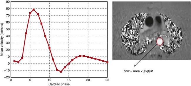
FIGURE 13-19 Measurement of mean flow velocities across a cross-sectional area of the descending aorta as a function of cardiac phase in a cine phase contrast examination. The net flow is computed by integrating the velocity-time curve over the cardiac cycle and multiplying this by the measured cross-sectional area of the vessel.

Fast Pulse Sequences

A primary method for speeding up imaging of the heart has been the adoption of faster pulse sequences. The first of these to be developed, the echo-planar imaging (EPI) sequence,¹ executes a raster pattern back and forth across all of raw-data space, or “k-space,”⁵ after a single RF excitation. This is in contrast to conventional acquisition approaches that acquire a single line of k-space data per excitation (Fig. 13-20). Although this sequence dates from the earliest days of MRI, it did not become practical for cardiac imaging until the advent of improved gradient hardware.^3,54 This improved hardware has also enabled real-time⁵⁴ EPI movie loops and high-quality phase contrast interleaved EPI images¹⁵ of the heart. Interleaved EPI pulse sequences,^14,15 which employ multiple excitation pulses with interleaved k-space trajectories, were developed later to reduce the ETL, and minimize some of the artifacts associated with EPI sequences.

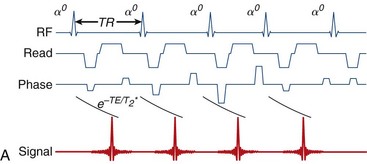
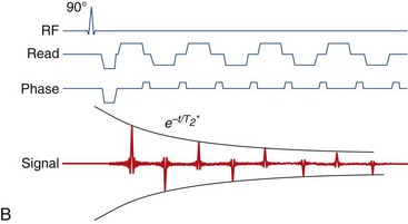
FIGURE 13-20 A, Conventional gradient-echo acquisition where one echo or k-space line is acquired per RF excitation pulse. To maintain higher SNR, a low flip angle (α < 90 degrees) is used. B, In contrast, EPI acquires multiple echoes for a single RF excitation pulse. The gradient echo is refocused multiple times by gradient reversal, allowing multiple k-space lines to be acquired, increasing the acquisition efficiency. The echo amplitudes in an EPI train are modulated, however, by T₂* decay.

Improvements in gradient hardware also benefited another class of fast imaging sequence, balanced SSFP.^8,55 This method relies on balanced gradient waveforms and short TR to rewind coherently the magnetization after each readout, and avoid signal saturation effects that degrade other short TR sequences. Balanced SSFP images are characterized by relatively high SNR and bright blood signal, but require TR on the order of 3 ms or less (at 1.5 T) to avoid dark banding artifacts arising from off-resonance effects. The greater the inhomogeneity present, the shorter the TR times required.

Another class of imaging sequence replaces rectilinear k-space trajectories with curved paths that push the gradient slew rate (which can be viewed as the rate of change of motion along the trajectory) more evenly over the entire sequence. The most successful of these arguably has been the spiral trajectory^5,6 and its variants. The spiral trajectory can be traversed at a nonuniform angular rate to produce constant gradient amplitudes or slew rates, and maximize bandwidth.⁵⁶ The advantages of reduced echo times gained by interleaving in EPI also hold for interleaved spirals. Spirals have the further benefits of good flow characteristics⁵⁷ and relative insensitivity to motion,⁵⁸ making them especially useful for cardiac imaging. Off-resonance and susceptibility effects can affect image quality, however, and measures such as automated field-map calculation and correction in the image reconstruction are generally necessary to prevent regional image blurring.⁵⁹

Parallel Imaging

The conventional approach to faster MRI pulse sequences, through reductions in the sequence TR time, is inherently limited by gradient amplitude and slew-rate constraints. These constraints arise partly from hardware limitations, but more fundamentally from the potential for peripheral nerve stimulation. A newer class of methods for speeding up MRI acquisitions, parallel imaging,^60,61 overcomes this limitation by shifting some of the responsibility for spatial encoding from the gradients to an array of RF receiver coils.⁶² This shift removes the dependence for shortening scan times on reducing TR by instead reducing the amount of data to be collected.

In parallel imaging, k-space is undersampled (reducing the overall data required to reconstruct an image) to improve imaging speed. Normally, undersampling k-space results in aliased images in which signals from different locations appear (erroneously) to originate from the same pixel. Because the signal from each location is uniquely weighted in each coil element (with each coil element having different spatial sensitivity patterns), however, this feature can be used to distinguish each location’s contribution to the aliased pixels, and unwrap the overlapping signals.

This method of undersampling k-space and using spatially arrayed RF coils to reconstruct artifact-free images is termed parallel imaging. Parallel imaging techniques fall into two classes: k-space-based techniques such as SMASH (simultaneous acquisition of spatial harmonics)⁶⁰ and GRAPPA (generalized autocalibrating partially parallel acquisitions),⁶³ and image-space–based methods such as SENSE (sensitivity encoding).⁶¹ These techniques typically use either a separate acquisition first to generate spatial sensitivity maps for each coil or autocalibration, in which the center of k-space is fully sampled within an undersampled acquisition, and low-resolution sensitivity maps are generated from that portion of the data.

Early application of parallel imaging to the heart used the SMASH method in coronary MRI, to bring a factor of 2 improvement to breath-hold times, spatial resolution, or time resolution.⁶⁴ Soon after this, SENSE imaging with a half-Fourier segmented EPI sequence was applied to breath-hold and real-time imaging to accelerate scanning by factors up to 3.2, resulting in low spatial resolution images in times as short as 13 ms using six-element cardiac phased-array coils.^65,66 Acceleration factors are constrained by the number of spatially arrayed coil elements. The higher the acceleration factor, the greater the undersampling of k-space data, and the greater the reliance on more coil elements for spatial encoding. Exceeding the threshold acceleration factor for the number of coil elements present leads to decreased ability to unwrap aliased pixels.

As channel counts increased, 32-coil torso⁶⁷ and cardiac⁶⁸ arrays were used for cardiac MRI, enabling acceleration factors of 16 for whole heart imaging. This development allows all three main branches of the coronary tree to be captured in a single breath-hold (Fig. 13-21). Arrays with higher channel counts have also brought improved image quality for accelerated real-time balanced-SSFP imaging at frame rates of 50 frames per second, potentially enabling improved stress testing.⁶⁹ An example of real-time cardiac imaging with a 32-channel cardiac array is shown in Figure 13-22. Channel counts have since continued to increase beyond 32 to 128,^70,71 resulting in improved quality for highly accelerated breath-hold cardiac MRI. Cardiac imaging with 128 channels has been shown more recently to yield acceleration rates greater than 12 to 20.⁷² Although coil losses and electrodynamics considerations seem to indicate that we may be nearing the useful limits of channel count (at least for field strengths of 1.5 to 3 T), more work remains to be done to explore the best use of high-channel cardiac MRI.

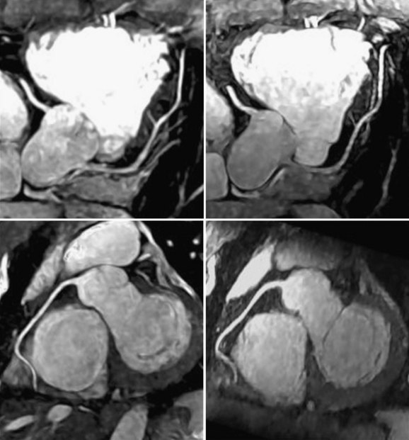
FIGURE 13-21 Planar angiographic reformations of left main and left anterior descending (top) and right coronary artery (bottom) using conventional thin targeted three-dimensional slab approach (matrix size 256 × 256 × 12) (left) and eightfold (4 × 2) accelerated three-dimensional parallel MRI of whole heart (right). With an increased number of channels (32), higher acceleration factors can be used, allowing significantly higher spatial coverage (matrix size 256 × 256 × 60) for the same imaging time as for a lower channel count MRI system.

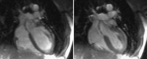
FIGURE 13-22 Diastolic and systolic frames from real-time balanced SSFP four-chamber data set acquired at 22 frames per second. This acquisition used a 32-channel cardiac phased array coil with an acceleration factor of 2 in a 128 × 72 matrix in a 33-cm field of view.

k-t Methods

In some cases, redundancies in the MRI signal acquired at different times in the cardiac cycle can be exploited to accelerate cardiac MRI effectively without the need for stronger gradients or multiple RF coils. In the earliest example of this, a sliding-window reconstruction was used to improve the effective frame rate of real-time fluoroscopic MRI.⁷³ In this method, as each new line (or group of lines) of k-space is acquired, it is combined with other, most recently acquired lines to compose a complete data set that is reconstructed to form an image for that point in time. In this way, the image reconstruction window is “slid” along in time, updating different parts of k-space at each new time point. Essentially, only a small but different portion of k-space is acquired at each time point, yielding a sparsely sampled k-t space (a data matrix with k-space along one dimension and time in the other). This method has also been applied to real-time cardiac MRI using interleaved spirals.⁵⁸

In a more recent development called UNFOLD (unaliasing by Fourier-encoding the overlaps using the temporal dimension), data from the dynamic object (the beating heart) are made to populate k-t space in a denser, more efficient manner.⁷⁴ Specifically, the data are undersampled by a factor of 2 and acquired in a time series where every odd image in the series uses a sampling function shifted in k-space by half of a line spacing compared with that used for the even images. After reconstructing each undersampled k-space data set at each time point (Fourier transformation in the k-dimension), this results in the signal intensity of aliased pixels alternating in position (shifted by half an image field of view) in each time frame, while unaliased pixels remain constant. When the time frames are played out as in a movie loop, the aliased pixels appear to flicker (i.e., change with high temporal frequency), whereas the unaliased pixels are steady (i.e., they exhibit only low temporal frequencies). After reconstructing the k-t data set to a series of images in time, this yields a pixel (x)-time (t) data set (or x-t data set).

The time series of images can be Fourier transformed in the time domain to generate plots of signal intensity at each pixel (x) versus temporal frequency (f) (i.e., resulting in an x-f space data set). Assuming that the temporal frequency distribution of the aliased and unaliased signals do not overlap, applying a low-pass filter removes the contribution of the high temporal frequency aliased signal, preserving the low temporal frequency unaliased signal. An inverse Fourier transformation back into the time domain (of the low-pass filtered x-f data set) returns flicker-free and unaliased time-series images. An image acceleration factor of 2 can be achieved even if only a single coil element is used. The amount of acceleration that is possible with this technique depends on the frequency spectrum of the cardiac motion. A wider range of cardiac frequencies indicative of the cardiac motion implies the need to use a wider bandwidth low-pass filter, limiting the maximum extent of undersampling. This is because for UNFOLD to work, the high temporal frequency distribution of the aliased pixels must be distinct and separate from the imaged object.

A more generalized k-t approach does not rely on such separation of temporal frequency data. This technique, called k-t BLAST (broad-use linear acquisition speed-up technique),⁷⁵ enables much higher acceleration factors than UNFOLD, while similarly not being constrained by the number of coil elements. The principle of k-t BLAST is simple. The time-series MRI data are uniformly undersampled in k-t space (i.e., different parts of k-space are collected at different times to form a sheared grid pattern—“quasi” diamond pattern—in k-t space). On Fourier transformation of this undersampled k-t data set, a replication of objects in the corresponding x-f space is obtained (i.e., pixels are aliased). Fully sampled data would yield x-f space that has fairly localized signal with noise everywhere else (i.e., pixels are not aliased). In the undersampled case, the object in x-f space is replicated throughout, and may overlap. This is in contrast to the case of UNFOLD, where the aliased or replicated objects do not overlap with the primary object. Because the replicated objects may overlap, the use of a low-pass filter as in UNFOLD would also remove data from the unaliased pixels. A much better method to remove the aliased pixels is needed.

The k-t BLAST technique uses a calibration scan or training data set to provide the necessary information to remove the aliased pixels in x-f space. By using a low spatial resolution fully sampled training data set (where there are no replicated objects), the areas of background noise in x-f space can be correctly identified to provide an expected background noise level. By comparing the expected noise level in each pixel in x-f space between that of the undersampled data set and the training data set, a reconstruction approach that minimizes the difference between the expected and measured noise levels effectively unwraps the aliased signals at each point in x-f space.

An inverse Fourier transformation back to k-t space yields an approximation of a fully sampled set that can be reconstructed normally to obtain alias-free images. In this manner, eightfold acceleration for cardiac imaging with reduced artifacts relative to a sliding-window reconstruction has been achieved without the use of multiple element phased-array coils.^75,76

Real-Time MRI

Rapid imaging pulse sequences are most useful when employed in the context of a system capable of high-speed reconstruction, real-time image display, and interactive scan-plane control. Such a setup was first developed and demonstrated by Wright et al.,⁷⁷ who used a workstation and array processor connected to a conventional MRI scanner. Other systems were developed later to enable real-time graphic control of the scan plane, or control by the use of three-dimensional hardware controllers.^78,79 Real-time interactive MRI systems have been applied to coronary MRI,⁸⁰ evaluation of left-ventricular function, MRI color flow,⁸¹ and interventional guidance,⁸² among other applications in the heart, and commercial real-time MRI systems are now widely available.

Because not all patients are able to maintain short breath-holds repeatedly over an extended time, real-time imaging provides an alternative that allows the completion of a cardiac examination with image quality sufficient for diagnosis. MRI system improvements, including faster imaging techniques and higher receiver channel counts, provide opportunities for real-time acquisition with significant advantages in temporal resolution, while improving spatial resolution. Real-time systems can also be essential enablers for new MR cardiac applications, such as pharmacologic or physical (e.g., bicycle or hand grip exercise) stress testing.

KEY POINTS

Methods for imaging the heart using MRI are described. Descriptions on how cine images of the heart can be obtained over several cardiac cycles, and the basics for acquiring images that provide information on myocardial viability, perfusion, and cardiac wall motion are provided.

In addition to soft tissue contrast, functional information can be obtained with MRI. Specifically, MRI is able to acquire images with information on the direction and velocity of flow. This information allows measurements of flow volumes and other physiologic indicators of cardiovascular disease.

Image acquisition times are currently longer than the periods of cardiac motion. Several cardiac cycles are required to acquire sufficient data to reconstruct images depicting the heart at different cardiac phases. Fast imaging techniques using parallel acceleration that reduce the k-space data requirements for image reconstruction have substantially sped up image acquisition. With a larger number of receiver coils, high acceleration factors permit real-time image acquisition with acceptable spatial resolution; this allows imaging with the patient breathing freely throughout image acquisition, rather than requiring repeated breath-holding.