CHAPTER 4 Magnetic Resonance Imaging of the Hip Joint
1 5-T Morphologic imaging
Examination Protocol
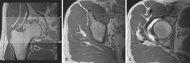
After a short localizer in three planes, the examination continues with an axial T1-weighted sequence (repetition time [TR] 650, echo time [TE] 20, 200 mm × 200 mm field of view, 224 × 512 matrix, 4-mm section thickness with a 0.2-mm section gap, 17 slices, 3 minutes and 44 seconds). The sequence is centered on the femoral head, and it covers the whole joint (Figure 4-1).
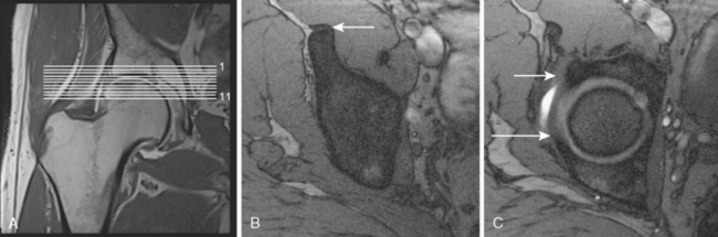
The second sequence is an axial FLASH sequence with a few thin slices that is centered on the upper joint space. This sequence is used to evaluate the version of the acetabulum, and it also helps with the assessment for subcortical hypersclerosis of the rim as well as for the presence of synovial cysts (TR 550, TE 10, flip angle of 90 degrees, 120 mm × 120 mm field of view, 256 × 256 matrix, 2-mm section thickness with a 0.1-mm section gap, 11 slices, 3 minutes and 6 seconds; Figure 4-2).
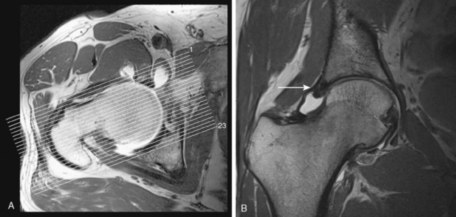
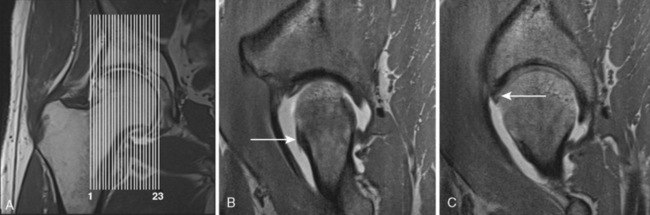
Next is a coronal–oblique proton-density l–weighted (PDW) thin-slice sequence (TR 3200, TE 15, 120 mm × 120 mm field of view, 256 × 256 matrix, 2-mm section thickness with a 0.1-mm section gap, 23 slices, 5 minutes). This sequence is aligned perpendicular to the femoral neck, and it is marked on the axial T1W sequence (Figure 4-3).
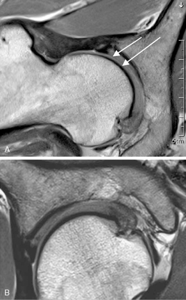
A second PDW sequence in the sagittal direction (TR 3200, TE 15, 120 mm × 120 mm field of view, 256 × 256 matrix, 2-mm section thickness with a 0.2-mm section gap, 23 slices, 5 minutes and 37 seconds) is applied as the next step (Figure 4-4).
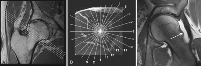
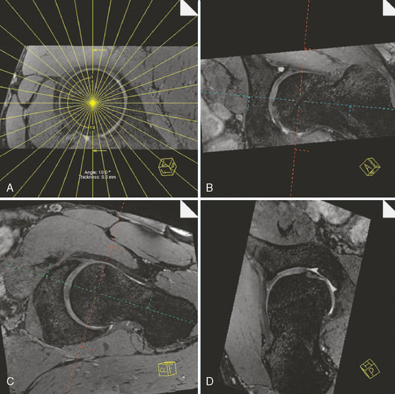
Finally, a radial PDW sequence (Figure 4-5) is used in which all slices are oriented basically orthogonal to the acetabular rim and labrum. This sequence is based on a sagittal oblique localizer, which is marked on the PDW coronal sequence, and it runs parallel with the sagittal oblique course of the acetabulum. The MRA imaging parameters are as follows: TR 2000, TE 15, 260 mm × 260 mm field of view, 266 × 512 matrix, 4-mm section thickness, 16 slices, 4 minutes and 43 seconds. In the center of the radial sequence, where the slices cross over, the signal wipes out. This produces a broad line without signal on the image, which affects the quality of the image. The more slices in a sequence, the broader the no-signal line gets. To reduce this artifact, this sequence is split into two sequences of eight slices each. The whole examination, including the hip injection, lasts about 50 to 60 minutes.
3-T Morphologic imaging
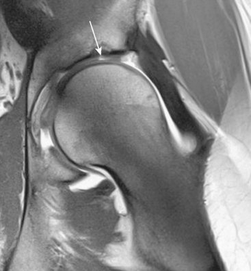
In addition to novel MR sequences, imaging quality can also be improved with the use of higher field strengths, because they provide a higher intrinsic signal-to-noise ratio, which is critical for high-resolution imaging. Two preliminary studies have been published about the use of 3-T imaging of the hip, which may help to improve the MR diagnostic accuracy of diagnosis with the use of high-resolution imaging. In addition, 3-T imaging may obviate the need for a contrast medium (Figure 4-6). The visualization of acetabular and femoral cartilage separation and the assessment of the acetabular labrum and adjacent cartilage—both of which are essential for an accurate diagnosis of FAI—can be improved with the use of high-resolution techniques. These advantages can also improve the usefulness of postoperative MR by monitoring cartilage integrity, which is a useful measure for evaluating surgical outcomes (Figure 4-7).
3-T Isotropic imaging
Isotropic three-dimensional sequences may provide for the diagnosis and characterization of acetabular and femoral cartilage on the basis of their anatomic correlation with the acetabular version or the femoral head–neck offset. A more precise overview of the different 3-T techniques is described in the review article by Philipp Lang, Farimah Noorbakhsh, Hiroshi Yoshioka. Figure 4-8 is an image from a patient with a cam-type impingement and cartilage degeneration with multiplanar reconstruction around the femoral neck that was obtained with the use of a three-dimensional true fast imaging with steady precession (FISP) sequence.
3-T Biochemical imaging
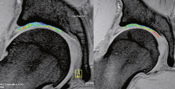
T2 mapping for biochemical imaging may be an alternative to the use of a contrast agent. T2 techniques make use of the T2 relaxation constant, which is affected by water–collagen interactions and, therefore, by water concentration, collagen concentration, and collagen alignment. In normal hyaline cartilage, there is a spatial variation of T2 with increasing values from the deep aspect to the superficial layer that are based on cartilage composition and structure within each layer. The influence of cartilage degeneration or alteration (e.g., cartilage repair tissue on the spatial T2 variation) has been investigated. The advantage of T2 mapping is that it does not require the use of a contrast agent. The drawbacks, however, are the nonspecificity of T2, as described previously, and the relatively long acquisition times required for the long echo trains needed for accurate T2 decay assessment (Figure 4-9).
Annotated references and suggested readings
Ganz R., Beck M., Leunig M., Nötzli H., Siebenrock H. Femoro-acetabuläres impingement. In: Wirth C.J., Zichner L., editors. Handbuch der Orthopädie. Stuttgart, New York: Thieme, 2003.
Ganz R., Parvizi J., Beck M., Leunig M., Nötzli H., Siebenrock K.A. Femoroacetabular impingement: a cause for osteoarthritis of the hip. Clin Orthop Relat Res. (417); 2003:112-120.
Ito K., Minka M.A.2nd, Leunig M., Werlen S., Ganz R. Femoroacetabular impingement and the cam-effect. A MRI-based quantitative anatomical study of the femoral head-neck offset. J Bone Joint Surg Br.. 2001;83(2):171-176.
Jager M., Wild A., Westhoff B., Krauspe R. Femoroacetabular impingement caused by a femoral osseous head-neck bump deformity: clinical, radiological, and experimental results. J Orthop Sci.. 2004;9(0):256-263.
Kim Y.J., Jaramillo D., Millis M.B., Gray M.L., Burstein D. Assessment of early osteoarthritis in hip dysplasia with delayed gadolinium-enhanced magnetic resonance imaging of cartilage. J Bone Joint Surg Am.. 2003;85-A(10):1987-1992.
Leunig M., Beck M., Kalhor M., Kim J., Werlen S., Ganz R. Fibrocystic changes at the anterosuperior femoral neck: prevalence in hips with femoroacetabular impingement. Radiology.. 2005;236(1):237-246.
Leunig M., Podeszwa D., Beck M., Werlen S., Ganz R. Magnetic resonance arthrography of labral disorders in hips with dysplasia and impingement. Clin Orthop Relat Res. (418); 2004:74-80.
Leunig M., Werlen S., Ungersbock A., Ito K., Ganz R. Evaluation of the acetabular labrum by MR arthrography. J Bone Joint Surg Br.. 1997;79(2):230-234.
Locher S., Werlen S., Leunig M., Ganz R. [Inadequate detectability of early stages of coxarthrosis with conventional roentgen images]. Z Orthop Ihre Grenzgeb.. 2001;139(1):70-74.
Locher S., Werlen S., Leunig M., Ganz R. [MR-Arthrography with radial sequences for visualization of early hip pathology not visible on plain radiographs]. Z Orthop Ihre Grenzgeb.. 2002;140(1):52-57.
Murphy S., Tannast M., Kim Y.J., Buly R., Millis M.B. Debridement of the adult hip for femoroacetabular impingement: indications and preliminary clinical results. Clin Orthop Relat Res. (429); 2004:178-181.
Philipp Lang., Farimah Noorbakhsh., Hiroshi Yoshioka M.R. Imaging of Articular Cartilage: Current State and Recent Developments. Radiol Clin N Am. 2005;43:629-639.
Recht M.P., Goodwin D.W., Winalski C.S., White L.M. MRI of articular cartilage: revisiting current status and future directions. AJR Am J Roentgenol.. 2005;185(4):899-914.
Reynolds D., Lucas J., Klaue K. Retroversion of the acetabulum. A cause of hip pain. J Bone Joint Surg Br.. 1999;81(2):281-288.
Schmid M.R., Notzli H.P., Zanetti M., Wyss T.F., Hodler J. Cartilage lesions in the hip: diagnostic effectiveness of MR arthrography. Radiology.. 2003;226(2):382-386.
Siebenrock K.A., Wahab K.H., Werlen S., Kalhor M., Leunig M., Ganz R. Abnormal extension of the femoral head epiphysis as a cause of cam impingement. Clin Orthop Relat Res. (418); 2004:54-60.
Smith H.E., Mosher T.J., Dardzinski B.J., et al. Spatial variation in cartilage T2 of the knee. J Magn Reson Imaging.. 2001;14(1):50-55.
Sundberg T.P., Toomayan G.A., Major N.M. Evaluation of the acetabular labrum at 3.0-T MR imaging compared with 1.5-T MR arthrography: preliminary experience. Radiology.. 2006;238(2):706-711.
Tanzer M., Noiseux N. Osseous abnormalities and early osteoarthritis: the role of hip impingement. Clin Orthop Relat Res. (429); 2004:170-177.
Trattnig S., Marlovits S., Gebetsroither S., et al. Three dimensional delayed gadolinium-enhanced MRI of cartilage (dGEMRIC) for in vivo evaluation of reparative cartilage after matrix-associated autologous chondrocyte transplantation at 3.0T: preliminary results. J Magn Reson Imaging.. 2007;26(4):974-982.
Wagner S., Hofstetter W., Chiquet M., et al. Early osteoarthritic changes of human femoral head cartilage subsequent to femoro-acetabular impingement. Osteoarthritis Cartilage.. 2003;11(7):508-518.
Welsch T.C., Mamisch G.H., Domayer S.E., et al. Cartilage T2 assessment at 3-T MR imaging: in vivo differentiation of normal hyaline cartilage from reparative tissue after two cartilage repair procedures—initial experience. Radiology.. 2008;247(1):154-161.
Xia Y. Magic-angle effect in magnetic resonance imaging of articular cartilage: a review. Invest Radiol.. 2000;35(10):602-621.