[level-membership-for-basic-science-category]
Kinetics
W. John Pugh
Chapter contents
Homogeneous and heterogeneous reactions
Determination of order and rate constant from experimental data
Series (consecutive) reactions
Key points
• Kinetics is the study of the rate at which processes occur.
• Kinetic studies are useful in providing information that:
• gives an insight into the mechanisms of the changes involved and
• allows prediction of the degree of change that will occur after a given time has elapsed.
• The rate of a first-order process is determined by one concentration term.
• The rate of second-order processes depends on the product of two concentration terms.
• Better descriptions of the influence of temperature are given by the Arrhenius theory.
Introduction
Kinetics is the study of the rate at which processes occur. The changes may be chemical (e.g. decomposition of a drug, radiochemical decay) or physical (e.g. transfer across a boundary such as the intestinal lining or the skin). Kinetic studies are useful in providing information that:
• gives an insight into the mechanisms of the changes involved and
• allows prediction of the degree of change that will occur after a given time has elapsed.
In general, the theories and laws of chemical kinetics are well founded and provide a sound basis for the application of such studies to pharmaceutical problems that involve chemical and physical reactions.
The kinetics of processes have importance in a large number of areas of product design, manufacture, storage and drug delivery. These include: dissolution processes (Chapter 2), microbiological growth and destruction (Part 3), biopharmaceutics, including drug absorption, distribution, metabolism and excretion (Part 4), preformulation (Chapter 23), the rate of drug release from dosage forms (Part 5), and the decomposition of medicinal compounds and products (Part 6).
Homogeneous and heterogeneous reactions
Homogeneous reactions occur in a single phase, i.e. true solutions or gases, and proceed uniformly throughout the whole of the system. Heterogeneous reactions involve more than one phase and are often confined to the phase boundary, their rates being dependent on the supply of fresh reactants to this boundary. Examples are decomposition of drugs in suspensions and enzyme-catalysed reactions.
Molecularity
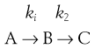
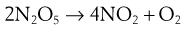
Molecularity is the number of molecules involved in forming the product. This follows from the balanced (stoichiometrical) equation describing the reaction. For example, in the following two-step reaction:

and

Order
This is the number of concentration terms that determine the rate. In a unimolecular process a molecule will react if it has sufficiently high energy. The number of high-energy molecules depends on how many molecules are present, i.e. on their concentration in solution (or pressure in a gas). In a bimolecular process, two molecules must collide to react and the likelihood of collision depends on the concentrations of each species. The Law of Mass Action states that the rate depends on the product of concentrations of the reactants.
Thus in the first step of the example reaction:
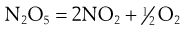
the rate of reaction = k1[N2O5]. Here k1 is the rate constant. The square brackets here, and throughout this chapter, mean ‘concentration of the entity within the brackets’. In this case there is only one concentration term and the reaction is known as first order.
In the second step:
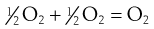
the rate of reaction = 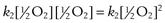 , where k2 is the reaction rate constant. Thus there are two concentration terms and the reaction is known as second order.
Each of these is discussed in more detail below.
First-order processes
The rate is determined by one concentration term. These are by far the most important processes in pharmaceutical science. Many drug decompositions during storage and the passage of drugs from one body compartment to another, e.g. lumen of the intestine into blood, follow first-order kinetics. The rate of reaction is most simply defined as the concentration change divided by the corresponding time change.
 (7.1)
(7.1)
The negative sign is used because concentration falls as time increases. This makes the rate constant, k, positive.
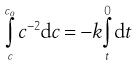
The differential equation above describes infinitely small changes. For real changes, these small changes are summed (integrated) usually from the start of the process (time = 0, concentration = co) to the concentration, c, remaining at any other time, t, as follows.
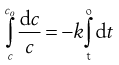 (7.2)
(7.2)
 (7.3)
(7.3)
 (7.4)
(7.4)
 (7.5)
(7.5)
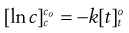
Thus a plot of ln c against t is a straight line with intercept ln c0 and gradient −k (Fig. 7.1).
The units of k are given by rearranging Equation 7.1, i.e.:
 (7.6)
(7.6)
Thus the rate constant has the dimensions of time−1 and typical units of s−1.
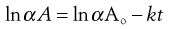
Note that because k contains no concentration term, it is not necessary to convert experimental data to concentration values in order to estimate it. Any convenient property of the system which is directly proportional to concentration can be used, such as UV absorbance, conductivity, pressure and radioactivity. For example, absorbance (A) is related to concentration, c, by Beer’s Law, i.e. c = αA, where α is a proportionality constant.
Substitution into Equation 7.5 gives:
 (7.7)
(7.7)
hence
 (7.8)
(7.8)
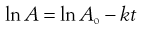
Thus the gradient is unchanged from Equation 7.7.
Box 7.1 Worked example
Consider the following example. A radio-labelled cardiac stimulant is administered by intravenous injection. Blood samples have the following radioactivity counts per second (cps).
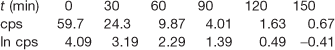
From Figure 7.1, it can be seen that the rate constant for absorption from the blood is 0.03 min−1.
Pseudo first-order processes
Consider the hydrolysis of ethyl acetate:

Strictly, the reaction is second order and the rate of reaction is expressed as follows. Again the square brackets used here and elsewhere in this chapter imply ‘concentration of’.
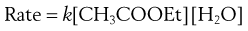
However, in a dilute aqueous solution of ethyl acetate, [H2O] is very large compared to [CH3COOEt] and hardly alters during the course of the reaction. [H2O] can be taken as a constant and incorporated into the second-order rate constant, now k′, where k′ = k[H2O]:
Thus, the reaction is, in effect, first order with a rate constant k′. This applies to many drug decompositions by hydrolysis in aqueous solution.
Second-order processes
The rate depends on the product of two concentration terms. In the simplest case they refer to the same species. For example:

Here the reaction is not simply a matter of a HI molecule falling apart, but relies on the collision of two HI molecules. The rate of reaction for this example is given from the Law of Mass Action by:
For a second-order process:
 (7.9)
(7.9)
 (7.10)
 (7.11)
 (7.12)
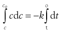
Thus the positive gradient of a plot of 1/c against t gives the rate constant, k (Fig. 7.2).
Units of k from Equation 7.9 are:
 (7.13)
i.e. conc−1 time−1 and typical units are L mole−1 s−1 or similar.
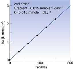
Box 7.2 Worked example
Consider the following decomposition data.
From Figure 7.2, it can be seen that the rate constant is 0.015 L mmole−1 day−1.
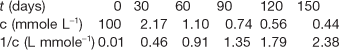
If the reaction is between two different species, A and B, it is unlikely that their starting concentrations will be equal. Let their initial concentrations be ao and bo (where ao > bo), falling to a and b at time t. Since equal numbers of molecules of A and B are lost in the decomposition, the rate can be defined as da/dt (or db/dt). Thus:
 (7.14)
Integration by partial fractions gives:
 (7.15)
Thus a plot of ln(a/b) against t is a straight line with gradient k(ao − bo).
Zero-order processes
In a zero-order reaction, the rate of process (decomposition, dissolution, drug release) is independent of the concentration of the reactants, i.e. the rate is constant. A constant rate of drug release from a dosage form is highly desirable. Zero-order kinetics often apply to processes occurring at phase boundaries, where the concentration at the surface remains constant either because reaction sites are saturated (enzyme kinetics, drug receptor interaction) or it is replenished constantly by diffusion of fresh material from within the bulk of one phase. This diffusion criterion applies to hydrolysis of drugs in suspensions and delivery from controlled-release dosage forms such as transdermal patches.
 (7.16)
 (7.17)
 (7.18)
 (7.19)
 (7.20)
Thus, a plot of c against t is a straight line with gradient −k (Fig. 7.3). Units of k from Equation 7.16 are concentration−1 time−1 with typical units of mole L−1 s−1 or similar.
Box 7.3 Worked example
The concentration of steroid remaining in a transdermal patch is as follows:

Note: strictly speaking, ‘amount’ is not the same as ‘concentration’ but in this case concentration can be considered to be µg patch−1.
From Figure 7.3, it can be seen that the rate constant is 0.12 µg h−1 (patch−1).
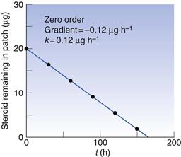
Fig. 7.3 Zero-order process, data plotted from Box 7.3.
Half-life, t1/2
This is the time taken for the concentration (of, say, a drug in solution or in the body) to reduce by a half.Rearrangement of the integrated equations for t (Eqns 7.5, 7.14 and 7.20) gives the relationships in the first line below and substituting c = co/2 at t1/2 gives those in the second line.
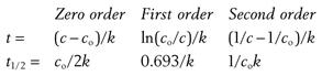
Note that for first-order reactions, the half-life, t1/2, is independent of concentration.
Summary of parameters
Table 7.1 summarizes the parameters for zero-order, first-order and second-order processes.
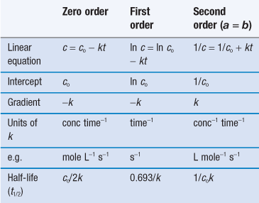
Determination of order and rate constant from experimental data
This can be achieved in two ways:
Box 7.4 Worked example
The following data apply to decomposition of a drug.

Data plotting method
The data of Box 7.4 are plotted in Figure 7.4. The plot of c against t (Fig. 7.4a) is obviously not linear so the reaction is not zero order. A plot of 1/c against time (Fig. 7.4b) is also not linear so the reaction is not second order.
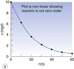
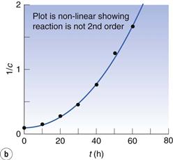
Fig. 7.4 (a) Plot of concentration against time. (b) Plot of 1/concentration against time. (c) Plot of ln (concentration) against time. Data plotted from Example 7.4.
However, a plot of ln c against t (Fig. 7.4c) is linear so the reaction is first order. From the graph, the gradient (i.e. −k) = −0.048 h−1 and the first-order rate constant = 0.048 h−1.
Half-life method
This involves the selection of a set of convenient ‘initial’ concentrations and then determining the times taken to fall to half these values.
Box 7.5 Worked example
The ‘co’ values are obtained by interpolation of the concentration versus time plot of the data in Box 7.4.
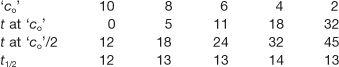
Within experimental error t1/2 seems independent of ‘co’, suggesting that the reaction is first order. To confirm this it is necessary to check whether t1/2 values correspond to zero- or second-order kinetics.
If the reaction was zero order, then co/2t1/2 would be a constant value (k). Similarly, for a second-order reaction, k = 1/cot1/2 would be constant. Calculating these gives:
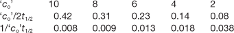
Thus, neither set of values is constant, confirming that the reaction is neither zero- or second-order.
The first-order rate constant is found from the mean t1/2 value of 13 h, i.e. k = 0.693/t1/2 = 0.053 h−1.
Complex reactions
The theories so far have assumed that a single reaction pathway is involved and that the product does not, in turn, affect the kinetics. Neither of these assumptions may be true and the overall order, being the result of several reactions, may not be zero, first or second order but have a fractional value.
There are three basic types of complex behaviour.
Parallel (side) reactions
Here reactants A form a mixture of products:
Usually only one of the products is desirable, the others are byproducts.
Series (consecutive) reactions
If k1 » k2 then a build-up of B occurs. The second (slower) step is then the ‘rate-determining’ step of the reaction, and the overall order is approximately that of the rate-determining step. Thus the reaction:
is composed of two consecutive reactions as discussed previously:


The overall reaction is first order, defined by the slower first step.
Reversible reactions
Here the product can reform into the reactants:
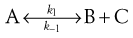
Here there are two reactions occurring simultaneously:
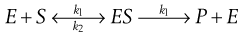
Michaelis–Menten equation
These three basic reaction types can be combined in different ways. One important combination describes processes that occur at interfaces. These appear repeatedly in the life sciences, e.g. enzyme–substrate, transmitter–receptor and drug–receptor binding. The kinetics are described by the Michaelis–Menten equation. This assumes that the enzyme, E, and substrate, S, form an unstable complex, ES, which can either reform S or form a new product, P.
 (7.21)
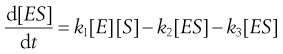
The overall reaction rate is the rate at which P is formed. This is first order depending on [ES], i.e. the concentration of ES. Thus dP/dt = k3[ES] (note that there is no negative sign because P increases as t increases).
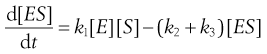
Unfortunately, we normally have no way of measuring [ES]. However, the rate at which [ES] changes is the rate at which it forms from E and S, (k1[E][S]), minus the rates at which it decomposes to reform E and S, (k2[ES]), or to form P, (k3[ES]). Thus:
 (7.22)
 (7.23)
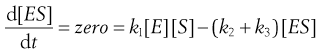
In practice [ES] is small as the complex decomposes rapidly. Changes in [ES] soon become negligible compared to other concentration changes in the system. Then [ES] is almost a constant, i.e. d[ES]/dt = zero, and the system is said to be at a ‘steady state’.
Thus at the steady state:
 (7.24)
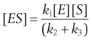
and rearrangement gives:
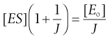
 (7.25)
Writing (k2 + k3)/k1 as K gives:
 (7.26)
 (7.27)
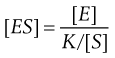
To proceed further, we need to know [ES], i.e. the concentration of the unstable intermediate. In practice we only know the total concentration of enzyme that we put into the mixture, [Eo]. Since this now exists in free and complexed forms then:
 (7.28)
Substituting [E] = [Eo] − [ES] in Equation 7.27 and then writing J = K/[S] gives:
 (7.29)
 (7.30)
 (7.31)
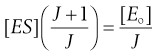 (7.32)
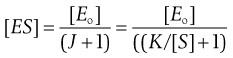 (7.33)
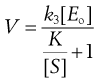
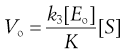
The overall rate of reaction, V, is given by the Michaelis–Menten equation:
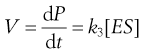 (7.34)
 (7.35)
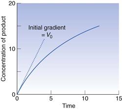
Thus the rate, V, is not constant but declines from its initial value, Vo, as [S] falls, i.e. as the substrate is used up. Vo is found from the initial gradient of the plot of [P] against t (Fig. 7.5).
If these Vo values are found for a range of substrate concentrations [S], and the enzyme concentration [Eo] is maintained constant, the familiar plateau curve results (Fig. 7.6). The plateau shape arises from the mathematical properties of the Michaelis–Menten equation.
 (7.36)
 (7.37)
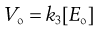
k3 and [Eo] are constants so this process is zero order. k3[Eo] is the maximum rate, Vmax, for a given enzyme concentration.
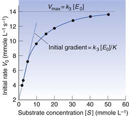
Viewed simply, the enzyme reactive sites are saturated by substrate molecules. This plateau curve is very common and often signifies a process occurring at a saturatable interphase, a heterogeneous process.
Equation 7.35 is often inverted to give a linear relationship between 1/V and 1/[S].
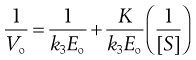 (7.38)
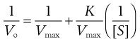 (7.39)
Vmax, K and k3 are found from the gradient and intercept of this Lineweaver–Burke plot (Fig. 7.7). Workers in the field of enzyme inhibition or drug–receptor interaction often estimate K from the intercept on the abscissa (x-axis) of the plot. This is the value of 1/[S] where 1/Vo = zero. Substitution into Equation 7.11 gives:
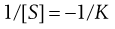 (7.40)
Thus from Figure 7.7, it can be seen that Vmax = 15.1 mmole L−1s−1 and K = 5.7. The way in which these parameters are altered by inhibitors enables us to say whether the inhibition is reversible/irreversible and competitive/non-competitive. York (1992) provides further details.
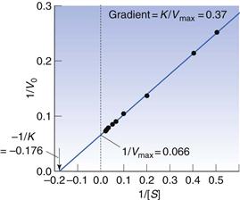
Fig. 7.7 Lineweaver–Burke plot of data in Figure 7.6.
Effect of temperature on reaction rate
Generally, increasing temperature increases the rate of reaction, and an often quoted rough guide is that a 10 °C rise doubles the rate constant. Better descriptions are given by the Arrhenius theory and the more rigorous transition state theory (see, for example, Martin 1993).
Arrhenius theory
This can be developed from simple basic ideas and leads to an equation that is formally identical with the transition state theory.
Consider the simple bimolecular reaction:
The original proposition was that if two molecules collided they would react. The collision number, Z, can be calculated from the kinetic theory of gases, and it was found that the number of molecules reacting per second, µ, was much smaller than Z. The theory was modified to propose that the colliding molecules must have sufficient energy to form an unstable intermediate, which breaks down to form the product.
The fraction of molecules with at least this activation energy, E, was calculated by Boltzmann as e−E/RT so that:
 (7.41)
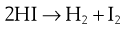
This equation adequately describes simple reactions like the decomposition of HI, but for even slightly more complex reactions such as:
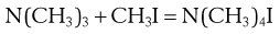
µ is thousands of times smaller than Ze−E/RT. This is because the nitrogen atom is shielded by a mass of C and H atoms, so that only very few collisions occur between the nitrogen and the carbon of the approaching CH3I. Thus an orientation factor, P, often with a very small value, must also be included.
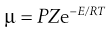 (7.42)
The rate constant k is proportional to µ. So, writing k as αµ (where α is the proportionality constant) gives:
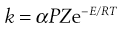 (7.43)
Over a small temperature range, the change in Z with T is negligible compared to that in the e−E/RT term, so that αPZ is a constant, A. A is called the ‘frequency factor’ since it is related to the frequency of correctly aligned collisions.
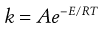 (7.44)
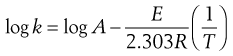
This is the Arrhenius equation, which may also be written as:
 (7.45)
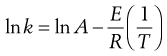
or in log10 form:
 (7.46)
so that a plot of ln k (or log k) against (1/T) is a straight line, enabling calculation of E and A from the gradient and intercept. (Remember that T must be in K, not °C.) The same equation holds for zero- and first-order reactions. Here the molecule will react if it has energy ≥ E.
The collision and orientation factors are inapplicable and A is now the proportionality constant α. However, it is still termed the frequency factor.
Box 7.6 Worked example
From the following data, estimate the rate constant at 25 °C.
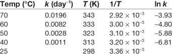
A plot of ln k against 1/T is a good straight line (Fig. 7.8).
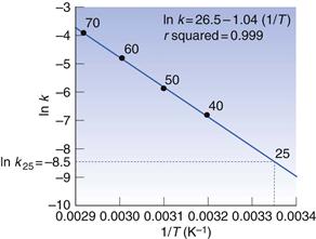
Reading ln k off the graph at 1/T = 3.36 × 10⁻³ (corresponding to 25 °C) is −8.5, giving k25 = 2.03 × 10⁻⁴ day−1.
Regression analysis (see, for example, Bolton 1984) gives the equation for the best straight line as ln k = 26.4 − 10408 1/T; correlation coefficient, r, of 0.999. Hence k25 = 1.98 × 10⁻⁴ day−1.
The 95% confidence interval is (1.35–2.95) × 10−4 day−1, showing that even good-quality experimental data yield disappointingly imprecise results on extrapolation.
The decomposition is first order and so obeys the equation:
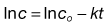 (7.47)
At the shelf-life, i.e. with a limit of 90% of stated active remaining, t10%, c = 0.9co, thus:
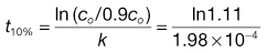
Thus, t10% = 527 days (95% confidence interval = 354–773 days).
References
1. Bolton S. Pharmaceutical Statistics. New York: Marcel Dekker; 1984.
2. Martin A. Physical Pharmacy. 4th edn Philadelphia: Lea and Febiger; 1993.
3. York JL. Enzymes: classification, kinetics and control. In: Devlin TM, ed. Textbook of Biochemistry. 3rd edn New York: John Wiley; 1992.
Bibliography
1. Saunders L, Fleming R. Mathematics and Statistics for Use in the Biological and Pharmaceutical Sciences. 2nd edn London: Pharmaceutical Press; 1971.
2. Singh UK, Orella CJ. Reaction kinetics and characterization. In In: am Ende DJ, ed. Chemical Engineering in the Pharmaceutical Industry: R&D to Manufacture. New Jersey, USA: John Wiley & Sons; 2010; (in conjunction with AIChE).
[/level-membership-for-basic-science-category][not-level-membership-for-basic-science-category]
Kinetics
W. John Pugh
Chapter contents
Homogeneous and heterogeneous reactions
Determination of order and rate constant from experimental data
Series (consecutive) reactions
Key points
• Kinetics is the study of the rate at which processes occur.
• Kinetic studies are useful in providing information that:
• gives an insight into the mechanisms of the changes involved and
• allows prediction of the degree of change that will occur after a given time has elapsed.
• The rate of a first-order process is determined by one concentration term.
• The rate of second-order processes depends on the product of two concentration terms.
• Better descriptions of the influence of temperature are given by the Arrhenius theory.
Introduction
Kinetics is the study of the rate at which processes occur. The changes may be chemical (e.g. decomposition of a drug, radiochemical decay) or physical (e.g. transfer across a boundary such as the intestinal lining or the skin). Kinetic studies are useful in providing information that:
• gives an insight into the mechanisms of the changes involved and
• allows prediction of the degree of change that will occur after a given time has elapsed.
In general, the theories and laws of chemical kinetics are well founded and provide a sound basis for the application of such studies to pharmaceutical problems that involve chemical and physical reactions.
The kinetics of processes have importance in a large number of areas of product design, manufacture, storage and drug delivery. These include: dissolution processes (Chapter 2), microbiological growth and destruction (Part 3), biopharmaceutics, including drug absorption, distribution, metabolism and excretion (Part 4), preformulation (Chapter 23), the rate of drug release from dosage forms (Part 5), and the decomposition of medicinal compounds and products (Part 6).
Homogeneous and heterogeneous reactions
Homogeneous reactions occur in a single phase, i.e. true solutions or gases, and proceed uniformly throughout the whole of the system. Heterogeneous reactions involve more than one phase and are often confined to the phase boundary, their rates being dependent on the supply of fresh reactants to this boundary. Examples are decomposition of drugs in suspensions and enzyme-catalysed reactions.
Molecularity
Molecularity is the number of molecules involved in forming the product. This follows from the balanced (stoichiometrical) equation describing the reaction. For example, in the following two-step reaction:
and
Order
This is the number of concentration terms that determine the rate. In a unimolecular process a molecule will react if it has sufficiently high energy. The number of high-energy molecules depends on how many molecules are present, i.e. on their concentration in solution (or pressure in a gas). In a bimolecular process, two molecules must collide to react and the likelihood of collision depends on the concentrations of each species. The Law of Mass Action states that the rate depends on the product of concentrations of the reactants.
Thus in the first step of the example reaction:
the rate of reaction = k1[N2O5]. Here k1 is the rate constant. The square brackets here, and throughout this chapter, mean ‘concentration of the entity within the brackets’. In this case there is only one concentration term and the reaction is known as first order.
In the second step:
the rate of reaction = , where k2 is the reaction rate constant. Thus there are two concentration terms and the reaction is known as second order.
Each of these is discussed in more detail below.
First-order processes
The rate is determined by one concentration term. These are by far the most important processes in pharmaceutical science. Many drug decompositions during storage and the passage of drugs from one body compartment to another, e.g. lumen of the intestine into blood, follow first-order kinetics. The rate of reaction is most simply defined as the concentration change divided by the corresponding time change.
(7.1)
The negative sign is used because concentration falls as time increases. This makes the rate constant, k, positive.
The differential equation above describes infinitely small changes. For real changes, these small changes are summed (integrated) usually from the start of the process (time = 0, concentration = co) to the concentration, c, remaining at any other time, t, as follows.
(7.2)
(7.3)
(7.4)
(7.5)
Thus a plot of ln c against t is a straight line with intercept ln c0 and gradient −k (Fig. 7.1).
The units of k are given by rearranging Equation 7.1, i.e.:
(7.6)
Thus the rate constant has the dimensions of time−1 and typical units of s−1.
Note that because k contains no concentration term, it is not necessary to convert experimental data to concentration values in order to estimate it. Any convenient property of the system which is directly proportional to concentration can be used, such as UV absorbance, conductivity, pressure and radioactivity. For example, absorbance (A) is related to concentration, c, by Beer’s Law, i.e. c = αA, where α is a proportionality constant.
Substitution into Equation 7.5 gives:
(7.7)
hence
(7.8)
Thus the gradient is unchanged from Equation 7.7.
Box 7.1 Worked example
Consider the following example. A radio-labelled cardiac stimulant is administered by intravenous injection. Blood samples have the following radioactivity counts per second (cps).
From Figure 7.1, it can be seen that the rate constant for absorption from the blood is 0.03 min−1.
Pseudo first-order processes
Consider the hydrolysis of ethyl acetate:
Strictly, the reaction is second order and the rate of reaction is expressed as follows. Again the square brackets used here and elsewhere in this chapter imply ‘concentration of’.
However, in a dilute aqueous solution of ethyl acetate, [H2O] is very large compared to [CH3COOEt] and hardly alters during the course of the reaction. [H2O] can be taken as a constant and incorporated into the second-order rate constant, now k′, where k′ = k[H2O]:
Thus, the reaction is, in effect, first order with a rate constant k′. This applies to many drug decompositions by hydrolysis in aqueous solution.
Second-order processes
The rate depends on the product of two concentration terms. In the simplest case they refer to the same species. For example:
Here the reaction is not simply a matter of a HI molecule falling apart, but relies on the collision of two HI molecules. The rate of reaction for this example is given from the Law of Mass Action by:
[/not-level-membership-for-basic-science-category]
