Image Processing
History of retinal imaging
The optical properties of the eye that allow image formation prevent direct inspection of the retina. Though existence of the red reflex has been known for centuries, special techniques are needed to obtain a focused image of the retina. The first attempt to image the retina, in a cat, was completed by the French physician Jean Mery, who showed that if a live cat is immersed in water, its retinal vessels are visible from the outside.1 The impracticality of such an approach for humans led to the invention of the principles of the ophthalmoscope in 1823 by Czech scientist Jan Evangelista  (frequently spelled Purkinje) and its reinvention in 1845 by Charles Babbage.2,3 Finally, the ophthalmoscope was reinvented yet again and reported by von Helmholtz in 1851.4 Thus, inspection and evaluation of the retina became routine for ophthalmologists, and the first images of the retina (Fig. 6.1) were published by the Dutch ophthalmologist van Trigt in 1853.5 The first useful photographic images of the retina, showing blood vessels, were obtained in 1891 by the German ophthalmologist Gerloff.6 In 1910, Gullstrand developed the fundus camera, a concept still used to image the retina today7; he later received the Nobel Prize for this invention. Because of its safety and cost-effectiveness at documenting retinal abnormalities, fundus imaging has remained the primary method of retinal imaging.
Fig. 6.1 First known image of human retina, as drawn by van Trigt in 1853. (Reproduced from Trigt AC. Dissertatio ophthalmologica inauguralis de speculo oculi. Utrecht: Universiteit van Utrecht, 1853.)
In 1961, Novotny and Alvis published their findings on fluorescein angiographic imaging.8 In this imaging modality, a fundus camera with additional narrow-band filters is used to image a fluorescent dye injected into the bloodstream that binds to leukocytes. It remains widely used, because it allows an understanding of the functional state of the retinal circulation.
The initial approach to depict the three-dimensional (3D) shape of the retina was stereo fundus photography, as first described by Allen in 1964, where multiangle images of the retina are combined by the human observer into a 3D shape.9 Subsequently, confocal scanning laser ophthalmoscopy (SLO) was developed, using the confocal aperture to obtain multiple images of the retina at different confocal depths, yielding estimates of 3D shape. However, the optics of the eye limit the depth resolution of confocal imaging to approximately 100 µm, which is poor when compared with the typical 300–500 µm thickness of the whole retina.10
OCT, first described in 1987 as a method for time-of-flight measurement of the depth of mechanical structures,11,12 was later extended to a tissue-imaging technique. This method of determining the position of structures in tissue, described by Huang et al. in 1991,13 was termed OCT. In 1993 in vivo retinal OCT was accomplished for the first time.14 Today, OCT has become a prominent biomedical tissue-imaging technique, especially in the eye, because it is particularly suited to ophthalmic applications and other tissue imaging requiring micrometer resolution.
History of retinal image processing
Matsui et al. were the first to publish a method for retinal image analysis, primarily focused on vessel segmentation.15 Their approach was based on mathematical morphology and they used digitized slides of fluorescein angiograms of the retina. In the following years, there were several attempts to segment other anatomical structures in the normal eye, all based on digitized slides. The first method to detect and segment abnormal structures was reported in 1984, when Baudoin et al. described an image analysis method for detecting microaneurysms, a characteristic lesion of diabetic retinopathy (DR).16 Their approach was also based on digitized angiographic images. They detected microaneurysms using a “top-hat” transform, a step-type digital image filter.17 This method employs a mathematical morphology technique that eliminates the vasculature from a fundus image yet leaves possible microaneurysm candidates untouched. The field dramatically changed in the 1990s with the development of digital retinal imaging and the expansion of digital filter-based image analysis techniques. These developments resulted in an exponential rise in the number of publications, which continues today.
Current status of retinal imaging
Retinal imaging has developed rapidly during the last 160 years and is a now a mainstay of the clinical care and management of patients with retinal as well as systemic diseases. Fundus photography is widely used for population-based, large-scale detection of DR, glaucoma, and age-related macular degeneration. OCT and fluorescein angiography are widely used in the daily management of patients in a retina clinic setting. OCT has also become an increasingly helpful adjunct in preoperative planning and postoperative evaluation of vitreoretinal surgical patients.18 The overview below is partially based on an earlier review paper.19
Fundus imaging
1. fundus photography (including so-called red-free photography): image intensities represent the amount of reflected light of a specific waveband
2. color fundus photography: image intensities represent the amount of reflected red (R), green (G), and blue (B) wavebands, as determined by the spectral sensitivity of the sensor
3. stereo fundus photography: image intensities represent the amount of reflected light from two or more different view angles for depth resolution
4. SLO: image intensities represent the amount of reflected single-wavelength laser light obtained in a time sequence
5. adaptive optics SLO: image intensities represent the amount of reflected laser light optically corrected by modeling the aberrations in its wavefront
6. fluorescein angiography and indocyanine angiography: image intensities represent the amounts of emitted photons from the fluorescein or indocyanine green fluorophore that was injected into the subject’s circulation.
There are several technical challenges in fundus imaging. Since the retina is normally not illuminated internally, both external illumination projected into the eye as well as the retinal image projected out of the eye must traverse the pupillary plane. Thus the size of the pupil, usually between 2 and 8 mm in diameter, has been the primary technical challenge in fundus imaging.7 Fundus imaging is complicated by the fact that the illumination and imaging beams cannot overlap because such overlap results in corneal and lenticular reflections diminishing or eliminating image contrast. Consequently, separate paths are used in the pupillary plane, resulting in optical apertures on the order of only a few millimeters. Because the resulting imaging setup is technically challenging, fundus imaging historically involved relatively expensive equipment and highly trained ophthalmic photographers. Over the last 10 years or so, there have been several important developments that have made fundus imaging more accessible, resulting in less dependence on such experience and expertise. There has been a shift from film-based to digital image acquisition, and as a consequence the importance of picture archiving and communication systems (PACS) has substantially increased in clinical ophthalmology, also allowing integration with electronic medical records. Requirements for population-based early detection of retinal diseases using fundus imaging have provided the incentive for effective and user-friendly imaging equipment. Operation of fundus cameras by nonophthalmic photographers has become possible due to nonmydriatic imaging, digital imaging with near-infrared focusing, and standardized imaging protocols to increase reproducibility.
Optical coherence tomography imaging
OCT is a noninvasive optical medical diagnostic imaging modality which enables in vivo cross-sectional tomographic visualization of the internal microstructure in biological systems. OCT is analogous to ultrasound B-mode imaging, except that it measures the echo time delay and magnitude of light rather than sound, therefore achieving unprecedented image resolutions (1–10 µm).20 OCT is an interferometric technique, typically employing near-infrared light. The use of relatively long-wavelength light with a very wide-spectrum range allows OCT to penetrate into the scattering medium and achieve micrometer resolution.
The principle of OCT is based upon low-coherence interferometry, where the backscatter from more outer retinal tissues can be differentiated from that of more inner tissues, because it takes longer for the light to reach the sensor. Because the differences between the most superficial and the deepest layers in the retina are around 300–400 µm, the difference in time of arrival is very small and requires interferometry to measure.21
We see the importance of the choice of a good low-coherence source – with either an incoherent or fully coherent source, interferometry is impossible. Such light can be generated by using superluminescent diodes (superbright light-emitting diodes) or lasers with extremely short pulses, femtosecond lasers. The optical setup typically consists of a Michelson interferometer with a low-coherence, broad-bandwidth light source (Fig. 6.2). By scanning the mirror in the reference arm, as in time domain OCT, modulating the light source, as in swept source OCT, or decomposing the signal from a broadband source into spectral components, as in spectral domain OCT (SD-OCT), a reflectivity profile of the sample can be obtained, as measured by the interferogram. The reflectivity profile, called an A-scan, contains information about the spatial dimensions and location of structures within the retina. A cross-sectional tomograph (B-scan) may be achieved by laterally combining a series of these axial depth scans (A-scan). En face imaging (C-scan) at an acquired depth is possible depending on the imaging engine used.
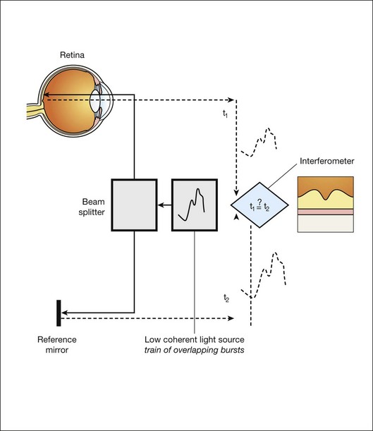
Fig. 6.2 Schematic diagram of the operation of an optical coherence tomography instrument, emphasizing splitting of the light in two arms, overlapping train of bursts “labeled” based on their autocorrelogram, and their interference after being reflected from retinal tissue as well as from the reference mirror (assuming the time delays of both paths are equal).
Time domain OCT
With time domain OCT, the reference mirror is moved mechanically to different positions, resulting in different flight time delays for the reference arm light. Because the speed at which the mirror can be moved is mechanically limited, only thousands of A-scans can be obtained per second. The envelope of the interferogram determines the intensity at each depth.13 The ability to image the retina two-dimensionally and three-dimensionally depends on the number of A-scans that can be acquired over time. Because of motion artifacts such as saccades, safety requirements limiting the amount of light that can be projected on to the retina, and patient comfort, 1–3 seconds per image or volume is essentially the limit of acceptance. Thus, the commercially available time domain OCT, which allowed collecting of up to 400 A-scans per second, has not yet been suitable for 3D imaging.
Frequency domain OCT
Spectral domain OCT
A broadband light source is used, broader than in time domain OCT, and the interferogram is decomposed spectrally using a diffraction grating and a complementary metal oxide semiconductor or charged couple device linear sensor. The Fourier transform is again applied to the spectral correlogram intensities to determine the depth of each scatter signal.22 With SD-OCT, tens of thousands of A-scans can be acquired each second, and thus true 3D imaging is routinely possible. Consequently, 3D OCT is now in wide clinical use, and has become the standard of care.
Swept source OCT
Instead of moving the reference arm, as with time domain OCT imaging, in swept source OCT the light source is rapidly modulated over its center wavelength, essentially attaching a second label to the light, its wavelength. A photo sensor is used to measure the correlogram for each center wavelength over time. A Fourier transform on the multiwavelength or spectral interferogram is performed to determine the depth of all tissue scatters at the imaged location.22 With swept source OCT, hundreds of thousands of A-scans can be obtained every second, with additional increase in scanning density when acquiring 3D image volumes.
Areas of active research in retinal imaging
Portable, cost-effective fundus imaging
For early detection and screening, the optimal place for positioning fundus cameras is at the point of care: primary care clinics, public venues (e.g., drug stores, shopping malls). Though the transition from film-based to digital fundus imaging has revolutionized the art of fundus imaging and made telemedicine applications feasible, the current cameras are still too bulky, expensive, and may be difficult to use for untrained staff in places lacking ophthalmic imaging expertise. Several groups are attempting to create more cost-effective and easier-to-use handheld fundus cameras, employing a variety of technical approaches.23,24
Functional imaging
For the patient as well as for the clinician, the outcome of disease management is mainly concerned with the resulting organ function, not its structure. In ophthalmology, current functional testing is mostly subjective and patient-dependent, such as assessing visual acuity and utilizing perimetry, which are all psychophysical metrics. Among more recently developed “objective” techniques, oxymetry is a hyperspectral imaging technique in which multispectral reflectance is used to estimate the concentration of oxygenated and deoxygenated hemoglobin in the retinal tissue.25 The principle allowing the detection of such differences is simple: deoxygenated hemoglobin reflects longer wavelengths better than does oxygenated hemoglobin. Nevertheless, measuring absolute oxygenation levels with reflected light is difficult because of the large variety in retinal reflection across individuals and the variability caused by the imaging process. The retinal reflectance can be modeled by a system of equations, and this system is typically underconstrained if this variability is not accounted for adequately. Increasingly sophisticated reflectance models have been developed to correct for the underlying variability, with some reported success.26 Near-infrared fundus reflectance in response to visual stimuli is another way to determine the retinal function in vivo and has been successful in cats. Initial progress has also been demonstrated in humans.27
Adaptive optics
The optical properties of the normal eye result in a point spread function width approximately the size of a photoreceptor. It is therefore impossible to image individual cells or cell structure using standard fundus cameras because of aberrations in the human optical system. Adaptive optics uses mechanically activated mirrors to correct the wavefront aberrations of the light reflected from the retina, and thus has allowed individual photoreceptors to be imaged in vivo.28 Imaging other cells, especially the clinically highly important ganglion cells, has thus far been unsuccessful in humans.
Longer-wavelength OCT imaging
3D OCT imaging is now the clinical standard of care for several eye diseases. The wavelengths around 840 µm used in currently available devices are optimized for imaging of the retina. Deeper structures, such as the choroidal vessels, which are important for AMD and other choroidal diseases, and the lamina cribrosa, relevant for glaucomatous damage, are not as well depicted. Because longer wavelengths penetrate deeper into the tissue, a major research effort has been undertaken to develop low-coherence swept source lasers with center wavelengths of 1000–1300 µm. Prototypes of these devices are already able to resolve detail in the choroid and lamina cribrosa.29
Clinical applications of retinal imaging
The most obvious example of a retinal screening application is retinal disease detection, in which the patient’s retinas are imaged in a remote telemedicine approach. This scenario typically utilizes easy-to-use, relatively low-cost fundus cameras, automated analyses of the images, and focused reporting of the results. This screening application has spread rapidly over the last few years, and, with the exception of the automated analysis functionality, is one of the most successful examples of telemedicine.30 While screening programs exist for detection of glaucoma, age-related macular degeneration, and retinopathy of prematurity, the most important screening application focuses on early detection of DR.
Early detection of diabetic retinopathy
Early detection of DR via population screening associated with timely treatment has been shown to prevent visual loss and blindness in patients with retinal complications of diabetes.31,32 Almost 50% of people with diabetes in the USA currently do not undergo any form of regular documented dilated eye exam, in spite of guidelines published by the American Diabetes Association, the American Academy of Ophthalmology, and the American Optometric Association.33 In the UK, a smaller proportion or approximately 20% of diabetics are not regularly evaluated, as a result of an aggressive effort to increase screening for people with diabetes. Blindness and visual loss can be prevented through early detection and timely management. There is widespread consensus that regular early detection of DR via screening is necessary and cost-effective in patients with diabetes.34–37 Remote digital imaging and ophthalmologist expert reading have been shown to be comparable or superior to an office visit for assessing DR and have been suggested as an approach to make the dilated eye exam available to unserved and underserved populations that do not receive regular exams by eye care providers.38,39 If all of these underserved populations were to be provided with digital imaging, the annual number of retinal images requiring evaluation would exceed 32 million in the USA alone (approximately 40% of people with diabetes with at least two photographs per eye).39,40 In the next decade, projections for the USA are that the average age will increase, the number of people with diabetes in each age category will increase, and there will be an undersupply of qualified eye care providers, at least in the near term. Several European countries have successfully instigated in their healthcare systems early detection programs for DR using digital photography with reading of the images by human experts. In the UK, 1.7 million people with diabetes were screened for DR in 2007–2008. In the Netherlands, over 30 000 people with diabetes were screened since 2001 in the same period, through an early-detection project called EyeCheck.41 The US Department of Veterans Affairs has deployed a successful photo screening program through which more than 120 000 veterans were screened in 2008. While the remote imaging followed by human expert diagnosis approach was shown to be successful for a limited number of participants, the current challenge is to make the early detection more accessible by reducing the cost and staffing levels required, while maintaining or improving DR detection performance. This challenge can be met by utilizing computer-assisted or fully automated methods for detection of DR in retinal images.42–44
Early detection of systemic disease from fundus photography
In addition to detecting DR and age-related macular degeneration, it also deserves mention that fundus photography allows certain cardiovascular risk factors to be determined. Such metrics are primarily based on measurement of retinal vessel properties, such as the arterial to venous diameter ratio, and indicate the risk for stroke, hypertension, or myocardial infarct.45,46
Image-guided therapy for retinal diseases with 3D OCT
Another highly relevant example of a disease that will benefit from image-guided therapy is exudative age-related macular degeneration. With the advent of the anti-vascular endothelial growth factor (VEGF) agents ranibizumab and bevacizumab, it has become clear that outer retinal and subretinal fluid is the main indicator of a need for anti-VEGF retreatment.47–51 Several studies are under way to determine whether OCT-based quantification of fluid parameters and affected retinal tissue can help improve the management of patients with anti-VEGF agents.
Image analysis concepts for clinicians
Image analysis is a field that relies heavily on mathematics and physics. The goal of this section is to explain the major clinically relevant concepts and challenges in image analysis, with no use of mathematics or equations. For a detailed explanation of the underlying mathematics, the reader is referred to the appropriate textbooks.52
The retinal image
Different strategies for storing ophthalmic images
• Slides and computer printouts stored in the paper chart or photo archive
• Slides and paper printouts scanned and stored in a PACS
• Clinically relevant views stored in a PACS
• All raw data and clinically relevant views stored in a PACS
• Standard for storage and communication of ophthalmology images.
Digital exchange of retinal images and DICOM
DICOM stands for Digital Imaging and Communications in Medicine and is an organization founded in 1983 to create a standard method for the transmission of medical images and their associated information across all fields of medicine. For ophthalmology, Working Group 9 (WG-9) of DICOM is a formal part of the American Academy of Ophthalmology. Until recently, the work of WG-9 has focused on creating standards for fundus, anterior-segment, and external ophthalmic photography, resulting in DICOM Supplement 91 Ophthalmic Photography Image SOP Classes, and on OCT imaging in DICOM Supplement 110: Ophthalmic Tomography Image Storage SOP53,54 (http://medical.nema.org).
Retinal image analysis
Common image-processing steps
Preprocessing
There are many parallels between image preprocessing using computers and human retinal image processing in ganglion cells.19
Detection
There are many parallels between the features and the convolution process in digital image analysis, and the filters in the human visual cortex.55
Unsupervised and supervised image analysis
The design and development of a retinal image analysis system usually involves the combination of some of the steps as explained above, with specific sizes of features and specific operations used to map the input image into the desired interpretation output. The term “unsupervised” is used to indicate such systems. The term “supervised” is used when the algorithm is improved in stepwise fashion by testing whether additional steps or a choice of different parameters can improve performance. This procedure is also called training. The theoretical disadvantage of using a supervised system with a training set is that the provenance of the different settings may not be clear. However, because all retinal image analysis algorithms undergo some optimization of parameters, by the designer or programer, before clinical use, this is only a relative, not absolute, difference. Two distinct stages are required for a supervised learning/classification algorithm to function: a training stage, in which the algorithm “statistically learns” to classify correctly from known classifications, and a testing or classification stage in which the algorithm classifies previously unseen images. For proper assessment of supervised classification method functionality, training data and performance testing data sets must be completely separate.52
Pixel feature classification
Pixel feature classification is a machine learning technique that assigns one or more classes to the pixels in an image.55,57 Pixel classification uses multiple pixel features including numeric properties of a pixel and the surroundings of a pixel. Originally, pixel intensity was used as a single feature. More recently, n-dimensional multifeature vectors are utilized, including pixel contrast with the surrounding region and information regarding the pixel’s proximity to an edge. The image is transformed into an n-dimensional feature space and pixels are classified according to their position in space. The resulting hard (categorical) or soft (probabilistic) classification is then used either to assign labels to each pixel (for example “vessel” or “nonvessel” in the case of hard classification), or to construct class-specific likelihood maps (e.g., a vesselness map for soft classification). The number of potential features in the multifeature vector that can be associated with each pixel is essentially infinite. One or more subsets of this infinite set can be considered optimal for classifying the image according to some reference standard. Hundreds of features for a pixel can be calculated in the training stage to cast as wide a net as possible, with algorithmic feature selection steps used to determine the most distinguishing set of features. Extensions of this approach include different approaches to classifying groups of neighboring pixels subsequently by utilizing group properties in some manner, for example cluster feature classification, where the size, shape, and average intensity of the cluster may be used.
Measuring performance of image analysis algorithms
Sensitivity and specificity
The performance of a lesion detection system can be measured by its sensitivity, which is the number of true positives divided by the sum of the total number of (incorrectly missed) false negatives plus the number of (correctly identified) true positives.52 System specificity is determined as the number of true negatives divided by the sum of the total number of false positives (incorrectly identified as disease) and true negatives. Sensitivity and specificity assessment both require ground truth, which is represented by location-specific discrete values (0 or 1) of disease presence or absence for each subject in the evaluation set. The location-specific output of an algorithm can also be represented by a discrete number (0 or 1). However, the output of the assessment algorithm is often a continuous value determining the likelihood p of local disease presence, with an associated probability value between 0 and 1. Consequently, the algorithm can be made more specific or more sensitive by setting an operating threshold on this probability value, p.
Receiver operator characteristics
If an algorithm outputs a continuous value, as explained above, multiple sensitivity/specificity pairs for different operating thresholds can be calculated. These can be plotted in a graph, which yields a curve, the so-called receiver operator characteristics or ROC curve.52,56 The area under this ROC curve (AUC, represented by its value Az) is determined by setting a number of different thresholds for the likelihood p. Sensitivity and specificity pairs of the algorithm are then obtained at each of these thresholds. The ground truth is kept constant. The maximum AUC is 1, denoting a perfect diagnostic procedure, with some threshold at which both sensitivity and specificity are 1 (100%).
The reference standard or gold standard
Typically these performance measurements are made by comparing the output of the image analysis system to some standard, usually called the reference standard or gold standard. Because the performance of some image analysis systems, for example for detection of DR, is starting to exceed that of individual clinicians or groups of clinicians, creating the reference standard is an area of active research.42
Given that determining the true state of disease necessary to create the reference standard is so challenging, the following options have been developed and are in wide use42:
1. Using the modality under study. The images are read and adjudicated by multiple trained readers according to a standardized protocol. This is less biased and a better estimate than a single clinician, but has higher cost. This method is often used, but the true disease is not known this way.
2. Using a different modality. In the case of a microaneurysm, an angiogram would be a suitable modality. It requires expert interpretation, and preferably multiple experts. It is less biased towards the imaging modality and may therefore be a better estimate. Because of the added procedure it is less patient-friendly, and has higher cost associated with it.
3. Doing a biopsy. Often this may be ethically unacceptable. It also displaces the problem, because the biopsy would necessarily be interpreted by human expert(s), for example a pathologist, with intra- and interobserver variability. It is more unequivocal, but also more invasive and has higher cost.
4. Outcome-based. If the clinically relevant question is not so much whether a microaneurysm is present or absent, but instead whether the patient is at risk of going blind from proliferative disease, we can wait for that outcome to occur. However, the true state of disease at this moment would still not be known, only the true state at some time in the past. Clinical outcome is maximally unequivocal and minimally subjective.
5. True state of disease, which is an unknowable quantity, as explained above.
Clinical safety relevant performance measurement
Performance of a system that has been developed for screening should not be evaluated based solely on its sensitivity and specificity for detection of that disease. Such metrics do not accurately reflect the complete performance in a screening setup. Rare, irregular, or atypical lesions often do not occur frequently enough in standard data sets to affect sensitivity and specificity but can have dramatic health and safety implications. To maximize screening relevance, the system must therefore include a mechanism to detect rare, atypical, or irregular abnormalities, for example in DR detection algorithms.43 For proper performance assessment, the types of potential false negatives – lesions that can be expected or shown to be incorrectly missed by the automated system – must be determined. While detection of red lesions and bright lesions is widely covered in the literature, detection of rare or irregular lesions, such as hemorrhages, neovascularization, geographic atrophy, scars, and ocular neoplasms has received much less attention, despite the fact that they all can occur in combination with DR and other retinal diseases, as well as in isolation. For example, presence of such lesions in isolated forms and without any co-occurrence of small red lesions is rare in DR; thus missing these does not affect standard metrics of performance to a measurable degree.41 One suitable approach for detecting such lesions is to use a retinal atlas, where the image is routinely compared to a generic normal retina. After building a retinal atlas by registering the fundus images according to a disc, fovea, and a vessel-based coordinate system, image properties at each atlas location from a previously unseen image can be compared to the atlas-based image properties. Consequently, locations can be identified as abnormal if groups of pixels have values outside the normal atlas range.
Fundus image analysis
Detection of retinal vessels
Automated segmentation of retinal vessels has been highly successful in the detection of large and medium vessels57–59 (Fig. 6.3). Because retinal vessel diameter and especially the relative diameters of arteries and veins are known to signal the risk of systemic disease, including stroke, accurate determination of retinal vessel diameters, as well as the ability to differentiate veins from arteries, has become more important. Several semiautomated and automated approaches to determining vessel diameter have now been published.60–62 Other active areas of research include separation of arteries and veins, detection of small vessels with diameters of less than a pixel, and analysis of complete vessel trees using graphs.
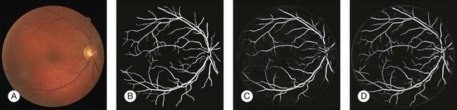
Fig. 6.3 Automated vessel analysis. (A) Fundus image; (B) retinal specialist annotation; (C) vesselness map from Staal algorithm (staal); (D) vesselness map from direct pixel classification. (Reproduced with permission from Niemeijer N, Staal JJ, van Ginneken B, et al. Comparative study of retinal vessel segmentation methods on a new publicly available database. In: Fitzpatrick JM, Sonka, editors. SPIE medical imaging, vol. 5370. SPIE, 2004, p. 648–56.)
Vessel detection approaches can be divided into region-based and edge-based approaches. Region-based segmentation methods label each pixel as either inside or outside a blood vessel. Niemeijer et al. proposed a pixel-based retinal vessel detection method using a gaussian derivative filter bank and k-nearest-neighbor classification.57,59 Staal et al.59 proposed a pixel feature-based method that additionally analyzed the vessels as elongated structures. Edge-based methods can be further classified into two categories: window-based methods and tracking-based methods. Window-based methods estimate a match at each pixel against the pixel’s surrounding window. The tracking approach exploits local image properties to trace the vessels from an initial point. A tracking approach can better maintain the connectivity of vessel structure. Lalonde et al.63 proposed a vessel-tracking method by following an edge line while monitoring the connectivity of its twin border on a vessel map computed using a Canny edge operator. Breaks in the connectivity will trigger the creation of seeds that serve as extra starting points for further tracking. Gang et al. proposed a retinal vessel detection using a second-order gaussian filter with adaptive filter width and adaptive threshold.64
Detection of fovea and optic disc
Location of the optic disc and fovea benefits retinal image analysis (Fig. 6.4). It is often necessary to mask out the normal anatomy before finding abnormal structures. For instance, the optic disc might be mistaken for a bright lesion if not detected. Secondly, the distribution of the abnormalities is not uniform on fundus photographs. Specific abnormalities occur more often in specific areas on the retina. Most optic disc detection methods are based on the fact that the optic disc is the convergence point of blood vessels and it is normally the brightest structure on a fundus image. Most fovea detection methods depend partially on the result of optic disc detection.
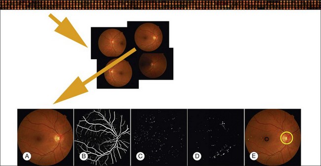
Fig. 6.4 Typical steps necessary for analysis of fundus images, in this case for early diabetic retinopathy. Top row: large sequence of image sets from multiple patients; second row: image set of four retinal images for a single patient; third row: (A) original image; (B) vesselness map; (C) automatically detected red lesions in white; (D) automatically detected bright lesions in white; and (E) detection of fovea (black) and optic disc (yellow) as well as automatically detected red lesions indicated in shades of green; bright lesions in shades of blue superimposed on original image.
Hoover et al. proposed a method for optic disc detection based on the combination of vessel structure and pixel brightness.65 If a strong vessel convergence point is found in the image, it is regarded as the optic disc. Otherwise the brightest region is detected. Foracchia et al. proposed an optic disc detection method based on vessel directions.66 A parabolic model of the main vascular arches is established and the model parameters are the directions associated with different locations on the parabolic model. The point with a minimum sum of square error is reported as the optic disc location. Lowell et al., by matching an optic disc model using the Pearson correlation, determined an initial optic disc location, and then traced the optic disc boundary using a deformable contour model.67
Most fovea detection methods use the fact that the fovea is a dark region in the image and that it normally lies in a fixed orientation and location relative to the optic disc and the main vascular arch. In a study by Fleming et al., approximate locations of the optic disc and fovea are obtained using the elliptical form of the main vascular arch.68 Then, the locations are refined based on the circular edge of the optic disc and the local darkness at the fovea. Li and Chutatape also proposed a method to select the brightest 1% pixels in a gray-level image.69 The pixels are clustered and principal component analysis based on a trained system is applied to extract a single point as the estimated location of the optic disc. A fovea candidate region is then selected based on the optic disc location and the main vascular arch shape. Within the candidate region, the centroid of the cluster with the lowest mean intensity and pixel number greater than one-sixth disc area is regarded as the foveal location. In a paper by Sinthanayothin et al., the optic disc was located as the area with the highest variation in intensity of adjacent pixels, while the fovea was extracted using intensity information and a relative distance to the optic disc.70 Tobin et al. proposed a method to detect the optic disc based on blood vessel features, such as density, average thickness, and orientation.71 Then the fovea location was determined based on the location of the optic disc and a geometry model of the main blood vessel. Niemeijer et al. proposed a method to localize automatically both the optic disc and fovea in 2006.72,73 For the optic disc detection, a set of features are extracted from the color fundus image. A k-nearest-neighbor classification is used to give a soft label to each pixel on the test image. The probability image is blurred and the pixel with the highest probability is detected as optic disc. Relative position information between the optic disc and the fovea is used to limit the search of fovea into a certain region. For each possible location of the optic disc, a possible location of the fovea is given. The possible locations for the fovea are stored in a separate image and the highest-probability location is detected as the fovea location.
Detection of retinal lesions
In this section we will primarily focus on detection of lesions in DR. DR has the longest history as a research subject in retinal image analysis. Figure 6.4 shows examples of a fundus photograph with the typical lesions automatically detected. After preprocessing, most approaches detect candidate lesions, after which a mathematical morphology template is utilized to segment and characterize the candidates (Fig. 6.5). This approach or a modification thereof is in use in many algorithms for detecting DR and age-related macular degeneration.74 Additional enhancements include the contributions of Spencer et al.75 and Frame et al.76 They added additional preprocessing steps, such as shade correction and matched filter postprocessing, to this basic framework to improve algorithm performance. Algorithms of this kind function by detecting candidate microaneurysms of various shapes, based on their response to specific image filters. A supervised classifier is typically developed to separate valid microaneurysms from spurious or false responses. However, these algorithms were originally developed to detect the high-contrast signatures of microaneurysms in fluorescein angiogram images. An important development was the addition of a more sophisticated filter, a modified version of the top-hat filter, so called because of its cross-section, to red-free fundus photographs rather than angiogram images, as was first described by Hipwell et al.77 They tested their algorithm on a large set of >3500 images and found a sensitivity/specificity operating point of 0.85/0.76. Once this filter-based approach had been established, development accelerated. The next step was broadening the candidate detection step, originally developed by Baudoin16 to detect candidate pixels, to a multifilter filter-bank approach.57,78 The responses of the filters are used to identify pixel candidates using a classification scheme. Mathematical morphology and additional classification steps are applied to these candidates to decide whether they indeed represent microaneurysms and hemorrhages (Fig. 6.6). A similar approach was also successful in detecting other types of DR lesions, including exudates and cotton-wool spots, as well as drusen in AMD.79
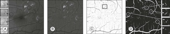
Fig. 6.5 Red lesion pixel feature classification. (A) Part of green color plane of a fundus image. Shown are pieces of vasculature and several red lesions. Circles mark the location of some of the red lesions in the image. (B) After subtracting median filtered version of the green plane, large background gradients are removed. (C) All pixels with a positive value are set to zero to eliminate bright lesions in the image. Note that exudates often partially occlude red lesions. Nonoccluded parts of red lesions show up clearly in this image. An example of this is marked with a rectangle. (D) Pixel classification result produced by contrast enhancement step. Nonoccluded parts of hemorrhages are visible together with the vasculature and a number of red lesions. (Reproduced with permission from Niemeijer M, van Ginneken B, Staal J, et al. Automatic detection of red lesions in digital color fundus photographs. IEEE Trans Med Imaging 2005;24:584–92.)
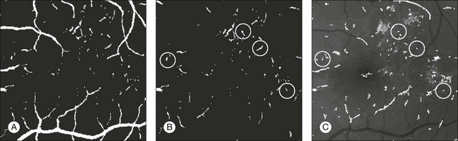
Fig. 6.6 Red lesion detection. (A) Thresholded probability map. (B) Remaining objects after connected component analysis and removal of large vasculature. (C) Shape and size of extracted objects in panel (B) do not correspond well with actual shape and size of objects in original image. Final region growing procedure is used to grow back actual objects in original image, which are shown here. In (B) and (C), the same red lesions as in Figure 6.6A are indicated with a circle. (Reproduced with permission from Niemeijer M, van Ginneken B, Staal J, et al. Automatic detection of red lesions in digital color fundus photographs. IEEE Trans MedImaging 2005;24:584–92.)
Initially, red lesions were detected in fluorescein angiograms because their contrast against the background is much higher than that of microaneurysms in color fundus photography images.75,76,80 Hemorrhages mask out fluorescence and present as dark spots in the angiograms. These methods employed a mathematical morphology technique that eliminated the vasculature from a fundus image but left possible microaneurysm candidates untouched, as first described in 1984.16 Later, this method was extended to high-resolution red-free fundus photographs by Hipwell et al.77 Instead of using morphology operations, a neural network was used, as demonstrated by Gardner et al.81 In their work, images are divided into 20 × 20 pixel grids and the grids are individually classified. Sinthanayothin et al. used a detection step to find blood-like regions and to segment both vessels and red lesions in a fundus image.82 A neural network was used to detect the vessels exclusively, and the remaining objects were labeled as microaneurysms. Niemeijer et al. presented a hybrid scheme that used a supervised pixel classification-based method to detect and segment the microaneurysm candidates in color fundus photographs.78 This method allowed for the detection of larger red lesions (i.e., hemorrhages) in addition to the microaneurysms using the same system. A large set of additional features, including color, was added to those that had been previously described.76,80 Using the features in a supervised classifier distinguished between real and spurious candidate lesions. These algorithms can usually distinguish between overlapping microaneurysms because they give multiple candidate responses.
Other recent algorithms only detect microaneurysms and forgo a phase of detecting normal retinal structures like the optic disc, fovea, and retinal vessels, which can act as confounders for abnormal lesions. Instead, the recent approaches find the microaneurysms directly using template matching in wavelet subbands.83 In this approach, the optimal adapted wavelet transform is found using a lifting scheme framework. By applying a threshold on the matching result of the wavelet template, the microaneurysms are labeled. This approach has meanwhile been extended explicitly to account for false negatives and false positives.42 Because it avoids detection of the normal structures, such algorithms can be very fast, on the order of less than a second per image.
Bright lesions, defined as lesions brighter than the retinal background, can be found in the presence of retinal and systemic disease. Some examples of such bright lesions of clinical interest include drusen, cotton-wool spots, and lipoprotein exudates. To complicate the analysis, flash artifacts can be present as false positives for bright lesions. If the lipoprotein exudates only appear in combination with red lesions, they would only be useful for grading DR. The exudates can, however, in some cases appear as isolated signs of DR in the absence of any other lesion. Several computer-based systems to detect exudates have been proposed (Fig. 6.7).74,79,81,82,84
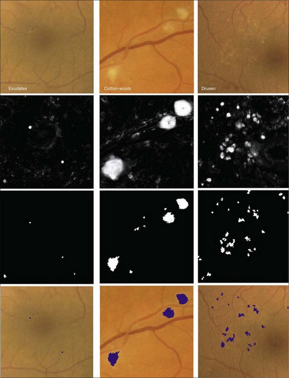
Fig. 6.7 Bright lesion detection algorithm steps performed to detect and differentiate “bright lesions.” From left to right: exudates, cotton-wool spots, and drusen. From top to bottom: relevant regions in the retinal color image (all at same scale); a posteriori probability maps after first classification step; pixel clusters labeled as probable bright lesions (potential lesions); bottom row shows final labeling of objects as true bright lesions, overlaid on original image. (Reproduced with permission from Niemeijer M, van Ginneken B, Russell SR, et al. Automated detection and differentiation of drusen, exudates, and cotton-wool spots in digital color fundus photographs for diabetic retinopathy diagnosis. Invest Ophthalmol Vis Sci 2007;48:2260–7.)
Because the different types of bright lesion have different diagnostic importance, algorithms should be capable not only of detecting bright lesions, but also of differentiating among the bright lesion types. One example algorithm capable of detection and differentiation of bright lesions was reported by Niemeijer et al. in 2007.79 This algorithm is based on an earlier red lesion algorithm presented by Hipwell et al. in 200077 and includes the following traditional steps, which are illustrated in Fig. 6.6:
1. lesion candidate cluster detection, where pixels are clustered into highly probable lesion regions
2. true bright lesion detection, where each candidate cluster is classified as a true lesion based on cluster features, including surface area, elongatedness, pixel intensity gradient, standard deviation of pixel values, pixel contrast, and local “vesselness” (as derived from a vessel segmentation map)
3. differentiation of lesions into drusen, exudates, and cotton-wool spots where a third classifier determines the likelihood for the true bright lesion to represent specific lesion types.
Vessel analysis
Vessel measures, such as the average width of arterioles and venules, the ratio of arteriolar to venular widths, and the branching ratio, have been established to be predictive of systemic diseases, especially hypertension, and also have potential value in degenerative retinal diseases such as retinitis pigmentosa. The methods in the section on detection of retinal vessels locate the vessels, but cannot determine vessel width. Additional techniques are needed to measure the vessel width accurately. Al-Diri et al. proposed an algorithm for segmentation and measurement of retinal blood vessels by growing a “ribbon of twins” active contour model. Their approach uses an extraction of segment profiles algorithm, which uses two pairs of contours to capture each vessel edge.85 The half-height full-width algorithm defines the width as the distance between the points on the intensity curve at which the function reaches half its maximum value to either side of the estimated center point.86–88 The Gregson algorithm fits a rectangle to the profile, setting the width so that the area under the rectangle is equal to the area under the profile.33 Xu et al. recently published a method based on graph search showing less variability than human experts (Fig. 6.8).89
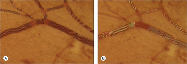
Fig. 6.8 Automated vessel width measurement. (A) Automated measurement of vessel width (black lines); (B) three human experts marking the widths of the vessel manually (in green, blue, and yellow).
A fully automated method from the Abramoff group to measure the arteriovenous ratio in disc center retinal images was recently published.90 This method detects the location of the optic disc, determines an appropriate region of interest, classifies vessels as arteries or veins, estimates vessel widths, and calculates the arteriovenous ratio. The system eliminates all vessels outside the arteriovenous ratio measurement region of interest. A skeletonization operation is then applied to the remaining vessels after which vessel crossings and bifurcation points are removed, leaving a set of vessel segments consisting of only vessel centerline pixels. Features are extracted from each centerline pixel in order to assign these a soft label indicating the likelihood that the pixel is part of a vein. As all centerline pixels in a connected vessel segment should be the same type, the median soft label is assigned to each centerline pixel in the segment. Next, artery vein pairs are matched using an iterative algorithm, and finally, the widths of the vessels are used to calculate the average arteriovenous ratio.
Retinal atlas
The retina has a relatively small number of key anatomic structures (landmarks) visible using planar fundus camera imaging. Additionally, the expected shape, size, and color variations across a population are expected to be high. While there have been a few reports on estimating retinal anatomic structure using a single retinal image,71 we are not aware of any published work demonstrating the construction of a statistical retinal atlas using data from a large number of subjects. The choice of atlas landmarks in retinal images may vary depending on the view of interest. Regardless, the atlas should represent most retinal image properties in a concise and intuitive way. Three landmarks can be used as the retinal atlas key features: the optic disc center, the fovea, and the main vessel arch defined as the location of the largest vein/artery pairs. The disc and fovea provide landmark points, while the arch is a more complicated two-part curved structure that can be represented by its central axis. The atlas coordinate system then defines an intrinsic, anatomically meaningful framework within which anatomic size, shape, color, and other characteristics can be objectively measured and compared. Choosing either the disc center or fovea alone to define the atlas coordinate system would allow each image from the population to be translated so pinpoint alignment can be achieved. Choosing both disc and fovea allows corrections for translation, scale, and rotational differences across the population. However, nonlinear shape variations across the population would not be considered – this can be accomplished when the vascular arch information is utilized. The end of the arches can be defined as the first major bifurcations of the arch branches. The arch shape and orientation vary from individual to individual and influence the structure of the remaining vessel network. Establishing an atlas coordinate system that incorporates the disc, fovea, and arches allows for translation, rotation, scaling, and nonlinear shape variations to be accommodated across a population.
An isotropic coordinate system is a system in which the size of each imaged element is the same in all three dimensions. This is desirable for a retinal atlas so images can refer to the atlas independent of spatial pixel location by a linear one-to-one mapping. The radial distortion correction (RADIC) model attempts to register images in a distortion-free coordinate system using a planar-to-spherical transformation, so the registered image is isotropic under a perfect registration, and places the registered image in an isotropic coordinate system (Fig. 6.9).91 An isotropic atlas makes it independent of spatial location to map correspondences between the atlas and test image. The intensities in overlapping area are determined by a distance-weighted blending scheme.92
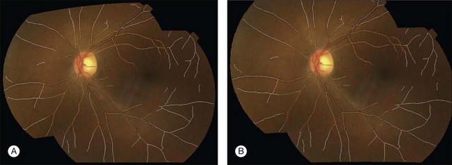
Fig. 6.9 Registration of fundus image pair using (A) quadratic model and (B) radial distortion correction model. Vessel center lines are overlaid for visual assessment of registration accuracy. This registration is performed to disc-centered and macula-centered images to provide an increased anatomic field of view. (Reproduced with permission from Lee S, Abramoff MD, Reinhardt JM. Retinal image mosaicing using the radial distortion correction model. In: Joseph MR, Josien PWP, eds. Proceedings of the SPIE. SPIE, 2008. p 691435.)
The atlas landmarks serve as the reference set so each color fundus image can be mapped to the coordinate system defined by the landmarks. As the last step of atlas generation, color fundus images are warped to the atlas coordinate system so that the arch of each image is aligned to the atlas vascular arch (Fig. 6.10).93 Rigid coordinate alignment is done for each fundus image to register the disc center and the fovea. The control points are determined by sampling points from equidistant locations in radial directions from the disc center. Usually, the sampling uses smoothed trace lines utilizing third-order polynomial curve fitting to eliminate locally high tortuosity of vascular tracings which may cause large geometric distortions (Fig. 6.11).
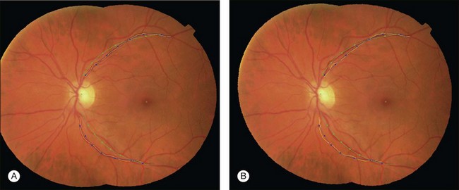
Fig. 6.10 Atlas coordinate mapping by thin plate spline (A) before and (B) after mapping. Naive main arch traces obtained by Dijkstra’s line detection algorithm are drawn as yellow lines that undergo polynomial curve fitting to result in blue lines. Atlas landmarks (disc center, fovea, and vascular arch) are drawn in green, and equidistant radial sampling points marked with dots. (Reproduced with permission from Abramoff MD, Garvin M, Sonka M. Retinal imaging and image analysis. IEEE Rev Biomed Eng 2010;3:169–208.)
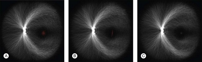
Fig. 6.11 Registration of anatomic structures according to increasing complexity of registration transform – 500 retinal vessel images are overlaid and marked with one foveal point landmark each (red spots). Rigid coordinate alignment by (A) translation, (B) translation and scale, and (C) translation, scale, and rotation. (Reproduced with permission from Abramoff MD, Garvin M, Sonka M. Retinal imaging and image analysis. IEEE Rev Biomed Eng 2010;3:169–208.)
A retinal atlas can be used as a reference to quantitatively assess the level of deviation from normality. An analyzed image can be compared with the retinal atlas directly in the atlas coordinate space. The normality can thus be defined in several ways depending on the application purpose – using local or global chromatic distribution, degree of vessel tortuosity, presence of pathological features, or presence of artifacts (Fig. 6.12). Other uses for a retinal atlas include image quality detection and disease severity assessment. Retinal atlases can also be employed in content-based image retrieval leading to abnormality detection in retinal images.94
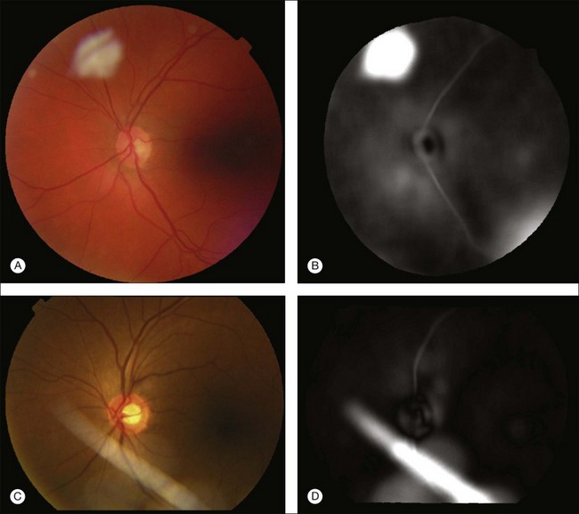
Fig. 6.12 Example application of employing retinal atlas to detect imaging artifacts. (A, C) Color fundus images with artifacts. (B, D) Euclidean distance maps in atlas space using atlas coordinate system. Note that distances are evaluated within atlas image. Consequently, field of view of distance map is not identical to that of fundus image. (Reproduced with permission from Abramoff MD, Garvin M, Sonka M. Retinal imaging and image analysis. IEEE Rev Biomed Eng 2010;3:169–208.)
Performance of DR detection algorithms
Several groups have studied the performance of detection algorithms in a real-world setting. The main goal of such a system is to decide whether the patient should be evaluated by a human expert or can return for routine follow-up, based solely on automated analysis of retinal images.43,44
DR detection algorithms appear to be mature and competitive algorithms and have now reached the human intrareader variability limit.41,42,95 Additional validation studies on larger, well-defined, but more diverse populations of patients with diabetes are urgently needed; anticipating cost-effective early detection of DR in millions of people with diabetes to triage those patients who need further care at a time when they have early rather than advanced DR. Validation trials are currently under way in the USA, UK, and the Netherlands.
To drive the development of progressively better fundus image analysis methods, research groups have established publicly available, annotated image databases in various fields. Fundus imaging examples are represented by the STARE,96 DRIVE,57 REVIEW,97 and MESSIDOR databases,98 with large numbers of annotated retinal fundus images, with expert annotations for vessel segmentation, vessel width measurements, and DR detection. Image analysis competitions such as the Retinopathy Online Challenge95 have also been initiated.
The Digital Retinal Images for Vessel Evaluation (DRIVE) database was established to enable comparative studies on segmentation of retinal blood vessels in retinal fundus images. It contains 40 fundus images from subjects with diabetes, both with and without retinopathy, as well as retinal vessel segmentations performed by two human observers. Starting in 2005, researchers have been invited to test their algorithms on this database and share their results with other researchers through the DRIVE website.89 At the same web location, results of various methods can be found and compared. Currently, retinal vessel segmentation research is primarily focusing on improved segmentation of small vessels, as well as on segmenting vessels in images with substantial abnormalities.
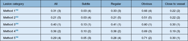
The DRIVE database was a great success, allowing comparisons of algorithms on a common data set. In retinal image analysis, it represented a substantial improvement over method evaluations on unknown data sets. However, different groups of researchers tend to use different metrics to compare the algorithm performance, making truly meaningful comparisons difficult or impossible. Additionally, even when using the same evaluation measures, implementation specifics of the performance metrics may influence final results. Consequently, until the advent of the Retinopathy Online Challenge competition in 2009, comparing the performance of retinal image analysis algorithms was difficult.95 This competition focused on detection of microaneurysms. Twenty-six groups participated in the competition, out of which six groups submitted their results on time. The results from each of the methods in this competition are summarized in Table 6.1.
Optical coherence tomography image analysis
SD-OCT technology has enabled true 3D volumetric scans of the retina to be acquired. Thus, the importance of developing advanced image analysis techniques to maximize the extraction of clinically relevant information is especially important. Nevertheless, the development of such advanced techniques can be challenging as OCT images are inherently noisy, thus often requiring the utilization of 3D contextual information (Fig. 6.13). Furthermore, the structure of the retina can drastically change during disease. Here, we review some of the important image analysis steps for processing OCT images. We start with the segmentation of retinal layers, one of the earliest, yet still extremely important, OCT image analysis areas. We then discuss techniques for flattening OCT images in order to correct scanning artifacts. Building upon the ability to extract layers, we discuss use of thickness information and of texture information. This is followed by the segmentation of retinal vessels, which currently has its technical basis in many of the techniques used for segmenting vessels in fundus photography, but is beginning to take advantage of the 3D information only available in SD-OCT. The use of both layer-based and texture-based properties to detect the locations of retinal lesions is then described. The ability to segment layers in the presence of lesions is described. This section is based on a review paper. 19
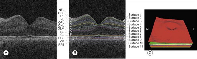
Fig. 6.13 Segmentation results of 11 retinal surfaces (10 layers). (A) X-Z image of optical coherence tomography volume. (B) Segmentation results: nerve fiber layer (NFL), ganglion cell layer (GCL), inner plexiform layer (IPL), inner nuclear layer (INL), outer plexiform layer (OPL), outer nuclear layer (ONL), outer limiting membrane (OLM), plus inner-segment layer (ISL), outer-segment layer (OSL), and retinal pigment epithelium complex (RPE). CL, Inner–outer segment interface complex surface; VM, Verhoeff’s membrane. (C) Three-dimensional rendering of segmented surfaces. N, nasal; T, temporal. (Reproduced with permission from Abramoff MD, Garvin M, Sonka M. Retinal imaging and image analysis. IEEE Rev Biomed Eng 2010;3:169–208.)
Retinal layer analysis from 3D OCT
The segmentation of retinal layers in OCT scans has been an important goal, because thickness changes in the layers are one indication of disease status. Previous-generation time domain scanning systems (such as the Stratus OCT by Carl Zeiss Meditec) offered the ability to segment and provide thickness measurements for a single layer of the retina. In particular, the retinal nerve fiber layer thickness measurements of peripapillary circular scans and total retinal thickness measurements were available and used clinically. It can be assumed that commercialized methods utilized an inherently 2D approach (i.e., if multiple 2D slices are available in a particular scanning sequence they are segmented independently). Indeed, most of the early approaches that have been reported in the literature99–104 for the segmentation of time domain scans are also 2D in nature.
While variations to each of the early 2D approaches exist for the segmentation of retinal boundaries, a typical 2D approach proceeds as follows: preprocess the image,99–101,103 perform a 1D peak detection (detection) on each A-scan of the processed image to find points of interest, and (in some methods) correct for possible discontinuities in the 1D border detection.99 Other 2D time domain approaches include the use of 2D dynamic programing by Baroni et al.105
Haeker et al.106–108 and Garvin et al.109 reported the first true 3D segmentation approach for the segmentation of retinal layers on OCT scans, taking advantage of 3D contextual information. Their approach was unique in that the layers were segmented simultaneously.110 For time domain macular scans, they segmented 6–7 surfaces (5–6 layers), obtaining an accuracy and reproducibility similar to that of retinal specialists. By extending the approach to SD-OCT volumes,111 utilization of 3D contextual information had more of an advantage (Fig. 6.14). By employing a multiscale approach, the processing time was subsequently decreased from hours to a few minutes while enabling segmenting additional layers.112 A similar approach for segmenting the intraretinal layers in optic nerve head-centered SD-OCT volumes was reported with an accuracy similar to that of the interobserver variability of two human experts.113 A preliminary layer thickness atlas was built from a small set of normal subjects. Thickness loss of the macular ganglion cell layer in people with diabetes without retinopathy was thus demonstrated, showing that diabetes also leads to retinal neuropathy.114,115
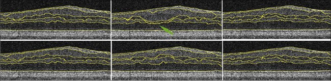
Fig. 6.14 An illustration of why using the complete three-dimensional (3D) contextual information in the intraretinal layer segmentation process is superior. (Top) Sequence of two-dimensional (2D) results on three adjacent slices within a spectral domain volume obtained using a slice-by-slice 2D graph-based approach. Note the “jump” in the segmentation result for third and fourth surfaces in middle slice. (Bottom) Sequence of 3D results on same three adjacent slices using same graph-based approach, but with the addition of 3D contextual information. 3D contextual information prevented third and fourth surface segmentation from failing.
OCT image flattening
SD-OCT volumes frequently demonstrate motion artifacts and other artifacts may also be present, such as the tilting due to an off-axis placement of the pupil. Approaches for reducing these artifacts include 1D and 2D methods that use cross-correlation of either A-scans100 or B-scans.116,117 In some cases, a complete flattening of the volume is desired based on a surface segmentation to ensure a consistent shape for segmentation and visualization. Flattening the volumes makes it possible to truncate the image substantially in the axial direction (z-direction), thereby reducing the memory and time requirements of an intraretinal layer segmentation approach. Flattening an image involves first segmenting the retinal pigment epithelial surface in a lower resolution, fitting a thin-plate spline to this surface, and then vertically realigning the columns of the volume to make this surface completely flat.111
Retinal layer thickness analysis
After flattening and segmentation, the properties of the macular tissues in each layer can be extracted and analyzed. In addition to layer thickness, textural properties can also be quantified, as explained in the next paragraph. Measuring the thickening of specific layers is crucial in the management of diabetic macular edema and other retinal disorders.118 Typically, it is useful to compare the obtained thickness values to a normative database or atlas, as is available in commercial machines for the total macular thickness and the retinal nerve fiber layer thickness. However, a normative atlas for all the layers in 3D currently only exists within individual research groups.119 Nevertheless, work has been done to demonstrate previously unknown changes in the ganglion cell layer in patients with diabetes.114,115
Retinal texture analysis
Texture, defined as measures of the spatial distribution of image intensities, can be used to characterize tissue properties and tissue differences. Textural properties may be important for assessing changes in the structural or tissue composition of layers that cannot be measured by changes in thickness alone. Texture can be determined in each of the identified layers three-dimensionally.83,120,121 3D formulations of texture descriptors were developed for pulmonary parenchymal analysis122 and have been directly employed for OCT texture analysis.123 The wavelet transform, a form of feature detection, has been used in OCT analysis for de-noising and de-speckling124–126 as well as for texture analysis.127 Early work on 3D wavelet analysis of OCT images was based on a computationally efficient yet flexible nonseparable lifting scheme in arbitrary dimensions.123,128
Texture characteristics can be computed for each segmented layer, several adjacent layers, or in layer combinations (Fig. 6.12).
Detection of retinal vessels from 3D OCT
Segmenting the retinal vasculature in 3D SD-OCT volumes129,130 allows OCT-to-fundus and OCT-to-OCT image registration. The absorption of light by the blood vessel walls causes vessel silhouettes to appear below the position of vessels, which thus causes the projected vessel positions to appear dark on either a full projection image of the entire volume130 or a projection image from a segmented layer for which the contrast between the vascular silhouettes and background is highest, as proposed by Niemeijer et al.129,131 In particular, this approach used the layer near the retinal pigment epithelium to create the projection image. Vessels were segmented using feature detection with gaussian filter-banks and a k-NN pixel classification approach. The performance of the automated method was evaluated for both optic nerve head-centered as well as macula-centered scans. The retinal vessels were successfully identified in a set of 16 3D OCT volumes (8 optic nerve head and 8 macula-centered), with high sensitivity and specificity as determined using ROC analysis, AUC = 0.96. Xu et al. reported an approach for segmenting the projected locations of the vasculature by utilizing pixel classification of A-scans.132 The features used in the pixel classification were based on a projection image of the entire volume in combination with features of individual A-scans. Both of these reported prior approaches focused on segmenting the vessels in the region outside the optic disc region because of difficulties in the segmentation inside this region. The neural canal opening shares similar features with vessels, thus causing false positives.133 Hu et al.127 proposed a modified 2D pixel classification algorithm to segment the blood vessels in SD-OCT volumes centered at the optic nerve head, with a special focus on better identifying vessels near the neural canal opening. Given an initial 2D segmentation of the projected vasculature, Lee et al. presented an approach for segmenting the 3D vasculature in the volumetric scans134 by utilizing a graph-theoretic approach (Fig. 6.15). One of the current limitations of that approach is the inability to resolve the depth information of crossing vessels properly.
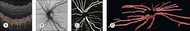
Fig. 6.15 Example of spectral three-dimensional (3D) optical coherence tomography (OCT) vessel segmentation. (A) Vessel silhouettes indicate position of vasculature. Also indicated in red are slice intersections of two surfaces that delineate the subvolume in which vessels are segmented (superficial retinal layers toward vitreous are at the bottom). (B) 2D projection image extracted from projected subvolume of spectral 3D OCT volume. (C) Automatic vessel segmentation. (D) 3D rendering of vessel around the optic nerve head. (Reproduced with permission from Lee K, Abràmoff M, Niemeijer MK, et al. 3D segmentation of retinal blood vessels in spectral-domain OCT volumes of the optic nerve head. Proc SPIE Med Imaging 2010;7626:76260 V.)
Detection of retinal lesions
Calculated texture and layer-based properties can be used to detect retinal lesions as a 2D footprint123 or in 3D. Out of many kinds of possible retinal lesions, symptomatic exudate-associated derangements (SEADs), a general term for fluid-related abnormalities in the retina, are of great interest in assessing the severity of choroidal neovascularization, diabetic macular edema, and other diseases. Detection of drusen, cotton-wool spots, areas of pigment epithelial atrophy, or pockets of fluid under epiretinal membranes may be attempted in a similar fashion.
The deviation of local retinal tissue from normal can be computed by determining the local deviations from the normal appearance at each location (x; y) in each layer and selecting the areas where the absolute deviation is greater than a predefined cutoff. More generally, in order to build an abnormality-specific detector, a classifier can be trained, the inputs of which may be the z-scores computed for relevant features. Comprehensive z-scores are appropriate since an abnormality may affect several layers in the neighborhood of a given location (x; y). The classifier-determined label associated with each column may be selected on relevant features by one of the many available cross-validation and/or feature selection methods,135–137 thus forming a SEADness or probabilistic abnormality map.
Fluid detection and segmentation
In choroidal neovascularization, diabetic macular edema, and other retinal diseases, intraretinal or subretinal fluid is reflective of disease status and changes in fluid are an indicator of disease progression or regression. With the availability of anti-VEGF therapy, assessment of the extent and morphology of fluid is expected to contribute to patient-specific therapy. While regions of fluid are inherently 3D, determining their 2D retinal footprint is highly relevant. Following the above-described analysis, fluid detection employs generalization of properties derived from expert-defined examples. Utilizing the differences between normal regional appearance of retinal layers as described by texture descriptors and other morphologic indices, a classifier can be trained to identify abnormal retinal appearance. The fluid detection starts with 3D OCT layer segmentation, resulting in 10 intraretinal layers, plus an additional artificial layer below the deepest intraretinal layer so that subretinal abnormalities can also be detected.123 Texture-based and morphologic descriptors are calculated regionally in rectangular subvolumes, the most discriminative descriptors are identified, and these descriptors are used for training a probabilistic classifier. The performance of a (set of) feature(s) is assessed by calculating the area under the ROC of the fluid classifier. Once the probabilistic classifier is trained, fluid-related probability is determined for each retinal location. In order to obtain a binary footprint for fluid in an image input to the system, the probabilities are thresholded and the footprint of the fluid region in this image is defined as the set of all pixels with a probability greater than a threshold. Useful 3D textural information can be extracted from SD-OCT scans and, together with an anatomical atlas of normal retinas, can be used for clinically important applications.
Fluid segmentation in 3D
Complete volumetric segmentation of fluid from 3D OCT is the subject of active research. A promising approach is based on identification of a seed point in the OCT data set that is “inside” and “outside” a fluid region. These points can be identified automatically using a 3D variant of the probabilistic classification approach outlined in the previous paragraphs. Once these two points are identified, an automated segmentation procedure that is based on regional graph-cut method138,139 may be employed to detect the fluid volumetric region. The cost function utilized in a preliminary study was designed to identify dark 3D regions with somewhat homogeneous appearance. The desired properties of the fluid region are automatically learned from the vicinity of the identified fluid region seed point. This adaptive behavior allows the same graph-cut segmentation method driven by the same cost function to segment fluid of different appearance reliably. Figure 6.16 gives an example of 3D fluid region segmentations obtained using this approach. Note that the figure depicts the same locations in the 3D data sets imaged several times during the course of anti-VEGF treatment. The surfaces of the segmented fluid regions are represented by a 3D mesh, which can be interactively edited to maximize fluid region segmentation accuracy in difficult or ambiguous cases.
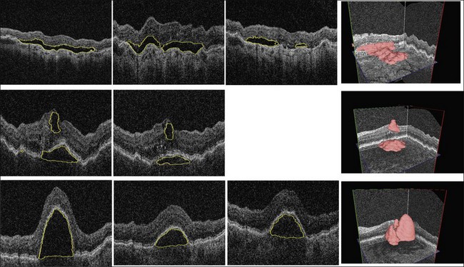
Fig. 6.16 Symptomatic exudate-associated derangement (SEAD) segmentation from three-dimensional optical coherence tomography and SEAD development over time. Top row: 0, 28, and 77 days after first imaging visit. Middle row: 0 and 42 days after first imaging visit. Bottom row: 0, 14, and 28 days after first imaging visit. Three-dimensional visualization in right column shows data from week 0. Each imaging session was associated with anti-vascular endothelial growth factor reinjection.
Multimodality retinal imaging
Multimodality imaging, defined as images from the same organ acquired using different techniques using different physical techniques, is becoming increasingly common in ophthalmology. For image information from multiple modalities to be usable in mutual context, images must be registered so that the independent information that was acquired by different methods can be concatenated and form a multimodality description vector. Thus, because of its importance in enabling multimodal analysis, retinal image registration reflects another active area of research. The several clinically used methods to image the retina were introduced above and include fundus photography, SLO, fluorescence imaging, and OCT. Additional retinal imaging techniques, such as hyperspectral imaging, oximetry, and adaptive optics SLO, will bring higher resolution and additional image information. To achieve a comprehensive description of retinal morphology and eventually function, diverse retinal images acquired by different or the same modalities at different time instants must be mutually registered to combine all available local information spatially. The following sections provide a brief overview of fundus photography and OCT registration approaches in both 2D and 3D; a more detailed review is available.19 Registration of retinal images from other existing and future imaging devices can be performed in a similar or generally identical manner.
Registration of fundus retinal photographs
Registration of fundus photographs taken either at different regions of the retina, or of the same area of the retina but at different times, is useful to expand the effective field of view of a retinal image, determine what part of the retina is being viewed, or aid in analyzing changes over time.140 We have previously discussed some other uses for fundus–fundus registration in regard to retinal atlases. To register 2D or planar fundus images, most existing registration approaches utilize identification and extraction of features derived from retinal vasculature segmented separately from the individual fundus images. The choice of a specific image registration algorithm to align retinal images into a montage depends on the image characteristics and the application. Images acquired with only a small overlap may be optimally aligned using feature-based registration approaches, while images acquired with larger overlaps may be satisfactorily aligned using intensity-based approaches. Examples of feature-based registration are global-to-local matching,141 hierarchical model refinement,142 and dual-bootstrap.143 Local intensity features144 are particularly useful when an insufficient number of vascular features are available. Following a step of vascular skeletonization, vascular branching points can be easily used as stable landmarks for determining image-to-image correspondence. As an example, the RADIC model145 parameters are estimated during an optimization step that uses Powell’s method146 and is driven by the vessel centerline distance. The approach presented by Lee et al. in 2010 reported registration accuracy of 1.72 pixels (25–30 µm, depending on resolution) when tested in 462 pairs of green channel fundus images.147 The registration accuracy was assessed as the vessel line error. The method only needed two correspondence points to be reliably identified and was therefore applicable even to cases when only a very small overlap between the retinal image pairs existed. Based on the identified vascular features, the general approach can be applied to any retinal imaging modality for which a 2D vessel segmentation is available. In registering poor-quality multimodal fundus image pairs, which may not have sufficient vessel-based features available, Chen et al. proposed the detection of corner points using a Harris detector followed by use of a partial intensity invariant feature descriptor.148 They reported obtaining 89.9% “acceptable” registrations (defined as registrations with a median error of 1.5 pixels and a maximum error of 10 pixels when compared with ground truth correspondences) when tested on 168 pairs of multimodal retinal images.
Registration of OCT with fundus retinal photographs
Registration of 2D fundus images with inherently 3D OCT images requires that the dimensionality of OCT be reduced to 2D via z-axis projection. Building on the ability to obtain vascular segmentation from 3D OCT projection images, the problem of fundus–OCT registration becomes virtually identical to that of fundus–fundus registration that was described in the previous section. Using the same general method, high-quality OCT–fundus registration can be achieved. Figure 6.17 presents the main steps of the registration process and shows the registration performance achieved.
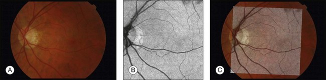
Fig. 6.17 Registration of fundus images to 2D optical coherence tomography (OCT) projection data. (A) Fundus camera image. (B) 2D projection (through depth dimension) of three-dimensional OCT data. (C) Registered and blended fundus OCT images via application of affine transformation model with three identified vascular landmarks.
Mutual registration of 3D OCT images
Temporal changes of retinal layers leading to assessment of disease progression or regression can be accessed from longitudinal OCT images. Comparison of morphology or function over time requires that the respective OCT image data sets be registered. Since OCT is a 3D imaging modality, such registration needs to be performed in 3D. For follow-up studies, image registration is a vital tool to enable more precise, quantitative comparison of disease status. Another important aspect of OCT–OCT registration is the ability to enlarge retinal coverage by registering OCT data resulting from imaging different portions of the retina. A fully 3D scale-invariant feature transform (SIFT)-based approach was introduced in 2009.149 The SIFT feature extractor locates minima and maxima in the difference of gaussian scale space to identify salient feature points. Using calculated histograms of local gradient directions around each found extremum in 3D, the matching points are found by comparing the distances between feature vectors. An application of this approach to rigid registration of peripapillary (ONH-centered) and macula-centered 3D OCT scans of the same patient for which the macular and peripapillary OCT scans had only a limited overlap has been reported.148 The work built on a number of analysis steps introduced earlier, including segmentation of the main retinal layers and 3D flattening of each of the two volumes to be registered. 3D SIFT feature points were subsequently determined.150,151 Using the customary terminology for image registration, when one of the registered images is called the “source” (say the macular image) and the other the “target” (say the peripapillary image), the feature point detection is performed in both source and target images. After feature point extraction, those which are in corresponding positions in both images are identified. In a typical pair of two OCT scans, about 70 matching pairs can be found with a high level of certainty. The primary deformations that need to be resolved are translation and limited rotation, so simple rigid or affine transform is appropriate to achieve the desired image registration. The transform parameters are estimated from the identified correspondence points. Niemeijer et al. demonstrated the functionality of such an approach to OCT–OCT registration of macular and peripapillary OCT scans.149 3D registration achieved 3D accuracy of 2.0 ± 3.3 voxels, assessed as an average voxel distance error in 1572 matched locations. Qualitative evaluation of performance demonstrated the utility of this approach to clinical-quality images. Temporal registration of longitudinally acquired OCT images from the same subjects can be obtained in an identical manner.
Future of retinal imaging and image analysis
Translation of research in imaging and image analysis into the clinic has been relatively rapid in the past, and can be expected to accelerate in the future. This is partially explained by the lower capital expenditure for ophthalmic imaging devices compared to radiologic imaging devices – the latter can often be 10–100 times more expensive – and also because retinal specialists manage patients directly and are directly involved in the ordering and interpreting of images, while radiologists typically do not directly manage patients. This subtle difference in the physician–patient relationship leads to a more direct coupling between imaging innovation and clinical impact that is so visible in retinal imaging and analysis. Given the above, it can be expected that translation of fundamental research findings in retinal imaging will remain rapid in the future. The need to computerize and automate image interpretation is correspondingly high. A global push toward cost-effective imaging and image analysis for wide-scale retinal and/or systemic disease detection in a population-screening setting will mandate continued efforts in perfecting automated image analysis.19
References
1. Zhang, X, Saaddine, JB, Chou, CF, et al. Prevalence of diabetic retinopathy in the United States, 2005–2008. JAMA. 2010;304:649–656.
2. Flick, CS. Centenary of Babbage’s ophthalmoscope. Optician. 1947;113:246.
3. Keeler, CR. 150 years since Babbage’s ophthalmoscope. Arch Ophthalmol. 1997;115:1456–1457.
4. von Helmholtz, H. Beschreibung eines Augens-Spiegels zur Untersuchung der Netzhaut im lebenden Auge. Berlin: Foerstner; 1851.
5. Trigt, AC. Dissertatio ophthalmologica inauguralis de speculo oculi. Utrecht: Universiteit van Utrecht; 1853.
6. Gerloff, O. Über die Photographie des Augenhintergrundes. Klin Monbl Augenheilkd. 1891;29:397ff.
7. Gullstrand, A. Neue methoden der reflexlosen. Ophthalmoskopie. Berichte Dtsch Ophthalmologische Gesellschaft. 1910:36.
8. Novotny, HR, Alvis, DL. A method of photographing fluorescence in circulating blood in the human retina. Circulation. 1961;24:82–86.
9. Allen, L. Ocular fundus photography: suggestions for achieving consistently good pictures and instructions for stereoscopic photography. Am J Ophthalmol. 1964;57:13–28.
10. Webb, RH, Hughes, GW. Scanning laser ophthalmoscope. IEEE Trans Biomed Eng. 1981;28:488–492.
11. Youngquist, RC, Carr, S, Davies, DE. Optical coherence-domain reflectometry: a new optical evaluation technique. Optics Lett. 1987;12:158–160.
12. Youngquist RC, Wentworth RH, Fesler KA. Selective interferometric sensing by the use of coherence synthesis. Optics Lett 1987;12:944–6.
13. Huang, D, Swanson, EA, Lin, CP, et al. Optical coherence tomography. Science. 1991;254:1178–1181.
14. Swanson, EA, Izatt, JA, Hee, MR, et al. In vivo retinal imaging by optical coherence tomography. Optics Lett. 1993;18:1864–1866.
15. Matsui, M, Tashiro, T, Matsumoto, K, et al. [A study on automatic and quantitative diagnosis of fundus photographs. I. Detection of contour line of retinal blood vessel images on color fundus photographs (author’s transl).]. Nippon Ganka Gakkai Zasshi. 1973;77:907–918.
16. Baudoin, CE, Lay, BJ, Klein, JC. Automatic detection of microaneurysms in diabetic fluorescein angiography. Rev Epidemiol Sante Publique. 1984;32:254–261.
17. Wild, S, Roglic, G, Green, A, et al. Global prevalence of diabetes: estimates for the year 2000 and projections for 2030. Diabetes Care. 2004;27:1047–1053.
18. Germain, N, Galusca, B, Deb-Joardar, N, et al. No loss of chance of diabetic retinopathy screening by endocrinologists with a digital fundus camera. Diabetes Care. 2011;34:580–585.
19. Abramoff, MD, Garvin, M, Sonka, M. Retinal imaging and image analysis. IEEE Rev Biomed Eng. 2010:169–208.
20. Fujimoto, JG. Optical coherence tomography for ultrahigh resolution in vivo imaging. Nat Biotechnol. 2003;21:1361–1367.
21. Fercher, AF, Mengedoht, K, Werner, W. Eye-length measurement by interferometry with partially coherent light. Optics Lett. 1988;13:186–188.
22. Choma, M, Sarunic, M, Yang, C, et al. Sensitivity advantage of swept source and Fourier domain optical coherence tomography. Optics Express. 2003;11:2183–2189.
23. Abramoff, MD, Kardon, RH, Vermeer, KA, et al. A portable, patient friendly scanning laser ophthalmoscope for diabetic retinopathy imaging: exudates and hemorrhages. Invest Ophthalm Vis Sci. 2007:48.
24. Hammer, DX, Ferguson, RD, Ustun, TE, et al. Line-scanning laser ophthalmoscope. J Biomed Opt. 2006;11:041126.
25. Suansilpong, A, Rawdaree, P. Accuracy of single-field nonmydriatic digital fundus image in screening for diabetic retinopathy. J Med Assoc Thai. 2008;91:1397–1403.
26. Delori, FC, Pflibsen, KP. Spectral reflectance of the human ocular fundus. Appl Opt. 1989;28:1061–1077.
27. Abramoff, MD, Kwon, YH, Ts’o, D, et al. Visual stimulus-induced changes in human near-infrared fundus reflectance. Invest Ophthalmol Vis Sci. 2006;47:715–721.
28. Whited, JD. Accuracy and reliability of teleophthalmology for diagnosing diabetic retinopathy and macular edema: a review of the literature. Diabetes Technol Ther. 2006;8:102–111.
29. Lin, DY, Blumenkranz, MS, Brothers, R. The role of digital fundus photography in diabetic retinopathy screening. Digital Diabetic Screening Group (DDSG). Diabetes Technol Ther. 1999;1:477–487.
30. Standards and Guidelines in Telehealth for Diabetic Retinopathy: American Telemedicine Association position statement. http://www.americantelemed.org/ICOT/drpositionpaper.paper.technical.htm.
31. Bresnick, GH, Mukamel, DB, Dickinson, JC, et al. A screening approach to the surveillance of patients with diabetes for the presence of vision-threatening retinopathy. Ophthalmology. 2000;107:19–24.
32. Kinyoun, JL, Martin, DC, Fujimoto, WY, et al. Ophthalmoscopy versus fundus photographs for detecting and grading diabetic retinopathy. Invest Ophthalmol Vis Sci. 1992;33:1888–1893.
33. Preferred Practice Pattern. Diabetic Retinopathy. www.aao.org/ppp.
34. Fong, DS, Aiello, L, Gardner, TW, et al. Diabetic retinopathy. Diabetes Care. 2003;26:226–229.
35. Fong, DS, Sharza, M, Chen, W, et al. Vision loss among diabetics in a group model Health Maintenance Organization (HMO). Am J Ophthalmol. 2002;133:236–241.
36. Wilson, C, Horton, M, Cavallerano, J, et al. Addition of primary care-based retinal imaging technology to an existing eye care professional referral program increased the rate of surveillance and treatment of diabetic retinopathy. Diabetes Care. 2005;28:318–322.
37. Klonoff, DC, Schwartz, DM. An economic analysis of interventions for diabetes. Diabetes Care. 2000;23:390–404.
38. Lin, DY, Blumenkranz, MS, Brothers, RJ, et al. The sensitivity and specificity of single-field nonmydriatic monochromatic digital fundus photography with remote image interpretation for diabetic retinopathy screening: a comparison with ophthalmoscopy and standardized mydriatic color photography. Am J Ophthalmol. 2002;134:204–213.
39. Williams, GA, Scott, IU, Haller, JA, et al. Single-field fundus photography for diabetic retinopathy screening: a report by the American Academy of Ophthalmology. Ophthalmology. 2004;111:1055–1062.
40. Lawrence, MG. The accuracy of digital-video retinal imaging to screen for diabetic retinopathy: an analysis of two digital-video retinal imaging systems using standard stereoscopic seven-field photography and dilated clinical examination as reference standards. Trans Am Ophthalmol Soc. 2004;102:321–340.
41. Abramoff, MD, Suttorp-Schulten, MS. Web-based screening for diabetic retinopathy in a primary care population: the EyeCheck project. Telemed J E Health. 2005;11:668–674.
42. Abramoff, MD, Reinhardt, JM, Russell, SR, et al. Automated early detection of diabetic retinopathy. Ophthalmology. 2010;117:1147–1154.
43. Abramoff, MD, Niemeijer, M, Suttorp-Schulten, MS, et al. Evaluation of a system for automatic detection of diabetic retinopathy from color fundus photographs in a large population of patients with diabetes. Diabetes Care. 2008;31:193–198.
44. Philip, S, Fleming, AD, Goatman, KA, et al. The efficacy of automated “disease/no disease” grading for diabetic retinopathy in a systematic screening programme. Br J Ophthalmol. 2007;91:1512–1517.
45. Cheung, N, Rogers, S, Couper, DJ, et al. Is diabetic retinopathy an independent risk factor for ischemic stroke? Stroke. 2007;38:398–401.
46. Photocoagulation treatment of proliferative diabetic retinopathy: the second report of diabetic retinopathy study findings. Ophthalmology. 1978;85:82–106.
47. Rosenfeld, PJ, Moshfeghi, AA, Puliafito, CA. Optical coherence tomography findings after an intravitreal injection of bevacizumab (Avastin) for neovascular age-related macular degeneration. Ophthalm Surg Lasers Imaging. 2005;36:331–335.
48. Heier, JS, Antoszyk, AN, Pavan, PR, et al. Ranibizumab for treatment of neovascular age-related macular degeneration: a phase I/II multicenter, controlled, multidose study. Ophthalmology. 2006;113:633.e1–633.e4.
49. Preliminary report on effects of photocoagulation therapy. The Diabetic Retinopathy Study Research Group. Am J Ophthalmol. 1976;81:383–396.
50. Grading diabetic retinopathy from stereoscopic color fundus photographs – an extension of the modified Airlie House classification. ETDRS report number 10. Early Treatment Diabetic Retinopathy Study Research Group. Ophthalmology. 1991;98:786–806.
51. Harvey, JN, Craney, L, Nagendran, S, et al. Towards comprehensive population-based screening for diabetic retinopathy: operation of the North Wales diabetic retinopathy screening programme using a central patient register and various screening methods. J Med Screen. 2006;13:87–92.
52. Sonka, M, Fitzpatrick, JM. Handbook of medical imaging, vol. 2. Medical image processing and analysis. Wellingham, WA: International Society for Optical Engineering Press; 2000.
53. Supplement 91: Ophthalmic Photography Image SOP Classes. ftp://medical.nema.org/medical/dicom/final/sup91_ft2.pdf.
54. DICOM. Supplement 110: Ophthalmic Tomography Image Storage SOP Class. ftp://medical.nema.org/medical/dicom/final/sup110_ft4.pdf.
55. Abramoff, MD, Alward, WL, Greenlee, EC, et al. Automated segmentation of the optic nerve head from stereo color photographs using physiologically plausible feature detectors. Invest Ophthalm Vis Sci. 2007;48:1665–1673.
56. Tobin, KW, Abramoff, MD, Chaum, E, et al. Using a patient image archive to diagnose retinopathy. Conf Proc IEEE Eng Med Biol Soc. 2008;2008:5441–5444.
57. Niemeijer, M, Staal, JS, van Ginneken, B, et al. Comparative study of retinal vessel segmentation on a new publicly available database. Proc SPIE. 2004:5370–5379.
58. Soares, JV, Leandro, JJ, Cesar Junior, RM, et al. Retinal vessel segmentation using the 2-D Gabor wavelet and supervised classification. IEEE Trans Med Imaging. 2006;25:1214–1222.
59. Staal, J, Abramoff, MD, Niemeijer, M, et al. Ridge-based vessel segmentation in color images of the retina. IEEE Trans Med Imaging. 2004;23:501–509.
60. Hubbard, LD, Brothers, RJ, King, WN, et al. Methods for evaluation of retinal microvascular abnormalities associated with hypertension/sclerosis in the Atherosclerosis Risk in Communities Study. Ophthalmology. 1999;106:2269–2280.
61. Owens, DR, Gibbins, RL, Lewis, PA, et al. Screening for diabetic retinopathy by general practitioners: ophthalmoscopy or retinal photography as 35 mm colour transparencies? Diabet Med. 1998;15:170–175.
62. Niemeijer, M, Xu, X, Dumitrescu, AV, et al. Automated measurement of the arteriolar-to-venular width ratio in digital color fundus photographs. IEEE Trans Med Imaging. 2011;30:1941–1950.
63. Lalonde, M, Gagnon, L, Boucher, M-C. Non-recursive paired tracking for vessel extraction from retinal images. Proc Conf Vis Interface. 2000:61–68.
64. Gang, L, Chutatape, O, Krishnan, SM. Detection and measurement of retinal vessels in fundus images using amplitude modified second-order Gaussian filter. IEEE Trans BioMed Eng. 2002;49:168–172.
65. Hoover, A, Goldbaum, M. Locating the optic nerve in a retinal image using the fuzzy convergence of the blood vessels. IEEE Trans Med Imaging. 2003;22:951–958.
66. Foracchia, M, Grisan, E, Ruggeri, A. Detection of optic disc in retinal images by means of a geometrical model of vessel structure. IEEE Trans Med Imaging. 2004;23:1189–1195.
67. Lowell, J, Hunter, A, Steel, D, et al. Optic nerve head segmentation. IEEE Trans Med Imaging. 2004;23:256–264.
68. Fleming, AD, Goatman, KA, Philip, S, et al. Automatic detection of retinal anatomy to assist diabetic retinopathy screening. Phys Med Biol. 2007;52:331–345.
69. Li, H, Chutatape, O. Automated feature extraction in color retinal images by a model based approach. IEEE Trans Biomed Eng. 2004;51:246–254.
70. Sinthanayothin, C, Boyce, JF, Cook, HL, et al. Automated localisation of the optic disc, fovea, and retinal blood vessels from digital colour fundus images. Br J Ophthalmol. 1999;83:902–910.
71. Tobin, KW, Chaum, E, Govindasamy, VP, et al. Detection of anatomic structures in human retinal imagery. IEEE Trans Med Imaging. 2007;26:1729–1739.
72. Abramoff, MD, Niemeijer, M. The automatic detection of the optic disc location in retinal images using optic disc location regression. Conf Proc IEEE Eng Med Biol Soc. 2006;1:4432–4435.
73. Niemeijer, M, Abramoff, MD, van Ginneken, B. Segmentation of the optic disc, macula and vascular arch in fundus photographs. IEEE Trans Med Imaging. 2007;26:116–127.
74. Walter, T, Klein, JC, Massin, P, et al. A contribution of image processing to the diagnosis of diabetic retinopathy – detection of exudates in color fundus images of the human retina. IEEE Trans Med Imaging. 2002;21:1236–1243.
75. Spencer, T, Olson, JA, McHardy, KC, et al. An image-processing strategy for the segmentation and quantification of microaneurysms in fluorescein angiograms of the ocular fundus. Comput Biomed Res. 1996;29:284–302.
76. Frame, AJ, Undrill, PE, Cree, MJ, et al. A comparison of computer based classification methods applied to the detection of microaneurysms in ophthalmic fluorescein angiograms. Comput Biol Med. 1998;28:225–238.
77. Hipwell, JH, Strachan, F, Olson, JA, et al. Automated detection of microaneurysms in digital red-free photographs: a diabetic retinopathy screening tool. Diabet Med. 2000;17:588–594.
78. Niemeijer, M, van Ginneken, B, Staal, J, et al. Automatic detection of red lesions in digital color fundus photographs. IEEE Trans Med Imaging. 2005;24:584–592.
79. Niemeijer, M, van Ginneken, B, Russell, SR, et al. Automated detection and differentiation of drusen, exudates, and cotton-wool spots in digital color fundus photographs for diabetic retinopathy diagnosis. Invest Ophthalmol Vis Sci. 2007;48:2260–2267.
80. Cree, MJ, Olson, JA, McHardy, KC, et al. A fully automated comparative microaneurysm digital detection system. Eye (Lond). 1997;11:622–628.
81. Gardner, GG, Keating, D, Williamson, TH, et al. Automatic detection of diabetic retinopathy using an artificial neural network: a screening tool [see comments]. Br J Ophthalmol. 1996;80:940–944.
82. Sinthanayothin, C, Boyce, JF, Williamson, TH, et al. Automated detection of diabetic retinopathy on digital fundus images. Diabet Med. 2002;19:105–112.
83. Quellec, G, Lamard, M, Cazuguel, G, et al. Adaptive nonseparable wavelet transform via lifting and its application to content-based image retrieval. IEEE Trans Image Process. 2010;19:25–35.
84. Osareh, A, Mirmehdi, M, Thomas, B, et al. Automated identification of diabetic retinal exudates in digital colour images. Br J Ophthalmol. 2003;87:1220–1223.
85. Al-Diri, B, Hunter, A, Steel, D. An active contour model for segmenting and measuring retinal vessels. IEEE Trans Med Imaging. 2009;28:1488–1497.
86. Brinchmann-Hansen, O. The light reflex on retinal arteries and veins. A theoretical study and a new technique for measuring width and intensity profiles across retinal vessels. Acta Ophthalmol Suppl. 1986;179:1–53.
87. Brinchmann-Hansen, O, Sandvik, L. The intensity of the light reflex on retinal arteries and veins. Acta Ophthalmol. 1986;64:547–552.
88. Brinchmann-Hansen, O, Sandvik, L. The width of the light reflex on retinal arteries and veins. Acta Ophthalmol. 1986;64:433–438.
89. Xu, X, Niemeijer, M, Song, Q, et al. Vessel boundary delineation on fundus images using graph-based approach. IEEE Trans Med Imaging. 2011;30:1184–1191.
90. Niemeijer, M, Xu, X, Dumitrescu, A, et al. Automated measurement of the arteriolar-to-venular width ratio in digital color fundus photographs. IEEE Trans Med Imaging. 2011.
91. Lee, S, Reinhardt, JM, Cattin, PC, et al. Objective and expert-independent validation of retinal image registration algorithms by a projective imaging distortion model. Med Image Anal. 2010;14:539–549.
92. Lee, S, Abràmoff, MD, Reinhardt, JM. Retinal image mosaicing using the radial distortion correction model. In: Reinhardt JM, Pluim JP, editors. Medical imaging 2008: image processing. Proc SPIE. 2008;6914:691435–691439.
93. Karnowski, TP, Aykac, D, Chaum, E, et al. Practical considerations for optic nerve location in telemedicine. Conf Proc IEEE Eng Med Biol Soc. 2009;2009:6205–6209.
94. Lamard, M, Cazuguel, G, Quellec, G, et al. Content based image retrieval based on wavelet transform coefficients distribution. Conf Proc IEEE Eng Med Biol Soc. 2007;2007:4532–4535.
95. Niemeijer, M, van Ginneken, B, Cree, MJ, et al. Retinopathy online challenge: automatic detection of microaneurysms in digital color fundus photographs. IEEE Trans Med Imaging. 2010;29:185–195.
96. Hoover, A, Kouznetsova, V, Goldbaum, M. Locating blood vessels in retinal images by piecewise threshold probing of a matched filter response. IEEE Trans Med Imaging. 2000;19:203–210.
97. Giancardo, L, Abramoff, MD, Chaum, E, et al. Elliptical local vessel density: a fast and robust quality metric for retinal images. Conf Proc IEEE Eng Med Biol Soc. 2008;2008:3534–3537.
98. Messidor. http://latim.univ-brest.fr/index.php?option=com_content&view=article&id=61&Itemid=100034&lang=en, 2005.
99. Tang L, Niemeijer M, Abramoff MD. Splat feature classification: detection of large retinal hemorrhages. 2011 IEEE International Symposium on Biomedical Imaging: From Nano to Macro. Chicago, IL.
100. Lee, K, Garvin, MK, Russell, S, et al. Automated intraretinal layer segmentation of 3-D macular OCT scans using a multiscale graph search. ARVO Meeting Abstracts. 2010;51:1767.
101. Tang, L, Kwon, YH, Alward, WLM, et al. Automated measurement of optic nerve head shape from stereo color photographs of the optic disc: validation with SD-OCT. ARVO Meeting Abstracts. 2010;51:1774.
102. Antony, BJ, Tang, L, Abramoff, M, et al. Automated method for the flattening of optical coherence tomography images. ARVO Meeting Abstracts. 2010;51:1781.
103. Mahajan, VB, Folk, JC, Russell, SR, et al. Iowa membrane maps: SD OCT guided therapy for epiretinal membrane. ARVO Meeting Abstracts. 2010;51:3604.
104. Verbraak, FD, Van Dijk, HW, Kok, PH, et al. Reduced retinal thickness in patients with type 2 diabetes mellitus. ARVO Meeting Abstracts. 2010;51:4671.
105. Baroni, M, Barletta, G. Contour definition and tracking in cardiac imaging through the integration of knowledge and image evidence. Ann Biomed Eng. 2004;32:688–695.
106. Haeker, M, Abràmoff, MD, Kardon, R, et al. Segmentation of the surfaces of the retinal layer from OCT images. Lecture Notes Computer Sci. 2006;4190:800–807.
107. Haeker, M, Abramoff, MD, Wu, X, et al. Use of varying constraints in optimal 3-D graph search for segmentation of macular optical coherence tomography images. Med Image Comput Comput Assist Interv. 2007;10:244–251.
108. Haeker, M, Wu, X, Abramoff, M, et al. Incorporation of regional information in optimal 3-D graph search with application for intraretinal layer segmentation of optical coherence tomography images. Inf Process Med Imaging. 2007;20:607–618.
109. Garvin, MK, Abramoff, MD, Kardon, R, et al. Intraretinal layer segmentation of macular optical coherence tomography images using optimal 3-D graph search. IEEE Trans Med Imaging. 2008;27:1495–1505.
110. Galler, KE, Folk, JC, Russell, SR, et al. Patient preference and safety of bilateral intravitreal injection of anti-VEGF therapy. ARVO Meeting Abstracts. 2009;50:247.
111. Garvin, MK, Abramoff, MD, Wu, X, et al. Automated 3-D intraretinal layer segmentation of macular spectral-domain optical coherence tomography images. IEEE Trans Med Imaging. 2009;28:1436–1447.
112. Reinhardt, JM, Lee, S, Xu, X, et al. Retina atlas mapping from color fundus images. ARVO Meeting Abstracts. 2009;50:3811.
113. Antony, BJ, Abramoff, MD, Lee, K, et al. Automated 3D segmentation of intraretinal layers from optic nerve head optical coherence tomography images. In: Molthen RC, Weaver JB, editors. Medical Imaging 2010: Biomedical Applications in Molecular, Structural, and Functional Imaging. Proc SPIE. 2010;7626:76260U.
114. Van Dijk, HW, Kok, PH, Garvin, M, et al. Selective loss of inner retinal layer thickness in type 1 diabetic patients with minimal diabetic retinopathy. Invest Ophthalmol Vis Sci. 2009;50:3404–3409.
115. van Dijk, HW, Verbraak, FD, Kok, PH, et al. Decreased retinal ganglion cell layer thickness in patients with type 1 diabetes. Invest Ophthalmol Vis Sci. 2010;51:3660–3665.
116. Longmuir, SQ, Longmuir, R, Matthews, K, et al. Retinal arterial but not venous tortuosity correlates with facioscapulohumeral muscular dystrophy (FSHD) severity. ARVO Meeting Abstracts. 2009;50:5419.
117. Quellec, G, Lamard, M, Cazuguel, G, et al. Multimodal information retrieval to assist diabetic retinopathy diagnosis. ARVO Meeting Abstracts. 2009;50:1363.
118. Agurto Rios, C, Pattichis, MS, Murillo, S, et al. Detection of structures in the retina using AM-FM for diabetic retinopathy classification. ARVO Meeting Abstracts. 2009;50:313.
119. Tso, DY, Schallek, JB, Kardon, R, et al. Hemodynamic components contribute to intrinsic signals of the retina and optic disc. ARVO Meeting Abstracts. 2009;50:4322.
120. Garvin, MK, Niemeijer, M, Kardon, RH, et al. automatically correcting for the presence of retinal vessels on spectral-domain optical coherence tomography images decreases variability of the segmented retinal layers. ARVO Meeting Abstracts. 2009;50:1099.
121. Lee, K, Niemeijer, M, Garvin, MK, et al. Automated optic disc segmentation from 3D SD-OCT of the optic nerve head (ONH). ARVO Meeting Abstracts. 2009;50:1102.
122. Xu, Y, Sonka, M, McLennan, G, et al. MDCT-based 3-D texture classification of emphysema and early smoking related lung pathologies. IEEE Trans Med Imaging. 2006;25:464–475.
123. Quellec, G, Lee, K, Dolejsi, M, et al. Three-dimensional analysis of retinal layer texture: identification of fluid-filled regions in SD-OCT of the macula. IEEE Trans Med Imaging. 2010;29:1321–1330.
124. Van Dijk, HW, Kok, PHB, Garvin, M, et al. Selective loss of inner retinal layer thickness in type 1 diabetic patients with minimal diabetic retinopathy. ARVO Meeting Abstracts. 2009;50:3244.
125. Abramoff, MD, Russell, SR, Mahajan, V, et al. Performance of automated detection of diabetic retinopathy does not improve by using the distance of each lesion to the fovea. ARVO Meeting Abstracts. 2009;50:3268.
126. Barriga, ES, Russell, SR, Pattichis, MS, et al. Relationship between visual features and analytically derived features in non-exudated AMD phenotypes: closing the sematic gap. ARVO Meeting Abstracts. 2009;50:3274.
127. Hu, Z, Niemeijer, M, Lee, K, et al. Automated segmentation of the optic canal in 3D spectral-domain OCT of the optic nerve head (ONH) using retinal vessel suppression. ARVO Meeting Abstracts. 2009;50:3334.
128. Niemeijer, M, Garvin, MK, Lee, K, et al. Automated segmentation of the retinal vasculature silhouettes in isotropic 3D optical coherence tomography scans. ARVO Meeting Abstracts. 2009;50:1103.
129. Niemeijer, M, Garvin, MK, van Ginneken, B, et al. Vessel segmentation in 3D spectral OCT scans of the retina. Medical Imaging 2008: Image Processing. 2008;6914:69141R–8.
130. Niemeijer, M, Sonka, M, Garvin, MK, et al. Automated segmentation of the retinal vasculature in 3D optical coherence tomography images. ARVO Meeting Abstracts. 2008;49:1832.
131. Davis, B, Russell, SR, Abramoff, MD, et al. Application of independent component analysis to classify non-exudative amd phenotypes quantitatively from vision-based derived features in retinal images. ARVO Meeting Abstracts. 2008;49:887.
132. Xu, J, Ishikawa, H, Wollstein, G, et al. Retinal vessel segmentation on SLO image. Conf Proc IEEE Eng Med Biol Soc. 2008;2008:2258–2261.
133. Nelson, D, Abramoff, MD, Kwon, YH, et al. Correlation of progression between structure and function in ocular hypertensive patients from the SAFE study. ARVO Meeting Abstracts. 2008;49:738.
134. Lee, K, Abramoff, MD, Niemeijer, M, et al. 3-D segmentation of retinal blood vessels in spectral-domain OCT volumes of the optic nerve head. In: Molthen RC, Weaver JB, editors. Medical Imaging 2010: Biomedical Applications in Molecular, Structural, and Functional Imaging. Proc SPIE. 2010;7626:76260V.
135. Duda, RA, Hart, PE, Stork, DG. Pattern classification. New York: Wiley-Interscience; 2001.
136. Lee, S, Reinhardt, JM, Niemeijer, M, et al. Comparing the performance of retinal image registration algorithms using the centerline error measurement metric. ARVO Meeting Abstracts. 2008;49:1833.
137. Garvin, MK, Sonka, M, Kardon, RH, et al. Three-dimensional analysis of SD OCT: thickness assessment of six macular layers in normal subjects. ARVO Meeting Abstracts. 2008;49:1879.
138. Boykov, Y, Kolmogorov, V. An experimental comparison of min-cut/max-flow algorithms for energy minimization in vision. IEEE Trans Pattern Anal Mach Intell. 2004;26:1124–1137.
139. Yang, EB, Jin Jones, Y, Alward, WLM, et al. Comparing resident and fellow performance on evaluation of stereoscopic optic disc images. ARVO Meeting Abstracts. 2008;49:3626.
140. Tobin, KW, Chaum, E, Abramoff, MD, et al. Automated diagnosis of retinal disease in a large diabetic population. ARVO Meeting Abstracts. 2008;49:3225.
141. Graff, JM, Abramoff, MD, Russell, SR. Stereo video indirect ophthalmoscopy: a novel educational and research tool. ARVO Meeting Abstracts. 2008;49:3228.
142. Abramoff, MD, Kardon, RH, Vermeer, KA, et al. A portable, patient friendly scanning laser ophthalmoscope for diabetic retinopathy imaging: exudates and hemorrhages. ARVO Meeting Abstracts. 2007;48:2592.
143. Russell, SR, Abramoff, MD, Radosevich, MD, et al. Quantitative assessment of retinal image quality compared to subjective determination. ARVO Meeting Abstracts. 2007;48:2607.
144. Piette, SD, Adix, ML, Abramoff, MD, et al. Comparison of computer aided planimetry between simultaneous and non-simultaneous stereo optic disc photographs. ARVO Meeting Abstracts. 2007;48:1184.
145. Lee, S, Abramoff, MD, Reinhardt, J. Feature-based pairwise retinal image registration by radial distortion correction. Med Imaging: Image Anal Proc SPIE Med Imaging. 2007:6512.
146. Tso, DY, Schallek, J, Kwon, Y, et al. Blood flow dynamics contribute to functional intrinsic optical signals in the cat retina in vivo. ARVO Meeting Abstracts. 2007;48:1951.
147. Lee, S, Abramoff, MD, Reinhardt, JM. Retinal atlas statistics from color fundus images. In: Dawant BM, Haynor DR, editors. Medical Imaging 2010: Image Processing. Proc SPIE. 2010;7623:762310–762319.
148. Vermeer, KA, Mensink, MH, Kardon, RH, et al. Super resolution in retinal imaging. ARVO Meeting Abstracts. 2007;48:2766.
149. Niemeijer, M, Garvin, MK, Lee, K, et al. Registration of 3D spectral OCT volumes using 3D SIFT feature point matching. Med Imaging 2009: Image Processing. 2009;7259:72591I–8.
150. Lowe, DG. Distinctive image features from scale-invariant keypoints. Int J Comput Vision. 2004;60:91–110.
151. Klein, R, Chou, CF, Klein, BE, et al. Prevalence of age-related macular degeneration in the US population. Arch Ophthalmol. 2011;129:75–80.
152. Sánchez, CI, Hornero, R, Mayo, A, et al. Mixture model-based clustering and logistic regression for automatic detection of microaneurysms in retinal images. In: Karssemeijer N, Giger ML, editors. Medical Imaging 2009: Computer-Aided Diagnosis. Proc SPIE. 2009;7260:72601M.
153. Cree, MJ, The Waikato Microaneurysm Detector Univ. Waikato, Tech. Rep., 2008. http://roc.healthcare.uiowa.edu/results/documentation/waikato.pdf.
154. Quellec, G, Lamard, M, Josselin, PM, et al. Optimal wavelet transform for the detection of microaneurysms in retina photographs. IEEE Trans Med Imag. 2008;27:1230–1241.
155. Zhang, B, Wu, X, You, J, et al. Hierarchical detection of red lesions in retinal images by multiscale correlation filtering. In: Karssemeijer N, Giger ML, editors. Medical Imaging 2009: Computer-Aided Diagnosis. Proc SPIE. 2009;7260:72601L.
156. Mizutani, A, Muramatsu, C, Hatanaka, Y, et al. Automated microaneurysm detection method based on double ring filter in retinal fundus images. In: Karssemeijer N, Giger ML, editors. Medical Imaging 2009: Computer-Aided Diagnosis. Proc SPIE. 2009;7260:72601N.