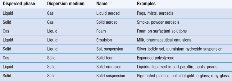
A disperse system consists essentially of one component, the disperse phase, dispersed as particles or droplets throughout another component, the continuous phase. By definition, those dispersions in which the size of the dispersed particles is within the range 10⁻⁹ m (1 nm) to about 10⁻⁶ m (1 µm) are termed colloidal. However, the upper size limit is often extended to include emulsions and suspensions which are very polydisperse systems in which the droplet size frequently exceeds 1 µm, but which show many of the properties of colloidal systems. Some examples of colloidal systems of pharmaceutical interest are shown in Table 5.1. Many natural systems such as suspensions of microorganisms, blood and isolated cells in culture are also colloidal dispersions.

Table 5.1

Types of disperse systems

This chapter will examine the properties of both coarse dispersions, such as emulsions, suspensions and aerosols, and also fine dispersions, such as micellar systems, which fall within the defined size range of true colloidal dispersions.

Colloids can be broadly classified as those that are lyophobic (solvent-hating) and those that are lyophilic (solvent-liking). The terms hydrophobic and hydrophilic are used when the solvent is water. Surfactant molecules tend to associate in water into aggregates called micelles and these constitute hydrophilic colloidal dispersions. Proteins and gums also form lyophilic colloidal systems because of a similar affinity between the dispersed particles and the continuous phase. On the other hand, dispersions of oil droplets in water or water droplets in oil are examples of lyophobic dispersions.

It is because of the subdivision of matter in colloidal systems that they have special properties. A common feature of these systems is a large surface-to-volume ratio of the dispersed particles. As a consequence, there is a tendency for the particles to associate in order to reduce their surface area. Emulsion droplets, for example, eventually coalesce to form a macrophase, so attaining a minimum surface area and hence an equilibrium state. This chapter will examine how the stability of colloidal dispersions can be understood by a consideration of the forces acting between the dispersed particles. Approaches to the formulation of emulsions, suspensions and aerosols will be described and the instability of these coarse dispersions will be discussed using a theory of colloid stability. The association of surface-active agents into micelles and the applications of these colloidal dispersions in the solubilization of poorly water-soluble drugs will also be considered.

Colloids

Preparation of colloidal systems

Lyophilic colloids

The affinity of lyophilic colloids for the dispersion medium leads to the spontaneous formation of colloidal dispersions. For example, acacia, tragacanth, methylcellulose and certain other cellulose derivatives readily disperse in water. This simple method of dispersion is a general one for the formation of lyophilic colloids.

Lyophobic colloids

The preparative methods for lyophobic colloids may be divided into those methods that involve the breakdown of larger particles into particles of colloidal dimensions (dispersion methods) and those in which the colloidal particles are formed by aggregation of smaller particles such as molecules (condensation methods).

Dispersion methods.

The breakdown of coarse material may be carried out by the use of a colloid mill or ultrasonics.

Colloid mills.

These mills cause the dispersion of coarse material by shearing in a narrow gap between a static cone (the stator) and a rapidly rotating cone (the rotor).

Ultrasonic treatment.

The passage of ultrasonic waves through a dispersion medium produces alternating regions of cavitation and compression in the medium. The cavities collapse with great force and cause the breakdown of coarse particles dispersed in the liquid.

With both these methods the particles will tend to reunite unless a stabilizing agent such as a surface-active agent is added.

Condensation methods.

These involve the rapid production of supersaturated solutions of the colloidal material under conditions in which it is deposited in the dispersion medium as colloidal particles and not as a precipitate. The supersaturation is often obtained by means of a chemical reaction that results in the formation of the colloidal material. For example, colloidal silver iodide may be obtained by reacting together dilute solutions of silver nitrate and potassium iodide; colloidal sulphur is produced from sodium thiosulfate and hydrochloric acid solutions; and ferric chloride boiled with excess of water produces colloidal hydrated ferric oxide.

A change of solvent may also cause the production of colloidal particles by condensation methods. If a saturated solution of sulphur in acetone is poured slowly into hot water, the acetone vaporizes, leaving a colloidal dispersion of sulphur. A similar dispersion may be obtained when a solution of a resin, such as benzoin in alcohol, is poured into water.

Purification of colloidal systems

Dialysis

Colloidal particles are not retained by conventional filter papers but are too large to diffuse through the pores of membranes such as those made from regenerated cellulose products, e.g. collodion (cellulose nitrate evaporated from a solution in alcohol and ether) and cellophane. The smaller molecules in solution are able to pass through these membranes. Use is made of this difference in diffusibility to separate micromolecular impurities from colloidal dispersions. The process is known as dialysis. The process of dialysis may be hastened by stirring so as to maintain a high concentration gradient of diffusible molecules across the membrane and by renewing the outer liquid from time to time.

Ultrafiltration.

By applying pressure (or suction), the solvent and small particles may be forced across a membrane whilst the larger colloidal particles are retained. The process is referred to as ultrafiltration. It is possible to prepare membrane filters with known pore size and use of these allows the particle size of a colloid to be determined. However, particle size and pore size cannot be properly correlated because the membrane permeability is affected by factors such as electrical repulsion, when both the membrane and particle carry the same charge, and particle adsorption which can lead to blocking of the pores.

Electrodialysis.

An electric potential may be used to increase the rate of movement of ionic impurities through a dialysing membrane and so provide a more rapid means of purification. The concentration of charged colloidal particles at one side and at the base of the membrane is termed electrodecantation.

Properties of colloids

Size and shape of colloidal particles

Size distribution.

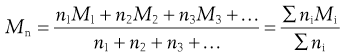
Within the size range of colloidal dimensions specified above, there is often a wide distribution of sizes of the dispersed colloidal particles. The molecular weight or particle size is therefore an average value, the magnitude of which is dependent on the experimental technique used in its measurement. When determined by the measurement of colligative properties such as osmotic pressure, a number average value, M_n, is obtained which, in a mixture containing n₁, n₂, n₃, … moles of particle of mass M₁, M₂, M₃, … respectively, is defined by:

(5.1)

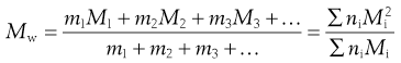
In the light-scattering method for the measurement of particle size, larger particles produce greater scattering and the weight rather than the number of particles is important, giving a weight-average value, M_w, defined by:

(5.2)

In Equation 5.2, m₁, m₂, and m₃ … are the masses of each species, and m_i is obtained by multiplying the mass of each species by the number of particles of that species; that is, m_i = n_iM_i. A consequence is that M_w > M_n, and only when the system is monodisperse will the two averages be identical. The ratio M_w/M_n expresses the degree of polydispersity of the system.

Shape.

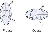
Many colloidal systems, including emulsions, liquid aerosols and most dilute micellar solutions, contain spherical particles. Small deviations from sphericity are often treated using ellipsoidal models. Ellipsoids of revolution are characterized by their axial ratio, which is the ratio of the half-axis a to the radius of revolution b (see Fig. 5.1). Where this ratio is greater than unity, the ellipsoid is said to be a prolate ellipsoid (rugby ball shaped), and when less than unity an oblate ellipsoid (discus-shaped).

Fig. 5.1 Model representation of ellipsoids of revolution.

High molecular weight polymers and naturally occurring macromolecules often form random coils in aqueous solution. Clay suspensions are examples of systems containing plate-like particles.

Kinetic properties

In this section several properties of colloidal systems, which relate to the motion of particles with respect to the dispersion medium, will be considered. Thermal motion manifests itself in the form of Brownian motion, diffusion and osmosis. Gravity (or a centrifugal field) leads to sedimentation. Viscous flow is the result of an externally applied force. Measurement of these properties enables molecular weights or particle size to be determined.

Brownian motion.

Colloidal particles are subject to random collisions with the molecules of the dispersion medium with the result that each particle pursues an irregular and complicated zigzag path. If the particles (up to about 2 µm diameter) are observed under a microscope or the light scattered by colloidal particles is viewed using an ultramicroscope, an erratic motion is seen. This movement is referred to as Brownian motion after Robert Brown who first reported his observation of this phenomenon with pollen grains suspended in water.

Diffusion.

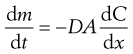
As a result of Brownian motion, colloidal particles spontaneously diffuse from a region of higher concentration to one of lower concentration. The rate of diffusion is expressed by Fick’s First Law. One form of this relationship is shown in Equation 5.3.

(5.3)

where dm is the mass of substance diffusing in time dt across an area A under the influence of a concentration gradient dC/dx (the minus sign denotes that diffusion takes place in the direction of decreasing concentration). D is the diffusion coefficient and has the dimensions of area per unit time. The diffusion coefficient of a dispersed material is related to the frictional coefficient, f, of the particles by Einstein’s Law of Diffusion:

(5.4)

where k_B is the Boltzmann constant and T temperature.

Therefore, as the frictional coefficient is given by the Stokes equation:

(5.5)

where η is the viscosity of the medium and a the radius of the particle (assuming sphericity), then:

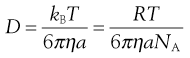(5.6)

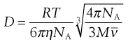
N_A is the Avogadro constant, R is the universal gas constant and k_B = R/N_A. The diffusion coefficient may be obtained by an experiment measuring the change in concentration, via refractive index gradients, when the solvent is carefully layered over the solution to form a sharp boundary and diffusion is allowed to proceed. A more commonly used method is that of dynamic light scattering which is based on the frequency shift of laser light as it is scattered by a moving particle, the so-called Doppler shift. The diffusion coefficient can be used to obtain the molecular weight of an approximately spherical particle, such as egg albumin and haemoglobin, by using Equation 5.5 in the form:

(5.7)

where M is the molecular weight and is the partial specific volume of the colloidal material.

Sedimentation.

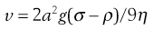
Consider a spherical particle of radius a and density σ falling in a liquid of density ρ and viscosity η. The velocity v of sedimentation is given by Stokes’ Law:

(5.8)

where g is acceleration due to gravity.

If the particles are only subjected to the force of gravity then, due to Brownian motion, the lower size limit of particles obeying Equation 5.8 is about 0.5 µm. A stronger force than gravity is therefore needed for colloidal particles to sediment and use is made of a high-speed centrifuge, usually termed an ultracentrifuge, which can produce a force of about 10⁶ g. In a centrifuge, g is replaced by ω²x, where ω is the angular velocity and x the distance of the particle from the centre of rotation.

The ultracentrifuge is used in two distinct ways in investigating colloidal material. In the sedimentation velocity method, a high centrifugal field is applied, up to about 4 × 10⁵ g, and the movement of the particles, monitored by changes in concentration, is measured at specified time intervals. In the sedimentation equilibrium method, the colloidal material is subjected to a much lower centrifugal field until sedimentation and diffusion tendencies balance one another, and an equilibrium distribution of particles throughout the sample is attained.

Sedimentation velocity.

The velocity dx/dt of a particle in a unit centrifugal force can be expressed in terms of the Svedberg coefficient s:

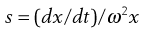(5.9)

Under the influence of the centrifugal force, particles pass from position x₁ at time t₁ to position x₂ at time t₂. The differences in concentration with time can be measured using changes in refractive index and the application of the schlieren optical arrangement, whereby photographs can be taken showing these concentrations as peaks. The expression giving molecular weight M from this method is:

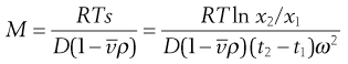(5.10)

where is the partial specific volume of the particle.

Sedimentation equilibrium.

Equilibrium is established when sedimentation and diffusional forces balance.

Combination of sedimentation and diffusion equations is made in the analysis giving:

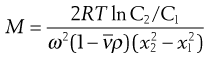(5.11)

where C₁ and C₂ are the sedimentation equilibrium concentrations at distances x₁ and x₂ from the axis of rotation. A disadvantage of the sedimentation equilibrium method is the length of time required to attain equilibrium, often as long as several days. A modification of the method in which measurements are made in the early stages of the approach to equilibrium significantly reduces the overall measurement time.

Osmotic pressure.

The determination of molecular weights of dissolved substances from colligative properties such as the depression of freezing point or the elevation of boiling point is a standard procedure. However, of the available methods, only osmotic pressure has a practical value in the study of colloidal particles because of the magnitude of the changes in the properties. For example, the depression of freezing point of a 1% w/v solution of a macromolecule of molecular weight 70 000 Da is only 0.0026 K, far too small to be measured with sufficient accuracy by conventional methods and also very sensitive to the presence of low molecular weight impurities. In contrast, the osmotic pressure of this solution at 20 °C would be 350 N m⁻² or about 35 mm of water. Not only does the osmotic pressure provide an effect that is measurable, but also the effect of any low molecular weight material, which can pass through the membrane, is virtually eliminated.

However, the usefulness of osmotic pressure measurement is limited to a molecular weight range of about 10⁴−10⁶ Da; below 10⁴ Da the membrane may be permeable to the molecules under consideration and above 10⁶ Da the osmotic pressure will be too small to permit accurate measurement.

If a solution and solvent are separated by a semi-permeable membrane, the tendency to equalize chemical potentials (and hence concentrations) on either side of the membrane results in a net diffusion of solvent across the membrane. The pressure necessary to balance this osmotic flow is termed the osmotic pressure.

For a colloidal solution the osmotic pressure, Π, can be described by:

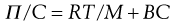(5.12)

where C is the concentration of the solution, M the molecular weight of the solute and B a constant depending on the degree of interaction between the solvent and solute molecules.

Thus a plot of Π/C versus C is linear with the value of the intercept at C → 0 giving RT/M enabling the molecular weight of the colloid to be calculated. The molecular weight obtained from osmotic pressure measurements is a number-average value.

A potential source of error in the determination of molecular weight from osmotic pressure measurements arises from the Donnan membrane effect. The diffusion of small ions through a membrane will be affected by the presence of a charged macromolecule that is unable to penetrate the membrane because of its size. At equilibrium, the distribution of the diffusible ions is unequal, being greater on the side of the membrane containing the non-diffusible ions. Consequently, unless precautions are taken to correct for this effect or eliminate it, the results of osmotic pressure measurements on charged colloidal particles such as proteins will be invalid.

Viscosity.

Viscosity is an expression of the resistance to flow of a system under an applied stress. An equation of flow applicable to colloidal dispersions of spherical particles was developed by Einstein:

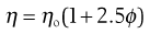(5.13)

where η_o is the viscosity of the dispersion medium and η the viscosity of the dispersion when the volume fraction of colloidal particles present is ϕ.

A number of viscosity coefficients may be defined with respect to Equation 5.13. These include relative viscosity:

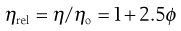(5.14)

and specific viscosity:

(5.15)

Since volume fraction is directly related to concentration, Equation 5.15 may be written as:

(5.16)

where C is the concentration expressed as grams of colloidal particles per 100 mL of total dispersion and k is a constant. If η is determined for a number of concentrations of macromolecular material in solution and η_sp/C is plotted versus C then the intercept obtained on extrapolation of the linear plot to infinite dilution is known as the intrinsic viscosity [η].

This constant may be used to calculate the molecular weight of the macromolecular material by making use of the Mark–Houwink equation:

(5.17)

where K and α are constants characteristic of the particular polymer-solvent system. These constants are obtained initially by determining [η] for a polymer fraction whose molecular weight has been determined by another method such as sedimentation, osmotic pressure or light scattering. The molecular weight of the unknown polymer fraction may then be calculated. This method is suitable for use with polymers, such as dextrans used as blood plasma substitutes.

Optical properties

Light scattering.

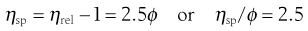
When a beam of light is passed through a colloidal sol (dispersion of very fine particles), some of the light may be absorbed (when light of certain wavelengths is selectively absorbed, a colour is produced), some is scattered and the remainder is transmitted undisturbed through the sample. Due to the light scattered, the sol appears turbid; this is known as the Tyndall effect. The turbidity of a sol is given by the expression:

(5.18)

where I_o is the intensity of the incident beam, I that of the transmitted light beam, l the length of the sample and τ the turbidity.

Light-scattering measurements are of great value for estimating particle size, shape and interactions, particularly of dissolved macromolecular materials, as the turbidity depends on the size (molecular weight) of the colloidal material involved. Measurements are simple in principle but experimentally difficult because of the need to keep the sample free from dust, the particles of which would scatter light strongly and introduce large errors.

As most colloids show very low turbidities, instead of measuring the transmitted light (which may differ only marginally from the incident beam), it is more convenient and accurate to measure the scattered light, at an angle (usually 90°) relative to the incident beam. The turbidity can then be calculated from the intensity of the scattered light, provided the dimensions of the particle are small compared to the wavelength of the incident light, by the expression:

(5.19)

R₉₀ is known as the Rayleigh ratio after Lord Rayleigh who laid the foundations of the light-scattering theory. The light-scattering theory was modified for use in the determination of the molecular weight of colloidal particles by Debye who derived the following relationship between turbidity and molecular weight:

(5.20)

C is the concentration of the solute and B an interaction constant allowing for non-ideality. H is an optical constant for a particular system depending on the refractive index change with concentration and the wavelength of light used. A plot of HC/τ against concentration results in a straight line of slope 2B. The intercept on the HC/τ axis is 1/M, allowing the molecular weight to be calculated. The molecular weight derived by the light-scattering technique is a weight-average value.

Light-scattering measurements are particularly suitable for finding the size of the micelles of surface-active agents and for the study of proteins and natural and synthetic polymers.

For spherical particles, the upper limit of the Debye equation is a particle diameter of approximately one-twentieth of the wavelength λ of the incident light; that is, about 20–25 nm. The light-scattering theory becomes more complex when one or more dimensions exceed λ/20 because the particles can no longer be considered as point sources of scattered light. By measuring the light scattering from such particles as a function of both the scattering angle θ and the concentration C, and extrapolating the data to zero angle and zero concentration, it is possible to obtain information on not only the molecular weight but also the particle shape.

Because the intensity of the scattered light is inversely proportional to the fourth power of the wavelength of the light used, blue light (λ = 450 nm) is scattered much more than red light (λ = 650 nm). With incident white light, a scattering material will therefore tend to be blue when viewed at right angles to the incident beam, which is why the sky appears to be blue, the scattering arising from dust particles in the atmosphere.

Ultramicroscopy.

Colloidal particles are too small to be seen with an optical microscope. Light scattering is employed in the ultramicroscope first developed by Zsigmondy, in which a cell containing the colloid is viewed against a dark background at right angles to an intense beam of incident light. The particles, which exhibit Brownian motion, appear as spots of light against the dark background. The ultramicroscope is used in the technique of microelectrophoresis for measuring particle charge.

Electron microscopy.

The electron microscope, capable of giving actual pictures of the particles, is used to observe the size, shape and structure of colloidal particles. The success of the electron microscope is due to its high resolving power, defined in terms of d, the smallest distance by which two objects are separated yet remain distinguishable. The smaller the wavelength of the radiation used, the smaller is d and the greater the resolving power. An optical microscope, using visible light as its radiation source, gives a d of about 0.2 µm. The radiation source of the electron microscope is a beam of high-energy electrons having wavelengths in the region of 0.01 nm; d is thus about 0.5 nm. The electron beams are focused using electromagnets and the whole system is under a high vacuum of about 10⁻³–10⁻⁵ Pa to give the electrons a free path. With wavelengths of the order indicated, the image cannot be viewed directly, so the image is displayed on a monitor or computer screen.

A major disadvantage of the electron microscope for viewing colloidal particles is that normally only dried samples can be examined. Consequently, it usually gives no information on solvation or configuration in solution and, moreover, the particles may be affected by sample preparation. A recent development which overcomes these problems is environmental scanning electron microscopy (ESEM) which allows the observation of material in the wet state.

Electrical properties

Electrical properties of interfaces.

Most surfaces acquire a surface electric charge when brought into contact with an aqueous medium, the principal charging mechanisms being as follows.

Ion dissolution.

Ionic substances can acquire a surface charge by virtue of unequal dissolution of the oppositely charged ions of which they are composed. For example, the particles of silver iodide in a solution with excess [I⁻] will carry a negative charge, but the charge will be positive if excess [Ag⁺] is present. Since the concentrations of Ag⁺ and I⁻ determine the electric potential at the particle surface, they are termed potential-determining ions. In a similar way, H⁺ and OH⁻ are potential-determining ions for metal oxides and hydroxides of, for example, magnesium and aluminium hydroxides.

Ionization.

Here the charge is controlled by the ionization of surface groupings; examples include the model system of polystyrene latex which frequently has carboxylic acid groupings at the surface which ionize to give negatively charged particles. In a similar way, acidic drugs such as ibuprofen and nalidixic acid also acquire a negative charge.

Amino acids and proteins acquire their charge mainly through the ionization of carboxyl and amino groups to give —COO⁻ and NH₃⁺ ions. The ionization of these groups and so the net molecular charge depends on the pH of the system. At a pH below the pK_a of the COO⁻ group the protein will be positively charged because of the protonation of this group, —COO^— → COOH, and the ionization of the amino group, —NH₂ → —NH₃⁺, which has a much higher pK_a. At higher pH, where the amino group is no longer ionized, the net charge on the molecule is negative because of the ionization of the carboxyl group. At a certain definite pH, specific for each individual protein, the total number of positive charges will equal the total number of negative charges and the net charge will be zero. This pH is termed the isoelectric point of the protein and the protein exists as its zwitterion. This may be represented as follows:

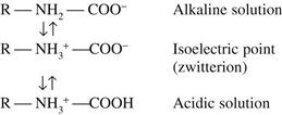
A protein is least soluble (the colloidal sol is least stable) at its isoelectric point and is readily desolvated by very water-soluble salts such as ammonium sulfate. Thus insulin may be precipitated from aqueous alcohol at pH 5.2.

Ion adsorption.

A net surface charge can be acquired by the unequal adsorption of oppositely charged ions. Surfaces in water are more often negatively charged than positively charged, because cations are generally more hydrated than anions. Consequently, the former have the greater tendency to reside in the bulk aqueous medium whereas the smaller, less hydrated and more polarizing anions have the greater tendency to reside at the particle surface. Surface-active agents are strongly adsorbed and have a pronounced influence on the surface charge, imparting either a positive or negative charge depending on their ionic character.

The electrical double layer.

Consider a solid charged surface in contact with an aqueous solution containing positive and negative ions. The surface charge influences the distribution of ions in the aqueous medium; ions of opposite charge to that of the surface, termed counter-ions, are attracted towards the surface, ions of like charge, termed co-ions, are repelled away from the surface. However, the distribution of the ions will also be affected by thermal agitation which will tend to redisperse the ions in solution. The result is the formation of an electrical double layer made up of the charged surface and a neutralizing excess of counter-ions over co-ions (the system must be electrically neutral) distributed in a diffuse manner in the aqueous medium.

The theory of the electric double layer deals with this distribution of ions and hence with the magnitude of the electric potentials which occur in the locality of the charged surface. For a fuller explanation of what is a rather complicated mathematical approach, the reader is referred to a textbook of colloid science (e.g. Shaw 1992). A somewhat simplified picture of what pertains from the theories of Gouy, Chapman and Stern follows.

The double layer is divided into two parts (see Fig. 5.2a): the inner, which may include adsorbed ions, and the diffuse part where ions are distributed as influenced by electrical forces and random thermal motion. The two parts of the double layer are separated by a plane, the Stern plane, at about a hydrated ion radius from the surface; thus counter-ions may be held at the surface by electrostatic attraction and the centre of these hydrated ions forms the Stern plane.

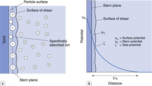
Fig. 5.2 The electric double layer. (a) Schematic representation. (b) Changes in potential with distance from particle surface.

The potential changes linearly from ψ_o (the surface potential) to ψ_δ, (the Stern potential) in the Stern layer and decays exponentially from ψ_δ to zero in the diffuse double layer (Fig. 5.2b). A plane of shear is also indicated in Figure 5.2. In addition to ions in the Stern layer, a certain amount of solvent will be bound to the ions and the charged surface. This solvating layer is held to the surface, and the edge of the layer, termed the surface or plane of shear, represents the boundary of relative movement between the solid (and attached material) and the liquid. The potential at the plane of shear is termed the zeta, ζ, or electrokinetic, potential and its magnitude may be measured using microelectrophoresis or any other of the electrokinetic phenomena. The thickness of the solvating layer is ill-defined and the zeta potential therefore represents a potential at an unknown distance from the particle surface; its value, however, is usually taken as being slightly less than that of the Stern potential.

In the discussion above, it was stated that the Stern plane existed at a hydrated ion radius from the particle surface; the hydrated ions are electrostatically attracted to the particle surface. It is possible for ions/molecules to be more strongly adsorbed at the surface, termed specific adsorption, than by simple electrostatic attraction. In fact, the specifically adsorbed ion/molecule may be uncharged as is the case with non-ionic surface-active agents. Surface-active ions specifically adsorb by the hydrophobic effect and can have a significant effect on the Stern potential, causing ψ_o and ψ_δ to have opposite signs, as in Figure 5.3a, or for ψ_δ to have the same sign as ψ_o but be greater in magnitude, as in Figure 5.3b.

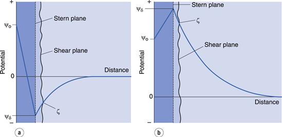
Fig. 5.3 Changes in potential with distance from solid surface. (a) Reversal of charge sign of Stern potential ψ_δ, due to adsorption of surface-active or polyvalent counter-ion. (b) Increase in magnitude of Stern potential ψ_δ, due to adsorption of surface-active co-ions.

Figure 5.2b shows an exponential decay of the potential to zero with distance from the Stern plane. The distance over which this occurs is 1/κ, referred to as the Debye–Hückel length parameter or the thickness of the electrical double layer. The parameter κ is dependent on the electrolyte concentration of the aqueous media. Increasing the electrolyte concentration increases the value of κ and consequently decreases the value of 1/κ; that is, it compresses the double layer. As ψ_δ stays constant this means that the zeta potential will be lowered.

As indicated earlier, the effect of specifically adsorbed ions may be to lower the Stern potential and hence the zeta potential without compressing the double layer. Thus the zeta potential may be reduced by additives to the aqueous system in either (or both) of two different ways.

Electrokinetic phenomena.

This is the general description applied to the phenomena that arise when attempts are made to shear off the mobile part of the electrical double layer from a charged surface. There are four such phenomena: namely, electrophoresis, sedimentation potential, streaming potential and electroosmosis. All of these electrokinetic phenomena may be used to measure the zeta potential but electrophoresis is the easiest to use and has the greatest pharmaceutical application.

Electrophoresis.

The movement of a charged particle (plus attached ions) relative to a stationary liquid under the influence of an applied electric field is termed electrophoresis. When the movement of the particles is observed with a microscope, or the movement of light spots scattered by particles too small to be observed with the microscope is observed using an ultramicroscope, this constitutes microelectrophoresis.

A microscope equipped with an eyepiece graticule is used and the speed of movement of the particle under the influence of a known electric field is measured. This is the electrophoretic velocity, v, and the electrophoretic mobility, u, is given by:

(5.21)

where v is measured in m s⁻¹, and E, the applied field strength, in V m⁻¹, so that u has the dimensions of m² s⁻¹ V⁻¹. Typically, a stable lyophobic colloidal particle may have an electrophoretic mobility of 4 × 10⁻⁸ m² s⁻¹ V⁻¹. The equation used for converting the electrophoretic mobility, u, into the zeta potential depends on the value of κa (κ is the Debye–Hückel reciprocal length parameter described previously and a the particle radius). For values of κa > 100 (as is the case for particles of radius 1 µm dispersed in 10⁻³ mol dm⁻³ sodium chloride solution) the Smoluchowski equation can be used:

(5.22)

where ε is the permittivity and η the viscosity of the liquid used. For particles in water at 25 °C, ζ = 12.85 × 10⁻⁵ u volts and, for the mobility given above, a zeta potential of 0.0514 volts or 51.4 millivolts is obtained. For values of κa < 100, a more complex relationship which is a function of κa and the zeta potential is used.

The technique of microelectrophoresis finds application in the measurement of zeta potentials, of model systems (like polystyrene latex dispersions) to test colloid stability theory, of coarse dispersions (like suspensions and emulsions) to assess their stability, and in identification of charge groups and other surface characteristics of water-insoluble drugs and cells such as blood and bacteria.

Other electrokinetic phenomena The other electrokinetic phenomena are as follows. Sedimentation potential, the reverse of electrophoresis, is the electric field created when particles sediment; streaming potential, the electric field created when liquid is made to flow along a stationary charged surface, e.g. a glass tube or a packed powder bed; and electroosmosis, the opposite of streaming potential, the movement of liquid relative to a stationary charged surface, e.g. a glass tube, by an applied electric field.

Physical stability of colloidal systems

In colloidal dispersions, frequent encounters between the particles occur due to Brownian movement. Whether these collisions result in permanent contact of the particles (coagulation), which leads eventually to the destruction of the colloidal system as the large aggregates formed sediment out, or temporary contact (flocculation) or whether the particles rebound and remain freely dispersed (a stable colloidal system) depends on the forces of interaction between the particles.

These forces can be divided into three groups: electrical forces of repulsion, forces of attraction and forces arising from solvation. An understanding of the first two explains the stability of lyophobic systems, and all three forces must be considered in a discussion of the stability of lyophilic dispersions. Before considering the interaction of these forces, it is necessary to define the terms aggregation, coagulation and flocculation as used in colloid science.

Aggregation is a general term signifying the collection of particles into groups. Coagulation signifies that the particles are closely aggregated and difficult to redisperse – a primary minimum phenomenon of the DLVO theory of colloid stability (see next section). In flocculation, the aggregates have an open structure in which the particles remain a small distance apart from one another. This may be a secondary minimum phenomenon (see the DLVO theory) or a consequence of bridging by a polymer or polyelectrolyte, as explained later in this chapter.

As a preliminary to discussion on the stability of colloidal dispersions, a comparison of the general properties of lyophobic and lyophilic sols is given in Table 5.2.

Table 5.2

Comparison of properties of lyophobic and lyophilic sols

Property	Lyophobic	Lyophilic
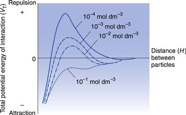
Effect of electrolytes	Very sensitive to added electrolyte, leading to aggregation in an irreversible manner. Depends on: (a) type and valency of counter ion of electrolyte, e.g. with a negatively charged sol. La³⁺ > Ba²⁺ > Na⁺ (b) Concentration of electrolyte. At a particular concentration sol passes from disperse to aggregated state. For the electrolyte types in (a) the concentrations are about 10⁻⁴, 10⁻³, 10⁻¹ mol dm⁻³ respectively. These generalizations, (a) and (b), form what is known as the Schulze−Hardy rule	Dispersions are stable generally in the presence of electrolytes. May be salted out by high concentrations of very soluble electrolytes. Effect is due to desolvation of the lyophilic molecules and depends on the tendency of the electrolyte ions to become hydrated. Proteins more sensitive to electrolytes at their isoelectric points. Lyophilic colloids when salted out may appear as amorphous droplets known as a coacervate
Stability	Controlled by charge on particles	Controlled by charge and solvation of particles
Formation of dispersion	Dispersions usually of metals, inorganic crystals, etc., with a high interfacial surface-free energy due to large increase in surface area on formation. A positive ΔG of formation, dispersion will never form spontaneously and is thermodynamically unstable. Particles of sol remain dispersed due to electrical repulsion	Generally proteins, macromolecules, etc., which disperse spontaneously in a solvent. Interfacial free energy is low. There is a large increase in entropy when rigidly held chains of a polymer in the dry state unfold in solution. The free energy of formation is negative, a stable thermodynamic system
Viscosity	Sols of low viscosity, particles unsolvated and usually symmetrical	Usually high. At sufficiently high concentration of disperse phase a gel may be formed. Particles solvated and usually asymmetric

Stability of lyophobic systems (DLVO theory).

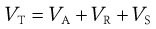
In considering the interaction between two colloidal particles, Derjaguin and Landau and, independently, Verwey and Overbeek in the 1940s produced a quantitative approach to the stability of hydrophobic sols. In what has come to be known as the DLVO theory of colloid stability, they assumed that the only interactions involved are electrical repulsion, V_R, and van der Waals attraction, V_A, and that these parameters are additive. Therefore the total potential energy of interaction V_T (expressed schematically in the curve shown in Fig. 5.4) is given by:

(5.23)

Fig. 5.4 Schematic curve of total potential energy of interaction, V_T, versus distance of separation, H, for two particles. V_T = V_R + V_A.

Repulsive forces between particles.

Repulsion between particles arises due to the osmotic effect produced by the increase in the number of charged species on overlap of the diffuse parts of the electrical double layer. No simple equations can be given for repulsive interactions; however, it can be shown that the repulsive energy that exists between two spheres of equal but small surface potential is given by:

(5.24)

where ε is the permittivity of the polar liquid, a the radius of the spherical particle of surface potential ψ_o, κ is the Debye–Hückel reciprocal length parameter and H the distance between particles. An estimation of the surface potential can be obtained from zeta potential measurements. As can be seen, the repulsion energy is an exponential function of the distance between the particles and has a range of the order of the thickness of the double layer.

Attractive forces between particles.

The energy of attraction, V_A, arises from van der Waals universal forces of attraction, the so-called dispersion forces, the major contribution to which are the electromagnetic attractions described by London. For an assembly of molecules, dispersion forces are additive, summation leading to long-range attraction between colloidal particles. As a result of the work of de Boer and Hamaker, it can be shown that the attractive interaction between spheres of the same radius, a, can be approximated to:

(5.25)

where A is the Hamaker constant for the particular material derived from London dispersion forces. Equation 5.25 shows that the energy of attraction varies as the inverse of the distance between particles, H.

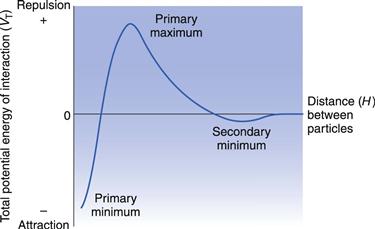
Total potential energy of interaction.

Consideration of the curve of total potential energy of interaction V_T versus distance between particles, H (Fig. 5.4), shows that attraction predominates at small distances, hence the very deep primary minimum. The attraction at large interparticle distances, that produces the secondary minimum, arises because the fall-off in repulsive energy with distance is more rapid than that of attractive energy. At intermediate distances, double layer repulsion may predominate, giving a primary maximum in the curve. If this maximum is large compared with the thermal energy k_BT of the particles, the colloidal system should be stable, i.e. the particles should stay dispersed. Otherwise, the interacting particles will reach the energy depth of the primary minimum and irreversible aggregation, i.e. coagulation, occurs. If the secondary minimum is smaller than k_BT the particles will not aggregate but will always repel one another, but if it is significantly larger than k_BT a loose assemblage of particles will form which can be easily redispersed by shaking, i.e. flocculation occurs.

The depth of the secondary minimum depends on particle size, and particles may need to be of radius 1 µm or greater before the attractive force is sufficiently great for flocculation to occur.

The height of the primary maximum energy barrier to coagulation depends upon the magnitude of V_R, which is dependent on ψ_o and hence the zeta potential. In addition, it depends on electrolyte concentration via κ, the Debye–Hückel reciprocal length parameter. Addition of electrolyte compresses the double layer and reduces the zeta potential; this has the effect of lowering the primary maximum and deepening the secondary minimum (Fig. 5.5). This latter means that there will be an increased tendency for particles to flocculate in the secondary minimum and this is the principle of the controlled flocculation approach to pharmaceutical suspension formulation described later. The primary maximum may also be lowered (and the secondary minimum deepened) by adding substances, such as ionic surface-active agents, which are specifically adsorbed within the Stern layer. Here ψ_δ is reduced and hence the zeta potential; the double layer is usually not compressed.

Fig. 5.5 Schematic curves of total potential energy of interaction, V_T, versus distance of separation, H, showing the effect of adding electrolyte at constant surface potential.

Stability of lyophilic systems.

Solutions of macromolecules, lyophilic colloidal sols, are stabilized by a combination of electrical double layer interaction and solvation and both of these stabilizing factors must be sufficiently weakened before attraction predominates and the colloidal particles coagulate. For example, gelatin has a sufficiently strong affinity for water to be soluble even at its isoelectric pH where there is no double layer interaction.

Hydrophilic colloids are unaffected by the small amounts of added electrolyte which cause hydrophobic sols to coagulate. However, when the concentration of electrolyte is high, particularly with an electrolyte whose ions become strongly hydrated, the colloidal material loses its water of solvation to these ions and coagulates, i.e. a ‘salting out’ effect occurs.

Variation in the degree of solvation of different hydrophilic colloids affects the concentration of soluble electrolyte required to produce their coagulation and precipitation. The components of a mixture of hydrophilic colloids can therefore be separated by a process of fractional precipitation, which involves the ‘salting out’ of the various components at different concentrations of electrolyte. This technique is used in the purification of antitoxins.

Lyophilic colloids can be considered to become lyophobic by the addition of solvents such as acetone and alcohol. The particles become desolvated and are then very sensitive to precipitation by added electrolyte.

Coacervation and microencapsulation.

Coacervation is the separation of a colloid-rich layer from a lyophilic sol as the result of the addition of another substance. This layer, which is present in the form of an amorphous liquid, constitutes the coacervate. Simple coacervation may be brought about by a ‘salting out’ effect on addition of electrolyte or addition of a non-solvent. Complex coacervation occurs when two oppositely charged lyophilic colloids are mixed, e.g. gelatin and acacia. Gelatin at a pH below its isoelectric point is positively charged, acacia above about pH 3 is negatively charged; a combination of solutions at about pH 4 results in coacervation. Any large ions of opposite charge, for example cationic surface-active agents (positively charged) and dyes used for colouring aqueous mixtures (negatively charged), may react in a similar way.

If the coacervate is formed in a stirred suspension of an insoluble solid, the macromolecular material will surround the solid particles. The coated particles can be separated and dried and this technique forms the basis of one method of microencapsulation. A number of drugs including aspirin have been coated in this manner. The coating protects the drug from chemical attack and microcapsules may be given orally to prolong the action of the medicament.

Effect of addition of macromolecular material to lyophobic colloidal sols.

When added in small amounts, many polyelectrolyte and polymer molecules (lyophilic colloids) can adsorb simultaneously on to two particles and are long enough to bridge across the energy barrier between the particles. This can even occur with neutral polymers when the lyophobic particles have a high zeta potential (and would thus be considered a stable sol). A structured floc results (Fig. 5.6a).

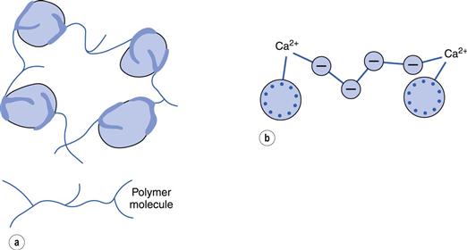
Fig. 5.6 Diagram of flocs formed by (a) polymer bridging and (b) polyelectrolyte bridging in the presence of divalent ions of opposite charge.

With polyelectrolytes, where the particles and polyelectrolyte have the same sign, flocculation can often occur when divalent and trivalent ions are added to the system (Fig. 5.6b). These complete the ‘bridge’ and only very low concentrations of these ions are needed. Use is made of this property of small quantities of polyelectrolytes and polymers in removing colloidal material, resulting from sewage, in water purification.

On the other hand, if larger amounts of polymer are added, sufficient to cover the surface of the particles, then a lyophobic sol may be stabilized to coagulation by added electrolyte – the so-called steric stabilization or protective colloid effect.

Steric stabilization (protective colloid action).

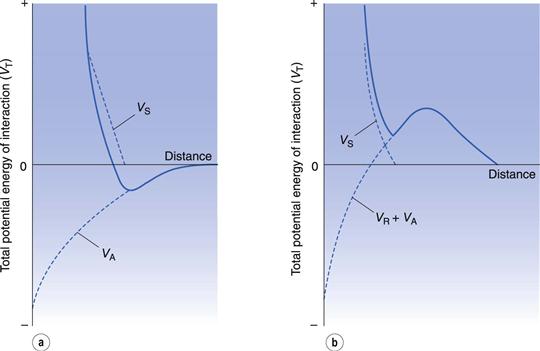
It has long been known that non-ionic polymeric materials such as gums, non-ionic surface-active agents and methylcellulose adsorbed at the particle surface can stabilize a lyophobic sol to coagulation even in the absence of a significant zeta potential. The approach of two particles with adsorbed polymer layers results in a steric interaction when the layers overlap, leading to repulsion. In general, the particles do not approach each other closer than about twice the thickness of the adsorbed layer and hence passage into the primary minimum is inhibited. An additional term has thus to be included in the potential energy of interaction for what is called steric stabilization, V_S:

(5.26)

The effect of V_S on the potential energy against distance between particles is seen in Figure 5.7, showing that repulsion is generally seen at all shorter distances provided that the adsorbed polymeric material does not move from the particle surface.

Fig. 5.7 Schematic curves of the total potential energy of interaction versus distance for two particles, showing the effect of the steric stabilization term V_S (a) in the absence of electrostatic repulsion, the solid line representing V_T = V_A + V_S; (b) in the presence of electrostatic repulsion, the solid line representing V_T = V_R + V_A + V_S.

Steric repulsion can be explained by reference to the free energy changes that take place when two polymer-covered particles interact. Free energy ΔG, enthalpy ΔH and entropy ΔS changes are related according to:

(5.27)

The Second Law of Thermodynamics implies that a positive value of ΔG is necessary for dispersion stability, a negative value indicating that the particles have aggregated.

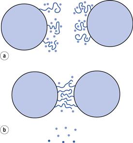
A positive value of ΔG can arise in a number of ways, for example when ΔH and ΔS are both negative and TΔS > ΔH. Here the effect of the entropy change opposes aggregation and outweighs the enthalpy term; this is termed entropic stabilization. Interpenetration and compression of the polymer chains decrease the entropy as these chains become more ordered. Such a process is not spontaneous: ‘work’ must be expended to interpenetrate and compress any polymer chains existing between the colloidal particles and this work is a reflection of the repulsive potential energy. The enthalpy of mixing of these polymer chains will also be negative. Stabilization by these effects occurs in non-aqueous dispersions.

Again, a positive ΔG occurs if both ΔH and ΔS are positive and TΔS < ΔH. Here enthalpy aids stabilization, entropy aids aggregation. Consequently, this effect is termed enthalpic stabilization and is common with aqueous dispersions, particularly where the stabilizing polymer has polyoxyethylene chains. Such chains are hydrated in aqueous solution due to H-bonding between water molecules and the ‘ether oxygens’ of the ethylene oxide groups. The water molecules have thus become more structured and lost degrees of freedom. When interpenetration and compression of ethylene oxide chains occur, there is an increased probability of contact between ethylene oxide groups, resulting in some of the bound water molecules being released (see Fig. 5.8). The released water molecules have greater degrees of freedom than those in the bound state. For this to occur, they must be supplied with energy, obtained from heat absorption, i.e. there is a positive enthalpy change. Although there is a decrease in entropy in the interaction zone, as with entropic stabilization, this is overridden by the increase in the configurational entropy of the released water molecules.

Fig. 5.8 Enthalpic stabilization. (a) Particles with stabilizing polyoxyethylene chains and H-bonded water molecules. (b) Stabilizing chains overlap, water molecules released → + ΔH.

Gels

The majority of gels are formed by aggregation of colloidal sol particles; the solid or semi-solid system so formed being interpenetrated by a liquid. The particles link together to form an interlaced network, thus imparting rigidity to the structure; the continuous phase is held within the meshes. Often only a small percentage of disperse phase is required to impart rigidity; for example, 1% of agar in water produces a firm gel. A gel rich in liquid may be called a jelly; if the liquid is removed and only the gel framework remains, this is termed a xerogel. Sheet gelatin, acacia tears and tragacanth flakes are all xerogels.

Types of gel

Gelation of lyophobic sols

Gels may be flocculated lyophobic sols where the gel can be looked upon as a continuous floccule (Fig. 5.9a). Examples are aluminium hydroxide and magnesium hydroxide gels.

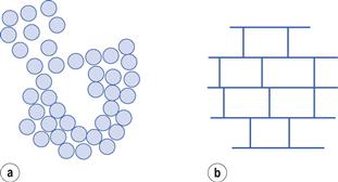
Fig. 5.9 Gel structure. (a) Flocculated lyophobic sol, e.g. aluminium hydroxide. (b) ‘Card house’ floc of clays, e.g. bentonite.

Clays such as bentonite, aluminium magnesium silicate (Veegum) and to some extent kaolin form gels by flocculation in a special manner. They are hydrated aluminium (aluminium/magnesium) silicates whose crystal structure is such that they exist as flat plates. The flat part or ‘face’ of the particle carries a negative charge due to O⁻ atoms and the edge of the plate carries a positive charge due to Al³⁺/Mg²⁺ atoms. As a result of electrostatic attraction between the face and edge of different particles, a gel structure is built up, forming what is usually known as a ‘card house floc’ (Fig. 5.9b).

The forces holding the particles together in this type of gel are relatively weak – van der Waals forces in the secondary minimum flocculation of aluminium hydroxide, electrostatic attraction in the case of the clays. Because of this these gels show the phenomenon of thixotropy, a non-chemical isothermal gel-sol-gel transformation. If a thixotropic gel is sheared (for example, by simple shaking) these weak bonds are broken and a lyophobic sol is formed. On standing, the particles collide, flocculation occurs and the gel is reformed. Flocculation in gels is the reason for their anomalous rheological properties (see Chapter 6). This phenomenon of thixotropy is employed in the formulation of pharmaceutical suspensions, e.g. bentonite in calamine lotion, and in the paint industry.

Gelation of lyophilic sols

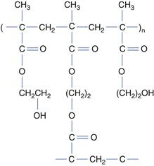
Gels formed by lyophilic sols can be divided into two groups depending on the nature of the bonds between the chains of the network. Gels of type I are irreversible systems with a three-dimensional network formed by covalent bonds between the macromolecules. Typical examples of this type of gel are the swollen networks that have been formed by the polymerization of monomers of water-soluble polymers in the presence of a cross-linking agent. For example, poly (2-hydroxyethylmethacrylate) [poly(HEMA)], crosslinked with ethylene glycol dimethacrylate [EGDMA], forms a three-dimensional structure (Fig. 5.10), that swells in water but cannot dissolve because the crosslinks are stable. Such polymers have been used in the fabrication of expanding implants that imbibe body fluids and swell to a predetermined volume. Implanted in the dehydrated state, these polymers swell to fill a body cavity or give form to surrounding tissues. They also find use in the fabrication of implants for the prolonged release of drugs, such as antibiotics, into the immediate environment of the implant.

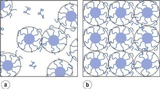
Fig. 5.10 Poly(HEMA): poly(2-hydroxyethyl methacrylate) crosslinked with ethylene glycol dimethacrylate (EGDMA).

Type II gels are held together by much weaker intermolecular bonds such as hydrogen bonds. These gels are heat reversible, a transition from the sol to gel occurring on either heating or cooling. Poly(vinyl alcohol) solutions, for example, gel on cooling below a certain temperature referred to as the gel point. Because of their gelling properties, poly(vinyl alcohol)s are used as jellies for application of drugs to the skin. On application, the gel dries rapidly, leaving a plastic film with the drug in intimate contact with the skin. Concentrated aqueous solutions of high molecular weight poly(oxyethylene)-poly(oxypropylene)-poly(oxyethylene) block copolymers, commercially available as Pluronic™ or Synperonic™ surfactants, form gels on heating. These compounds are amphiphilic and many form micelles with a hydrophobic core comprising the poly(oxypropylene) blocks, surrounded by a shell of the hydrophilic poly(oxyethylene) chains. Unusually, water is a poorer solvent for these compounds at higher temperatures and consequently warming a solution with a concentration above the critical micelle concentration leads to the formation of more micelles. If the solution is sufficiently concentrated gelation may occur as the micelles pack so closely as to prevent their movement (see Fig. 5.11). Gelation is a reversible process, the gels returning to the sol state on cooling.

Fig. 5.11 Poly(oxyethylene)-poly(oxypropylene)-poly(oxyethylene) block copolymers. (a) Micelle formation. (b) Formation of a cubic gel phase by packing of micelles.

Surface-active agents

Certain compounds, because of their chemical structure, have a tendency to accumulate at the boundary between two phases (see Chapter 4 for further information on surfaces and interfaces). Such compounds are termed amphiphiles, surface-active agents or surfactants. The adsorption at the various interfaces between solids, liquids and gases results in changes in the nature of the interface which are of considerable importance in pharmacy. Thus, the lowering of the interfacial tension between oil and water phases facilitates emulsion formation, the adsorption of surfactants on insoluble particles enables these particles to be dispersed in the form of a suspension, their adsorption on solid surfaces enables these surfaces to be more readily wetted, and the incorporation of insoluble compounds within micelles of the surfactant can lead to the production of clear solutions.

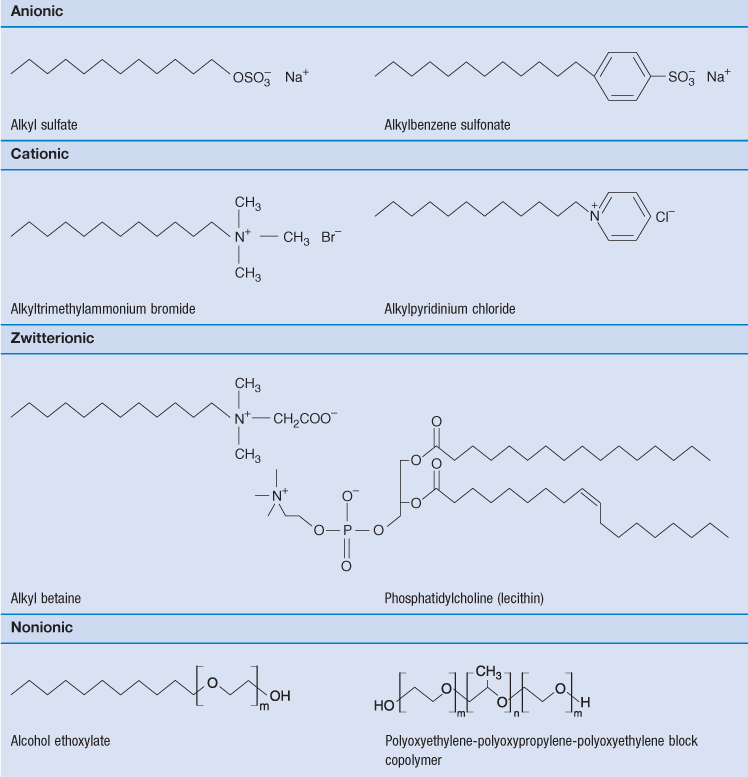
Surface-active compounds are characterized by having two distinct regions in their chemical structure, one hydrophilic (water-liking) and the other hydrophobic (water-hating) regions. The existence of two such regions in a molecule is referred to as amphipathy and the molecules are consequently often referred to as amphipathic molecules. The hydrophobic portions are usually saturated or unsaturated hydrocarbon chains or, less commonly, heterocyclic or aromatic ring systems. The hydrophilic regions can be anionic, cationic or non-ionic. Surfactants are generally classified according to the nature of the hydrophilic group. Typical examples are given in Table 5.3.

Table 5.3

Classification of surface-active agents

Many water-soluble drugs have also been reported to be surface active, this surface activity being a consequence of the amphipathic nature of the drugs. The hydrophobic portions of the drug molecules are usually more complex than those of typical surface-active agents, being composed of aromatic or heterocyclic ring systems. Examples include tranquillizers such as chlorpromazine which are based on the large tricyclic phenothiazine ring system; antidepressant drugs such as imipramine which also possess tricyclic ring systems; and antihistamines such as diphenhydramine which are based on a diphenylmethane group. Further examples of surface-active drugs are given in Attwood & Florence (1983).

Surface activity

The dual structure of amphipathic molecules is the unique feature that is responsible for the surface activity of these compounds. It is a consequence of their adsorption at the solution–air interface, the means by which the hydrophobic region of the molecule ‘escapes’ from the hostile aqueous environment by protruding into the vapour phase above. Similarly, adsorption at the interface between water and an immiscible non-aqueous liquid occurs in such a way that the hydrophobic group is in solution in the non-aqueous phase, leaving the hydrophilic group in contact with the aqueous solution.

As discussed in Chapter 4, the molecules at the surface of a liquid are not completely surrounded by other like molecules as they are in the bulk of the liquid. As a result there is a net inward force of attraction exerted on a molecule at the surface from the molecules in the bulk solution, which results in a tendency for the surface to contract. The contraction of the surface is spontaneous; that is, it is accompanied by a decrease in free energy. The contracted surface thus represents a minimum free energy state and any attempt to expand the surface must involve an increase in the free energy. The surface tension is a measure of the contracting power of the surface. Surface-active molecules in aqueous solution orientate themselves at the surface in such a way as to remove the hydrophobic group from the aqueous phase and hence achieve a minimum free energy state. As a result, some of the water molecules at the surface are replaced by non-polar groups. The attractive forces between these groups and the water molecules, or between the groups themselves, are less than those existing between water molecules. The contracting power of the surface is thus reduced and so therefore is the surface tension.

A similar imbalance of attractive forces exists at the interface between two immiscible liquids. The value of the interfacial tension is generally between those of the surface tensions of the two liquids involved except where there is interaction between them. Intrusion of surface-active molecules at the interface between two immiscible liquids leads to a reduction of interfacial tension, in some cases to such a low level that spontaneous emulsification of the two liquids occurs.

Micelle formation

The surface tension of a surfactant solution decreases progressively with increase of concentration as more surfactant molecules enter the surface or interfacial layer. However, at a certain concentration this layer becomes saturated and an alternative means of shielding the hydrophobic group of the surfactant from the aqueous environment occurs through the formation of aggregates (usually spherical) of colloidal dimensions, called micelles. The hydrophobic chains form the core of the micelle and are shielded from the aqueous environment by the surrounding shell composed of the hydrophilic groups that serve to maintain solubility in water.

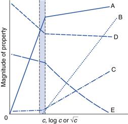
The concentration at which micelles first form in solution is termed the critical micelle concentration or CMC. This onset of micelle formation can be detected by a variety of experimental techniques. When physical properties such as surface tension, conductivity, osmotic pressure, solubility and light-scattering intensity are plotted as a function of concentration (see Fig. 5.12) a change of slope occurs at the CMC and such techniques can be used to measure its value. CMC decreases with increase of the length of the hydrophobic chain. With non-ionic surfactants, which are typically composed of a hydrocarbon chain and an oxyethylene chain (see Table 5.3), an increase of the hydrophilic oxyethylene chain length causes an increase of the CMC. Addition of electrolytes to ionic surfactants decreases the CMC and increases the micellar size. The effect is simply explained in terms of a reduction in the magnitude of the forces of repulsion between the charged head groups in the micelle, allowing the micelles to grow and also reducing the work required for their formation.

Fig. 5.12 Solution properties of an ionic surfactant as a function of concentration, c. A Osmotic pressure (against c); B solubility of a water-insoluble solubilizate (against c); C intensity of light scattered by the solution (against c); D surface tension (against log c); E molar conductivity (against ).

The primary reason for micelle formation is the attainment of a state of minimum free energy. The free energy change, ΔG, of a system is dependent on changes in both the entropy, S, and enthalpy, H, which are related by the expression ΔG = ΔH −TΔS (as previously discussed – see Eqn 5.27). For a micellar system at normal temperatures, the entropy term is by far the most important in determining the free energy changes (TΔS constitutes approximately 90–95% of the ΔG value). The explanation most generally accepted for the entropy change is concerned with the structure of water. Water possesses a relatively high degree of structure due to hydrogen bonding between adjacent molecules. If an ionic or strongly polar solute is added to water, it will disrupt this structure but the solute molecules can form hydrogen bonds with the water molecules that more than compensate for the disruption or distortion of the bonds existing in pure water. Ionic and polar materials thus tend to be easily soluble in water. No such compensation occurs with non-polar groups and their solution in water is accordingly resisted, the water molecules forming extra structured clusters around the non-polar region. This increase in structure of the water molecules around the hydrophobic groups leads to a large negative entropy change. To counteract this, and achieve a state of minimum free energy, the hydrophobic groups tend to withdraw from the aqueous phase, either by orientating themselves at the interface with the hydrocarbon chain away from the aqueous phase or by self-association into micelles.

This tendency for hydrophobic materials to be removed from water, due to the strong attraction of water molecules for each other and not for the hydrophobic solute, has been termed hydrophobic bonding. However, because there is, in fact, no actual bonding between the hydrophobic groups the phenomenon is best described as the hydrophobic effect. When the non-polar groups approach each other until they are in contact, there will be a decrease in the total number of water molecules in contact with the non-polar groups. The formation of the hydrophobic bond in this way is thus equivalent to the partial removal of hydrocarbon from an aqueous environment and a consequent loss of the ice-like structuring which always surrounds the hydrophobic molecules. The increase in entropy and decrease in free energy which accompany the loss of structuring make the formation of the hydrophobic bond an energetically favourable process. An alternative explanation of the free energy decrease emphasizes the increase in internal freedom of the hydrocarbon chains which occurs when these chains are transferred from the aqueous environment, where their motion is restrained by the hydrogen-bonded water molecules, to the interior of the micelle. It has been suggested that the increased mobility of the hydrocarbon chains, and of course their mutual attraction, constitute the principal hydrophobic factor in micellization.

It should be emphasized that micelles are in dynamic equilibrium with monomer molecules in solution, continuously breaking down and reforming. It is this factor that distinguishes micelles from other colloidal particles and the reason why they are called association colloids. The concentration of surfactant monomers in equilibrium with the micelles stays approximately constant at the CMC value when the solution concentration is increased above the CMC, i.e. the added surfactant all goes to form micelles.

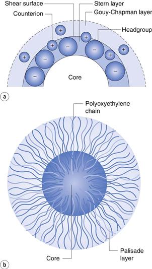
A typical micelle is a spherical or near-spherical structure composed of some 50–100 surfactant molecules. The radius of the micelle will be slightly less than that of the extended hydrocarbon chain (approximately 2.5 nm) with the interior core of the micelle having the properties of a liquid hydrocarbon. For ionic micelles, about 70–80% of the counter-ions will be attracted close to the micelle, thus reducing the overall charge. The compact layer around the core of an ionic micelle which contains the head groups and the bound counter-ions is called the Stern layer (see Fig. 5.13a). The outer surface of the Stern layer is the shear surface of the micelle. The core and the Stern layer together constitute what is termed the ‘kinetic micelle’. Surrounding the Stern layer is a diffuse layer called the Gouy–Chapman electrical double layer that contains the remaining counter-ions required to neutralize the charge on the kinetic micelle. The thickness of the double layer is dependent on the ionic strength of the solution and is greatly compressed in the presence of electrolyte. Non-ionic micelles have a hydrophobic core surrounded by a shell of oxyethylene chains which is often termed the palisade layer (Fig. 5.13b). As well as the water molecules that are hydrogen bonded to the oxyethylene chains, this layer is also capable of mechanically entrapping a considerable number of water molecules. Micelles of non-ionic surfactants tend, as a consequence, to be highly hydrated. The outer surface of the palisade layer forms the shear surface; that is, the hydrating molecules form part of the kinetic micelle.

Fig. 5.13 Schematic representation of (a) partial cross-section of an anionic micelle and (b) a non-ionic micelle.

Solubilization

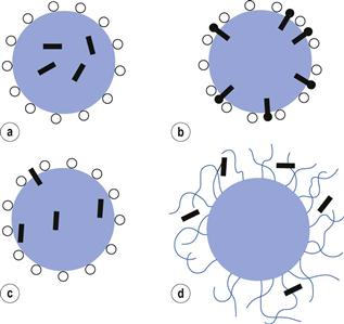
As outlined previously, the interior core of a micelle can be considered as having the properties of a liquid hydrocarbon and is thus capable of dissolving materials that are soluble in such liquids. This process, whereby water-insoluble or partly soluble substances are brought into aqueous solution by incorporation into micelles, is termed solubilization. The site of solubilization within the micelle is closely related to the chemical nature of the solubilizate. It is generally accepted that non-polar solubilizates (aliphatic hydrocarbons, for example) are dissolved in the hydrocarbon core (Fig. 5.14a). Water-insoluble compounds containing polar groups are orientated with the polar group at the surface of the ionic micelle amongst the micellar charged head groups, and the hydrophobic group buried inside the hydrocarbon core of the micelle (Fig. 5.14b). Slightly polar solubilizates without a distinct amphiphilic structure partition between the micelle surface and core (Fig. 5.14c). Solubilization in non-ionic polyoxyethylated surfactants can also occur in the polyoxyethylene shell (palisade layer) which surrounds the core (Fig. 5.14d); thus p-hydroxy benzoic acid is solubilized entirely within this region hydrogen bonded to the ethylene oxide groups, whilst esters such as the parabens are located at the shell core junction.

Fig. 5.14 Schematic representation of sites of solubilization in ionic and non-ionic micelles. (a) non-polar solubilizate; (b) amphipathic solubilizate; (c) slightly polar solubilizate; (d) polar solubilizate in polyoxyethylene shell of a non-ionic micelle.

The maximum amount of solubilizate that can be incorporated into a given system at a fixed concentration is termed the maximum additive concentration (MAC). The simplest method of determining the MAC is to prepare a series of vials containing surfactant solution of known concentration. Increasing concentrations of solubilizate are added and the vials are then sealed and agitated until equilibrium conditions are established. The maximum concentration of solubilizate forming a clear solution can be determined by visual inspection or from turbidity measurements on the solutions. Solubility data are expressed as a solubility versus concentration curve or as phase diagrams. The latter are preferable since a three-component phase diagram completely describes the effect of varying all three components of the system: namely, the solubilizate, the solubilizer and the solvent.

Pharmaceutical applications of solubilization

A wide range of insoluble drugs has been formulated using the principle of solubilization, some of which will be considered here.

Phenolic compounds such as cresol, chlorocresol, chloroxylenol and thymol are frequently solubilized with a soap to form clear solutions which are widely used for disinfection. Pharmacopoeial solutions of chloroxylenol, for example, contain 5% v/v chloroxylenol with terpineol in an alcoholic soap solution.

Non-ionic surfactants can be used to solubilize iodine; such iodine-surfactant systems (referred to as iodophors) are more stable than iodine–iodide systems. They are preferable in instrument sterilization since corrosion problems are reduced. Loss of iodine by sublimation from iodophor solutions is significantly less than from simple iodine solutions. There is also evidence of an ability of the iodophor solution to penetrate hair follicles of the skin, so enhancing the activity.

The low solubility of steroids in water presents a problem in their formulation for ophthalmic use. Because such formulations are required to be optically clear, it is not possible to use oily solutions or suspensions and there are many examples of the use of non-ionic surfactants as a means of producing clear solutions which are stable to sterilization. In most formulations, solubilization has been effected using polysorbates or polyoxyethylene sorbitan esters of fatty acids.

The polysorbate non-ionics have also been employed in the preparation of aqueous injections of the water-insoluble vitamins A, D, E and K.

Whilst solubilization is an excellent means of producing an aqueous solution of a water-insoluble drug, it should be realized that it may well have effects on the drug’s activity and absorption characteristics. As a generalization, it may be said that low concentrations of surface-active agents increase absorption, possibly due to enhanced contact of the drug with the absorbing membrane, whilst concentrations above the CMC either produce no additional effect or cause decreased absorption. In the latter case the drug may be held within the micelles so that the concentration available for absorption is reduced. For a wider appreciation of this topic, the review by Attwood & Florence (1983) can be consulted.

Solubilization and drug stability

Solubilization has been shown to have a modifying effect on the rate of hydrolysis of drugs. Non-polar compounds solubilized deep in the hydrocarbon core of a micelle are likely to be better protected against attack by hydrolysing species than more polar compounds located closer to the micellar surface. For example, the alkaline hydrolysis of benzocaine and homatropine in the presence of several non-ionic surfactants is retarded, the less polar benzocaine showing a greater increase in stability compared to homatropine because of its deeper penetration into the micelle. An important factor in considering the breakdown of a drug located close to the micellar surface is the ionic nature of the surface-active agent. For base-catalysed hydrolysis, anionic micelles should give an enhanced protection due to repulsion of the attacking OH⁻ group. For cationic micelles there should be the converse effect. Whilst this pattern has been found, enhanced protection by cationic micelles also occurs, suggesting that in these cases the positively charged polar head groups hold the OH⁻ groups and thus block their penetration into the micelle.

Protection from oxidative degradation has also been found with solubilized systems.

As indicated earlier, drugs may be surface active. Such drugs form micelles and this self-association has been found in some cases to increase the drug’s stability. Thus micellar solutions of penicillin G have been reported to be 2.5 times more stable than monomeric solutions under conditions of constant pH and ionic strength.

Detergency

Detergency is a complex process whereby surfactants are used for the removal of foreign matter from solid surfaces, be it removal of dirt from clothes or cleansing of body surfaces. The process includes many of the actions characteristic of specific surfactants. Thus, the surfactant must have good wetting characteristics so that the detergent can come into intimate contact with the surface to be cleaned. The detergent must have the ability to remove the dirt into the bulk of the liquid; the dirt/water and solid/water interfacial tensions are lowered and thus the work of adhesion between the dirt and solid is reduced, so that the dirt particle may be easily detached. Once removed, the surfactant can be adsorbed at the particle surface, creating charge and hydration barriers which prevent deposition. If the dirt is oily it may be emulsified or solubilized.

Coarse disperse systems

Suspensions

A pharmaceutical suspension is a coarse dispersion in which insoluble particles, generally greater than 1 µm in diameter, are dispersed in a liquid medium, usually aqueous.

An aqueous suspension is a useful formulation system for administering an insoluble or poorly soluble drug. The large surface area of dispersed drug ensures a high availability for dissolution and hence absorption. Aqueous suspensions may also be used for parenteral and ophthalmic use and provide a suitable form for the application of dermatological materials to the skin. Suspensions are used similarly in veterinary practice and a closely allied field is that of pest control. Pesticides are frequently presented as suspensions for use as fungicides, insecticides, ascaricides and herbicides.

An acceptable suspension possesses certain desirable qualities amongst which are the following: the suspended material should not settle too rapidly; the particles which do settle to the bottom of the container must not form a hard mass but should be readily dispersed into a uniform mixture when the container is shaken; and the suspension must not be too viscous to pour freely from the orifice of the bottle or to flow through a syringe needle.

Physical stability of a pharmaceutical suspension may be defined as the condition in which the particles do not aggregate and in which they remain uniformly distributed throughout the dispersion. Since this ideal situation is seldom realized, it is appropriate to add that if the particles do settle they should be easily resuspended by a moderate amount of agitation.

The major difference between a pharmaceutical suspension and a colloidal dispersion is one of size of dispersed particles, with the relatively large particles of a suspension liable to sedimentation due to gravitational forces. Apart from this, suspensions show most of the properties of colloidal systems. The reader is referred to Chapter 26 for an account of the formulation of suspensions.

Controlled flocculation

A suspension in which all the particles remain discrete would, in terms of the DLVO theory, be considered to be stable. However, with pharmaceutical suspensions, in which the solid particles are very much coarser, such a system would sediment because of the size of the particles. The electrical repulsive forces between the particles allow the particles to slip past one another to form a close packed arrangement at the bottom of the container, with the small particles filling the voids between the larger ones. The supernatant liquid may remain cloudy after sedimentation due to the presence of colloidal particles that will remain dispersed. Those particles lowermost in the sediment are gradually pressed together by the weight of the ones above. The repulsive barrier is thus overcome, allowing the particles to pack closely together. Physical bonding leading to ‘cake’ or ‘clay’ formation may then occur due to the formation of bridges between the particles resulting from crystal growth and hydration effects, forces greater than agitation usually being required to disperse the sediment. Coagulation in the primary minimum, resulting from a reduction in the zeta potential to a point where attractive forces predominate, thus produces coarse compact masses with a ‘curdled’ appearance, which may not be readily dispersed.

On the other hand, particles flocculated in the secondary minimum form a loosely bonded structure, called a flocculate or floc. A suspension consisting of particles in this state is said to be flocculated. Although sedimentation of flocculated suspensions is fairly rapid, a loosely packed, high-volume sediment is obtained in which the flocs retain their structure and the particles are easily resuspended. The supernatant liquid is clear because the colloidal particles are trapped within the flocs and sediment with them. Secondary minimum flocculation is therefore a desirable state for a pharmaceutical suspension.

Particles greater than 1 µm radius should, unless highly charged, show a sufficiently deep secondary minimum for flocculation to occur because the attractive force between particles, V_A, depends on particle size. Other contributing factors to secondary minimum flocculation are shape (asymmetric particles, especially those that are elongated, being more satisfactory than spherical ones) and concentration. The rate of flocculation depends on the number of particles present, so that the greater the number of particles, the more collisions there will be and flocculation is more likely to occur. However, it may be necessary, as with highly charged particles, to control the depth of the secondary minimum to induce a satisfactory flocculation state. This can be achieved by addition of electrolytes or ionic surface-active agents which reduce the zeta potential and hence V_R, resulting in the displacement of the whole of the DLVO plot to give a satisfactory secondary minimum, as indicated in Figure 5.5. The production of a satisfactory secondary minimum leading to floc formation in this manner is termed controlled flocculation.

A convenient parameter for assessing a suspension is the sedimentation volume ratio, F, which is defined as the ratio of the final settled volume V_u to the original volume V_o:

(5.28)

The ratio F gives a measure of the aggregated-deflocculated state of a suspension and may usefully be plotted, together with the measured zeta potential, against concentration of additive, enabling an assessment of the state of the dispersion to be made in terms of the DLVO theory. The appearance of the supernatant liquid should be noted and the redispersibility of the suspensions evaluated.

It should be pointed out that in using the controlled flocculation approach to suspension formulation, it is important to work at a constant, or narrow, pH range because the magnitude of the charge on the drug particle can vary greatly with pH.

Other additives such as flavouring agents may also affect particle charge.

Steric stabilization of suspensions

As described earlier in this chapter, colloidal particles may be stabilized against coagulation in the absence of a charge on the particles by the use of non-ionic polymeric material – the concept of steric stabilization or protective colloid action. This concept may be applied to pharmaceutical suspensions where naturally occurring gums such as tragacanth and synthetic materials like non-ionic surfactants and cellulose polymers may be used to produce satisfactory suspensions. These materials may increase the viscosity of the aqueous vehicle and thus slow the rate of sedimentation of the particles, but they will also form adsorbed layers around the particles so that the approach of their surfaces and aggregation to the coagulated state is hindered.

Repulsive forces arise as the adsorbed layers interpenetrate and, as explained above, these have an enthalpic component due to release of water of solvation from the polymer chains and an entropic component due to movement restriction. As a result, the particles will not usually approach one another closer than twice the thickness of the adsorbed layer.

However, as indicated above in the discussion on controlled flocculation, from a pharmaceutical point of view an easily dispersed aggregated system is desirable. To produce this state, a balance between attractive and repulsive forces is required. This is not achieved by all polymeric materials, and the equivalent of deflocculated and caked systems may be produced. The balance of forces appears to depend on both the thickness and the concentration of the polymer in the adsorbed layer. These parameters determine the Hamaker constant and hence the attractive force, which must be large enough to cause aggregation of the particles comparable to flocculation. The steric repulsive force, which depends on the concentration and degree of solvation of the polymer chains, must be of sufficient magnitude to prevent close approach of the uncoated particles, but low enough so that the attractive force is dominant, leading to aggregation at about twice the adsorbed layer thickness. It has been found, for example, that adsorbed layers of certain polyoxyethylene-polyoxypropylene block copolymers will product satisfactory flocculated systems, whilst many nonyl phenyl ethoxylates will not. With both types of surfactant, the molecular moieties producing steric repulsion are hydrated ethylene oxide chains, but the concentration of these in the adsorbed layers varies, giving the results indicated above.

Wetting problems

One of the problems encountered in dispersing solid materials in water is that the powder may not be readily wetted (explained in Chapter 4). This may be due to entrapped air or to the fact that the solid surface is hydrophobic. The wettability of a powder may be described in terms of the contact angle, θ, which the powder makes with the surface of the liquid. This is described by:

(as 4.1)

(5.29)

where γ_SV, γ_SL and γ_LV are the respective interfacial tensions.

For a liquid to completely wet a powder, there should be a decrease in the surface free energy as a result of the immersion process. Once the particle is submerged in the liquid, the process of spreading wetting becomes important. In most cases where water is involved, the reduction of contact angle may only be achieved by reducing the magnitude of γ_LV and γ_SL by the use of a wetting agent. The wetting agents are surfactants that not only reduce γ_LV but also adsorb on to the surface of the powder, thus reducing γ_SL. Both of these effects reduce the contact angle and improve the dispersibility of the powder.

Problems may arise because of the build-up of an adhering layer of suspension particles on the walls of the container just above the liquid line that occurs as the walls are repeatedly wetted by the suspension. This layer subsequently dries to form a hard, thick crust. Surfactants reduce this adsorption by coating both the container and particle surfaces such that they repel, reducing adsorption.

Rheological properties of suspensions

Flocculated suspensions tend to exhibit plastic or pseudoplastic flow, depending on concentration, while concentrated deflocculated dispersions tend to be dilatant (Chapter 6). This means that the apparent viscosity of flocculated suspensions is relatively high when the applied shearing stress is low, but it decreases as the applied stress increases and the attractive forces producing the flocculation are overcome. Conversely, the apparent viscosity of a concentrated deflocculated suspension is low at low shearing stress, but increases as the applied stress increases. This effect is due to the electrical repulsion that occurs when the charged particles are forced close together (see the DLVO plot of potential energy of interaction between particles; Fig. 5.4), causing the particles to rebound, creating voids into which the liquid flows, leaving other parts of the dispersion dry. In addition to the rheological problems associated with particle charge, the sedimentation behaviour is also of course influenced by the rheological properties of the liquid continuous phase.

Emulsions

An emulsion is a system consisting of two immiscible liquid phases, one of which is dispersed throughout the other in the form of fine droplets. A third component, the emulsifying agent, is necessary to stabilize the emulsion.

The phase that is present as fine droplets is called the disperse phase and the phase in which the droplets are suspended is the continuous phase. Most emulsions will have droplets with diameters of 0.1–100 µm and are inherently unstable systems; smaller globules exhibit colloidal behaviour and have the stability of a hydrophobic colloidal dispersion.

Pharmaceutical emulsions usually consist of water and an oil. Two main types of emulsion can exist, oil-in-water (o/w) and water-in-oil (w/o), depending upon whether the continuous phase is aqueous or oily. More complicated emulsion systems may exist; for example, an oil droplet enclosing a water droplet may be suspended in water to form a water-in-oil-in-water emulsion (w/o/w). Such systems, and their o/w/o counterparts, are termed multiple emulsions and are of interest as delayed-action drug delivery vehicles.

The pharmaceutical applications of emulsions as a dosage forms are discussed in Chapter 27. Traditionally, emulsions have been used to render oily substances such as castor oil in a more palatable form. It is possible to formulate together oil-soluble and water-soluble medicaments in emulsions, and drugs may be more easily absorbed owing to the finely divided condition of emulsified substances.

A large number of bases used for topical preparations are emulsions, water miscible being o/w type and greasy bases being w/o. The administration of oils and fats by intravenous infusion, as part of a total parenteral nutrition programme, has been made possible by the use of suitable non-toxic emulsifying agents like lecithin. Here, the control of particle size of emulsion droplets is of paramount importance in the prevention of the formation of emboli.

Microemulsions

Unlike the coarse emulsions described above, microemulsions are homogeneous, transparent systems that are thermodynamically stable. Moreover, they form spontaneously when the components are mixed in the appropriate ratios. They can be dispersions of oil in water or water in oil but the droplet size is very much smaller, 5–140 nm, than in coarse emulsions. They are essentially swollen micellar systems, but obviously the distinction between a micelle containing solubilized oil and an oil droplet surrounded by an interfacial layer largely composed of surfactant is difficult to assess.

An essential requirement for their formation and stability is the attainment of a very low interfacial tension. It is generally not possible to achieve the required lowering of interfacial tension with a single surfactant and it is necessary to include a second amphiphile, usually a medium chain length alcohol, in the formulation. The second amphiphile is referred to as the cosurfactant.

Although microemulsions have many advantages over coarse emulsions, particularly their transparency and stability, they require much larger amounts of surfactant for their formulation which restricts the choice of acceptable components.

Theory of emulsion stabilization

Interfacial films.

When two immiscible liquids, e.g. liquid paraffin and water, are shaken together a temporary emulsion will be formed. The subdivision of one of the phases into small globules results in a large increase in surface area and hence interfacial free energy of the system. The system is thus thermodynamically unstable which results, in the first place, in the dispersed phase being in the form of spherical droplets (the shape of minimum surface area for a given volume) and, secondly, in coalescence of these droplets, causing phase separation, the state of minimum surface free energy.

The adsorption of a surface-active agent at the globule interface will lower the o/w interfacial tension, the process of emulsification will be made easier and the stability may be enhanced. However, if a surface-active agent such as sodium dodecyl sulfate is used, the emulsion, on standing for a short while, will still separate out into its constituent phases. On the other hand, substances like acacia, which are only slightly surface active, produce stable emulsions. Acacia forms a strong viscous interfacial film around the globules and it is thought that the characteristics of the interfacial film are most important in considering the stability of emulsions.

Pioneering work on emulsion stability by Schulman & Cockbain showed that a mixture of an oil-soluble alcohol such as cholesterol and a surface-active agent such as sodium cetyl (hexadecyl) sulfate was able to form a stable complex condensed film at the oil/water interface. This film was of high viscosity, sufficiently flexible to permit distortion of the droplets, resisted rupture and gave an interfacial tension lower than that produced by either component alone. The emulsion produced was stable, the charge arising from the sodium cetyl sulfate contributing to the stability as described for lyophobic colloidal dispersions. For complex formation at the interface, the correct ‘shape’ of molecule is necessary. Thus Schulman & Cockbain found that sodium cetyl sulfate stabilized an emulsion of liquid paraffin when elaidyl alcohol (the trans isomer) was the oil-soluble component but not when the cis isomer, oleyl alcohol, was used.

In practice, the oil-soluble and water-soluble components are dissolved in the appropriate phases and on mixing the two phases, the complex is formed at the interface. Alternatively, an emulsifying wax may be used consisting of a blend of the two components. The wax is dispersed in the oil phase and the aqueous phase added at the same temperature. Examples of such mixtures are given in Table 5.4.

Table 5.4

Emulsifying waxes

Product	Oil-soluble component	Water-soluble component
Emulsifying wax (anionic)	Cetostearyl alcohol	Sodium lauryl (dodecyl) sulfate
Cetrimide emulsifying wax (cationic)	Cetostearyl alcohol	Cetrimide (hexadecyl trimethyl ammonium bromide)
Cetomacrogol emulsifying wax (non-ionic)	Cetostearyl alcohol	Cetomacrogol (polyoxyethylene monohexadecyl ether)

This principle is also applied with the non-ionic emulsifying agents. For example, mixtures of sorbitan monooleate and polyoxyethylene sorbitan esters (e.g. polysorbate 80) have good emulsifying properties. Non-ionic surfactants are widely used in the production of stable emulsions and have the advantage over ionic surfactants of being less toxic and less sensitive to electrolytes and pH variation. These emulsifying agents are not charged and there is no electrical repulsive force contributing to stability. It is likely, however, that these substances, and the cetomacrogol emulsifying wax included in Table 5.4, sterically stabilize the emulsions as discussed under suspensions.

Hydrophilic colloids as emulsion stabilizers.

A number of hydrophilic colloids are used as emulsifying agents in pharmaceutical science. These include proteins (gelatin, casein) and polysaccharides (acacia, cellulose derivatives and alginates). These materials, which generally exhibit little surface activity, adsorb at the oil/water interface and form multilayers. Such multilayers have viscoelastic properties, resist rupture and presumably form mechanical barriers to coalescence. However, some of these substances have chemical groups which ionize, e.g. acacia consists of salts of arabic acid, proteins contain both amino and carboxylic acid groupings, thus providing electrostatic repulsion as an additional barrier to coalescence. Most cellulose derivatives are not charged. However, there is evidence from studies on solid suspensions that these substances sterically stabilize and it would appear probable that there will be a similar effect with emulsions.

Solid particles in emulsion stabilization.

Emulsions may be stabilized by finely divided solid particles if they are preferentially wetted by one phase and possess sufficient adhesion for one another so that they form a film around the dispersed droplets.

Solid particles will remain at the interface as long as a stable contact angle, θ, is formed by the liquid/liquid interface and the solid surface. The particles must also be of sufficiently low mass for gravitational forces not to affect the equilibrium. If the solid is preferentially wetted by one of the phases, then more particles can be accommodated at the interface if the interface is convex towards that phase. In other words, the liquid whose contact angle (measured through the liquid) is less than 90° will form the continuous phase (see Fig. 5.15). Aluminium and magnesium hydroxides and clays such as bentonite are preferentially wetted by water and thus stabilize o/w emulsions, e.g. liquid paraffin and magnesium hydroxide emulsion. Carbon black and talc are more readily wetted by oils and stabilize w/o emulsions.

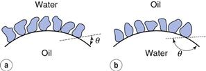
Fig. 5.15 Emulsion stabilization using solid particles. (a) Preferential wetting of solid by water, leading to an o/w emulsion. (b) Preferential wetting of solid by oil, leading to a w/o emulsion.

Emulsion type

When an oil, water and an emulsifying agent are shaken together, what decides whether an o/w or w/o emulsion will be produced? A number of simultaneous processes have to be considered, for example, droplet formation, aggregation and coalescence of droplets, and interfacial film formation. On shaking together oil and water, both phases initially form droplets. The phase that persists in droplet form for the longer time should become the disperse phase and it should be surrounded by the continuous phase formed from the more rapidly coalescing droplets. The phase volumes and interfacial tensions will determine the relative number of droplets produced and hence the probability of collision, i.e. the greater the number of droplets, the higher the chance of collision, so that the phase present in greater amount should finally become the continuous phase. However, emulsions containing well over 50% of disperse phase are common.

A more important consideration is the interfacial film produced by the adsorption of emulsifier at the o/w interface. Such films significantly alter the rates of coalescence by acting as physical and chemical barriers to coalescence. As indicated in the previous section, the barrier at the surface of an oil droplet may arise because of electrically charged groups producing repulsion between approaching droplets, or because of the steric repulsion, enthalpic in origin, from hydrated polymer chains. The greater the number of charged molecules present, or the greater the number of hydrated polymer chains at the interface, the greater will be the tendency to reduce oil droplet coalescence. On the other hand, the interfacial barrier for approaching water droplets arises primarily because of the non-polar or hydrocarbon portion of the interfacial film. The longer the hydrocarbon chain length and the greater the number of molecules present per unit area of film, the greater is the tendency for water droplets to be prevented from coalescing. Thus, it may be said generally that it is the dominance of the polar or non-polar characteristics of the emulsifying agent which plays a major part in the type of emulsion produced.

It would appear, then, that the type of emulsion formed, depending as it does on the polar/non-polar characteristics of the emulsifying agent, is a function of the relative solubility of the emulsifying agent, the phase in which it is more soluble being the continuous phase. This is a statement of what is termed the Bancroft rule, an empirical observation.

The foregoing helps to explain why charged surface-active agents such as sodium and potassium oleates which are highly ionized and possess strong polar groups favour o/w emulsions, whereas calcium and magnesium soaps which are little dissociated tend to produce w/o emulsions. Similarly, non-ionic sorbitan esters favour w/o emulsions whilst o/w emulsions are produced by the more hydrophilic polyoxyethylene sorbitan esters.

By reason of the stabilizing mechanism involved, polar groups are far better barriers to coalescence than their non-polar counterparts. It is thus possible to see why o/w emulsions can be made with greater than 50% disperse phase and w/o emulsions are limited in this respect and invert (change type) if the amount of water present is significant.

Hydrophile—lipophile balance.

The fact that a more hydrophilic interfacial barrier favours o/w emulsions whilst a more non-polar barrier favours w/o emulsions is employed in the hydrophile–lipophile balance (HLB) system for assessing surfactants and emulsifying agents, which was introduced by Griffin. Here an HLB number is assigned to an emulsifying agent that is characteristic of its relative polarity. Although originally conceived for non-ionic emulsifying agents with polyoxyethylene hydrophilic groups, it has since been applied with varying success to other surfactant groups, both ionic and non-ionic.

By means of this number system, an HLB range of optimum efficiency for each class of surfactant is established, as seen in Figure 5.16. This approach is empirical but it does allow comparison between different chemical types of emulsifying agent.

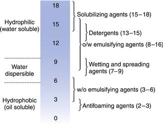
Fig. 5.16 HLB scale showing classification of surfactant function.

There are several formulae for calculating HLB values of non-ionic surfactants. We can estimate values for polysorbates (Tweens) and sorbitan esters (Spans) from:

(5.30)

where E is the percentage by weight of oxyethylene chains and P is the percentage by weight of polyhydric alcohol groups (glycerol or sorbitol) in the molecule. If the surfactant contains only polyoxyethylene as the hydrophilic group then we can use a simpler form of the equation:

(5.31)

Alternatively, we can calculate HLB values directly from the chemical formula using empirically determined group numbers. The formula is then:

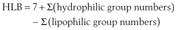(5.32)

Group numbers of some commonly occurring groups are given in Table 5.5. Finally, the HLB of polyhydric alcohol fatty acid esters such as glyceryl monostearate may be obtained from the saponification value, S, of the ester and the acid number, A, of the fatty acid using:

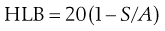(5.33)

In addition, it has been suggested that certain emulsifying agents of a given HLB value appear to work best with a particular oil phase and this has given rise to the concept of a required HLB value for any oil or combination of oils. However, this does not necessarily mean that every surfactant having the required HLB value will produce a good emulsion; specific surfactants may interact with the oil, with another component of the emulsion or even with each other.

Table 5.5

Group contributions to HLB values

Group	Contribution
SO₄Na	+38.7
COOK	+21.1
COONa	+19.1
SO₃Na	+11.0
N (tertiary amine)	+9.4
Ester (sorbitan ring)	+6.8
Ester (free)	+2.4
COOH	+2.1
OH (free)	+1.9
—O— (ether)	+1.3
OH (sorbitan)	+0.5
CH, CH₂ etc	0
OCH₂CH₂	+0.33
OCH(CH₃)CH₂	−0.15
(alkyl)	−0.475
CF₂, CF₃	−0.870

For reasons mentioned earlier, mixtures of surface-active agents give more stable emulsions than when used singly. The HLB of a mixture of surfactants, consisting of fraction x of A and (1 − x) of B, is assumed to be an algebraic mean of the two HLB numbers:

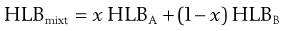(5.34)

It has been found that, at the optimum HLB for a particular emulsion, the mean particle size of the emulsion is at a minimum and this factor contributes to the stability of the emulsion system. The use of HLB values in the formulation of emulsions is discussed in Chapter 27.

Phase viscosity.

The emulsification process and the type of emulsion formed are influenced to some extent by the viscosity of the two phases. Viscosity can be expected to affect interfacial film formation because the migration of molecules of emulsifying agent to the oil/water interface is diffusion controlled. Droplet movement prior to coalescence is also affected by the viscosity of the medium in which the droplets are dispersed.

Stability of emulsions

A stable emulsion may be defined as a system in which the globules retain their initial character and remain uniformly distributed throughout the continuous phase. The function of the emulsifying agent is to form an interfacial film around the dispersed droplets; the physical nature of this barrier controls whether or not the droplets will coalesce as they approach one another. If the film is electrically charged, then repulsive forces will contribute to stability.

Separation of an emulsion into its constituent phases is termed cracking or breaking. It follows that any agent that will destroy the interfacial film will crack the emulsion. Some of the factors that cause an emulsion to crack are:

• the addition of a chemical that is incompatible with the emulsifying agent, thus destroying its emulsifying ability. Examples include surface-active agents of opposite ionic charge, e.g. the addition of cetrimide (cationic) to an emulsion stabilized with sodium oleate (anionic); addition of large ions of opposite charge, e.g. neomycin sulfate (cationic) to aqueous cream (anionic); addition of electrolytes such as calcium and magnesium salts to an emulsion stabilized with anionic surface-active agents

• bacterial growth – protein materials and non-ionic surface-active agents are excellent media for bacterial growth

• temperature change – protein emulsifying agents may be denatured and the solubility characteristics of non-ionic emulsifying agents change with a rise in temperature; heating above 70 °C destroys most emulsions. Freezing will also crack an emulsion; this may be because the ice formed disrupts the interfacial film around the droplets.

Other ways in which an emulsion may show instability are as follows.

Flocculation.

Even though a satisfactory interfacial film is present around the oil droplets, secondary minimum flocculation, as described earlier in this chapter under the discussion on the DLVO theory of colloid stability, is likely to occur with most pharmaceutical emulsions. The globules do not coalesce and may be redispersed by shaking. However, due to the closeness of approach of droplets in the floccule, if any weaknesses in the interfacial films occur then coalescence may follow. Flocculation should not be confused with creaming (see below). The former is due to the interaction of attractive and repulsive forces and the latter due to density differences in the two phases. Both may occur.

Phase inversion.

As indicated under the section on emulsion type, phase volume ratio is a contributory factor to the type of emulsion formed. Although it was stated there that stable emulsions containing more than 50% of disperse phase are common, attempts to incorporate excessive amounts of disperse phase may cause cracking of the emulsion or phase inversion (conversion of an o/w emulsion to w/o or vice versa). It can be shown that uniform spheres arranged in the closest packing will occupy 74% of the total volume irrespective of their size. Thus Ostwald suggested that an emulsion which resembles such an arrangement of spheres would have a maximum disperse phase concentration of the same order. Although it is possible to obtain more concentrated emulsions than this, because of the non-uniformity of size of the globules and the possibility of deformation of shape of the globules, there is a tendency for emulsions containing more than about 70% disperse phase to crack or invert.

Further, any additive that alters the HLB of an emulsifying agent may alter the emulsion type; thus addition of a magnesium salt to an emulsion stabilized with sodium oleate will cause the emulsion to crack or invert.

The addition of an electrolyte to anionic and cationic surfactants may suppress their ionization due to the common ion effect and thus a w/o emulsion may result even though normally an o/w emulsion would be produced. For example, pharmacopoeial White Liniment is formed from turpentine oil, ammonium oleate, ammonium chloride and water. With ammonium oleate as emulsifying agent, an o/w emulsion would be expected but the suppression of ionization of the ammonium oleate by the ammonium chloride (the common ion effect), and a relatively large volume of turpentine oil, produce a w/o emulsion.

Emulsions stabilized with non-ionic emulsifying agents such as the polysorbates may invert on heating. This is due to the breaking of the H-bonds responsible for the hydrophilic characteristics of the polysorbate; its HLB value is thus altered and the emulsion inverts.

Creaming.

Many emulsions cream on standing. The disperse phase, according to its density relative to that of the continuous phase, rises to the top or sinks to the bottom of the emulsion, forming a layer of more concentrated emulsion. The commonest example is milk, an o/w emulsion, with cream rising to the top of the emulsion.

As mentioned earlier, flocculation may occur as well as creaming but not necessarily so. Droplets of the creamed layer do not coalesce, as may be found by gentle shaking which redistributes the droplets throughout the continuous phase. Although not so serious an instability factor as cracking, creaming is undesirable from a pharmaceutical point of view because a creamed emulsion is inelegant in appearance, provides the possibility of inaccurate dosage and increases the likelihood of coalescence since the globules are close together in the cream.

Those factors which influence the rate of creaming are similar to those involved in the sedimentation rate of suspension particles and are indicated by Stokes’ Law (Eqn 5.8) as follows:

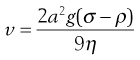(as 5.8)

where v is the velocity of creaming, a the globule radius, σ and ρ the densities of disperse phase and dispersion medium respectively, and η the viscosity of the dispersion medium. A consideration of this equation shows that the rate of creaming will be decreased by:

• a reduction in the globule size

• a decrease in the density difference between the two phases, and

• an increase in the viscosity of the continuous phase.

A decrease of creaming rate may therefore be achieved by homogenizing the emulsion to reduce the globule size and increasing the viscosity of the continuous phase, η by the use of thickening agents such as tragacanth or methylcellulose. It is seldom possible to satisfactorily adjust the densities of the two phases.

Assessment of emulsion stability.

Approximate assessments of the relative stabilities of a series of emulsions may be obtained from estimations of the degree of separation of the disperse phase as a distinct layer, or from the degree of creaming. Whilst separation of the emulsion into two layers, i.e. cracking, indicates gross instability, a stable emulsion may cream, creaming being simply due to density differences and easily reversed by shaking. Some coalescence may, however, take place due to the close proximity of the globules in the cream; similar problems occur with flocculation.

However, instability in an emulsion results from any process which causes a progressive increase in particle size and a broadening of the particle size distribution, so that eventually the dispersed particles become so large that they separate out as free liquid. Accordingly, a more precise method for assessing emulsion stability is to follow the globule size distribution with time. An emulsion approaching the unstable state is characterized by the appearance of large globules as a result of the coalescence of others.

Foams

A foam is a coarse dispersion of a gas in a liquid which is present as thin films or lamellae of colloidal dimensions between the gas bubbles.

Foams find application in pharmacy as aqueous and non-aqueous spray preparations for topical, rectal and vaginal medication and for burn dressings. Equally important, however, is the destruction of foams and the use of antifoaming agents. These are of importance in manufacturing processes, preventing foam in, for example, liquid preparations. In addition, foam inhibitors, such as the silicones, are used in the treatment of flatulence, for the elimination of gas, air or foam from the gastrointestinal tract prior to radiography and for the relief of abdominal distension and dyspepsia.

Due to their high interfacial area (and surface free energy), all foams are unstable in the thermodynamic sense. Their stability depends on two major factors: the tendency for the liquid films to drain and become thinner, and their tendency to rupture due to random disturbances such as vibration, heat and diffusion of gas from small bubbles to large bubbles. Gas diffuses from the small bubbles to the large because the pressure in the former is greater. This is a phenomenon of curved interfaces, the pressure difference, Δp being a function of the interfacial tension, γ, and the radius, r, of the droplet according to Δp = 2γ/r.

Pure liquids do not foam. Transient or unstable foams are obtained with solutes such as short chain acids and alcohols which are mildly surface active. However, persistent foams are formed by solutions of surfactants. The film in such foams consists of two monolayers of adsorbed surface-active molecules separated by an aqueous core. The surfactants stabilize the film by means of electrical double layer repulsion or steric stabilization as described for colloidal dispersions.

Foams are often troublesome and knowledge of the action of substances that cause their destruction is useful. There are two types of antifoaming agent:

• foam breakers such as ether and n-octanol. These substances are highly surface active and are thought to act by lowering the surface tension over small regions of the liquid film. These regions are rapidly pulled out by surrounding regions of higher tension, small areas of film are therefore thinned out and left without the properties to resist rupture

• foam inhibitors, such as polyamides and silicones. It is thought that these are adsorbed at the air/water interface in preference to the foaming agent, but they do not have the requisite ability to form a stable foam. They have a low interfacial tension in the pure state and may be effective by virtue of rapid adsorption.

Aerosols

Aerosols are colloidal dispersions of liquids or solids in gases. In general, mists and fogs possess liquid disperse phases whilst smoke is a dispersion of solid particles in gases. However, no sharp distinction can be made between the two kinds because liquid is often associated with the solid particles. A mist consists of fine droplets of liquid that may or may not contain dissolved or suspended material. If the concentration of droplets becomes high it may be called a fog.

While all the disperse systems mentioned above are less stable than colloids that have a liquid as dispersion medium, they have many properties in common with the latter and can be investigated in the same way. Particle size is usually within the colloidal range but if larger than 1 µm, the life of an aerosol is short because the particles settle out too quickly.

Preparation of aerosols

In common with other colloidal dispersions, aerosols may be prepared by either dispersion or condensation methods. The latter involve the initial production of supersaturated vapour of the material that is to be dispersed. This may be achieved by supercooling the vapour. The supersaturation eventually leads to the formation of nuclei, which grow into particles of colloidal dimensions. The preparation of aerosols by dispersion methods is of greater interest in pharmacy and may be achieved by the use of pressurized containers with, for example, liquefied gases used as propellants. If a solution or suspension of active ingredients is contained in the liquid propellant or in a mixture of this liquid and an additional solvent, then when the valve on the container is opened the vapour pressure of the propellant forces the mixture out of the container. The large expansion of the propellant at room temperature and atmospheric pressure produces a dispersion of the active ingredients in air. Although the particles in such dispersions are often larger than those in colloidal systems, these dispersions are still generally referred to as aerosols.

Application of aerosols in pharmacy

The use of aerosols as a dosage form is particularly important in the administration of drugs via the respiratory system. In addition to local effects, systemic effects may be obtained if the drug is absorbed into the blood stream from the lungs. Topical preparations (Chapter 39) are also well suited for presentation as aerosols. Therapeutic aerosols for inhalation are discussed in more detail in Chapter 37.

References

1. Attwood D, Florence AT. Surfactant Systems: Their Chemistry, Pharmacy and Biology. London: Chapman and Hall; 1983.

2. Shaw DJ. Introduction to Colloid and Surface Chemistry. 4th edn Oxford: Butterworth-Heinemann; 1992.

Bibliography

1. Florence AT, Attwood D. Physicochemical Principles of Pharmacy. 5th edn London: Pharmaceutical Press; 2011.

2. Rosen MJ. Surfactants and Interfacial Phenomena. 2nd edn New York: John Wiley; 1989.

Recent Posts

Meta

Categories

Search Engine

Disperse systems