Diffusion-Weighted Magnetic Resonance Imaging: Principles and Implementation in Clinical and Research Settings

Published on 27/02/2015 by admin

Filed under Pediatrics

Last modified 22/04/2025

Print this page

This article have been viewed 2554 times

Chapter 26

Diffusion-Weighted Magnetic Resonance Imaging

Principles and Implementation in Clinical and Research Settings

Jessica L. Wisnowski, Rafael C. Ceschin and Vincent J. Schmithorst

Of the advanced magnetic resonance imaging (MRI) modalities, diffusion-weighted (DW) MRI has probably garnered the most excitement in both clinical and research settings during the past decade. Standard now in nearly every neuroimaging MR protocol, DW-MRI has demonstrated substantial clinical utility in the detection of acute ischemia, the differential diagnosis of intracranial lesions, and the evaluation of white matter. More recently, DW-MRI, or more specifically, diffusion tensor imaging (DTI) and other high-angular resolution diffusion imaging (HARDI) models, have been applied to the evaluation of normal developmental processes and pathology, particularly that which involves the white matter. Numerous postprocessing methods have been developed that not only allow for group level comparisons of the underlying “tissue microstructure” but also allow for estimation (and visual representation) of the underlying white matter “tracts.” In this chapter, we will (1) review the underlying principles of DW-MRI acquisitions; (2) review basic diffusion-weighted imaging (DWI) acquisitions (DWI and its application in clinical settings); (3) review DTI models and postprocessing methods, with emphasis on the strengths and potential pitfalls in both clinical and research settings; and (4) review advanced diffusion imaging models (e.g., diffusion kurtosis imaging [DKI], HARDI, Q-ball, and diffusion spectrum imaging [DSI]). Further examples of the application of DW-MRI will be evident in numerous other chapters in this volume.

Underlying Principles of DW-MRI Acquisition

At its core, DW-MRI involves the application of two additional pulses of magnetic field gradient (called “diffusion-encoding” or “diffusion-sensitizing” gradients) to a T2-weighted sequence after the excitation pulse but before the readout. During the first gradient pulse, spin precession is accelerated in accordance with the spatial position of the individual water molecules; spins associated with water molecules with a high Z coordinate, for example, will precess more quickly after administration of a gradient pulse along the Z direction, whereas spins associated with water molecules with a low Z coordinate will precess more slowly. Therefore the net effect of the first gradient pulse on the ensemble of spins is that the spins begin precessing at different rates and consequently “dephase,” resulting in signal attenuation. The second gradient pulse is equal in direction, magnitude, and duration (δ) to the first and is either of opposite polarity (in the case of a gradient echo acquisition) or of the same polarity (in the case of a spin echo acquisition) but placed after a 180-degree refocusing pulse. Assuming that the spins do not move from their original locations, the effect of the second gradient pulse will be to precisely undo the effect of the first and thus “rephase” the spins so there is no longer any signal attenuation due to spin dephasing. However, under physiologic conditions, water molecules possess thermal energy and therefore will move a finite distance away from their original locations during the time between gradient pulses (Δ). Thus the rephasing is incomplete and the signal will be attenuated compared with the signal with no diffusion-sensitizing gradients.

Assuming that the movement of water molecules is not hindered by any form of barrier (so-called “free diffusion”), the mean squared distance that the spins will move over a given period is described by the Einstein-Smoluchowsky equation and is linearly proportional to the time (Δ) and to the self-diffusion coefficient D. The amount of attenuation is a function of the gradient strength G, gradient duration δ, time between gradient pulses Δ, and diffusion coefficient D. Typically G, δ, and Δ are combined to derive the “b-value”; the higher the b-value, the greater the signal attenuation in the resultant DW images (Fig. 26-1). In fact, signal attenuation is exponential, where S is the measured signal and S₀ is the signal in the absence of diffusion weighting. As a result, D (measured in mm²/s) can be estimated by obtaining DW images at different b-values or by obtaining images with and without diffusion weighting.

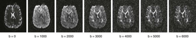
Figure 26-1 Changing b-value.
Displayed are corresponding slices from a single subject imaged at multiple b-values. Notice how contrast between gray and white matter increases with the increasing b-value, whereas overall signal/noise ratio decreases. (Data courtesy Justin Haldar, University of Southern California, Department of Electrical Engineering.)

However, the diffusion of water molecules in the brain differs in two important respects from free diffusion. First, the diffusion of water is hindered by a variety of barriers, including axon sheaths and glial cell and astrocyte membranes. Hence the measured diffusion coefficient is not a self-diffusion coefficient and therefore is referred to as an apparent diffusion coefficient (ADC). Furthermore, the diffusion of water in the brain is not isotropic (i.e., independent of direction). For instance, diffusivity along an axon direction will be larger than diffusivity perpendicular to the axon direction. Hence DW images often are obtained using a variety of gradient directions to infer information about the diffusivity of water molecules in different directions; the amount of attenuation in the DW images is dependent on the diffusion of water molecules only in the direction of the applied diffusion-encoding gradients.

It also is important to note that because DW measurements reflect an attenuation of signal at a given spatial location, maintenance of sufficient signal to noise in the resultant data is an inherent challenge in DWI. Moreover, the time needed to acquire data sufficient for some of the most advanced postprocessing techniques, which require acquisitions at many different gradient direction and b-values, is often well outside of what is typically feasible in clinical settings and in many pediatric populations. Thus in practice, most pediatric DW-MRI studies generally are limited to the more basic DW-MRI models (i.e., DTI, described in a later section of this chapter), although recent developments provide hope that other DW-MRI techniques soon will be clinically feasible.

Diffusion Weighting, Apparent Diffusivity, and Their Application in Clinical Settings

Clinically relevant information is available even from a single DWI acquisition. For instance, diffusion is restricted in regions of cytotoxic edema after a stroke, and these regions therefore will be hyperintense on DW images. However, typical DWI acquisitions are strongly T2-weighted, because a long echo time is necessary as a result of the time needed to apply the diffusion-sensitizing gradients. Therefore it is important to distinguish hyperintensity on DWI that represents true diffusion restriction from hyperintensity that reflects tissue T2 prolongation (often termed “T2 shine-through”). This differentiation usually is performed by the additional acquisition of an image without diffusion weighting (e.g., b = 0) and quantifying ADC on a pixel-by-pixel basis, which subsequently can be represented in gray scale as an ADC map. Additionally, instead of a single DW acquisition, three DW images typically are acquired using three orthogonal gradient directions, and the results are averaged to obtain directionally averaged DW images and ADC maps to minimize the effects of anisotropy. The directionally averaged ADC map is proportional to the trace of the diffusion tensor (described later), and thus the DWI images and ADC maps often are referred to as “trace-weighted DWI” and “trace diffusion tensor maps,” respectively (Fig. 26-2).

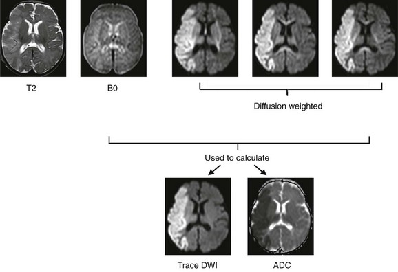
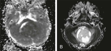
Figure 26-2 Diffusion-weighted (DW) imaging demonstrated in a 3-week-old neonate with an acute stroke.
Top row, Corresponding slices from an axial T2-weighted and DW-magnetic resonance imaging scan. In most protocols, three diffusion-encoding directions (rather than one) are acquired, averaged, and compared with the image without diffusion encoding (B0) to generate (bottom row) trace-weighted and apparent diffusivity maps that demonstrate areas of restricted diffusion as areas of high and low signal, respectively. Note that areas of directional anisotropy are visualized in each of the diffusion-encoding directions, but as a result of averaging, these areas are not apparent in the trace-weighted and apparent diffusion coefficient (ADC) maps.

As previously noted, in the past two decades, trace DW images with corresponding ADC values have demonstrated remarkable clinical utility in the detection of acute cerebral ischemia, often before such injuries otherwise become apparent. In persons with ischemia, a critical drop in cerebral blood perfusion leads to energy failure, and more specifically, a failure of the Na+/K+–adenosine triphosphatase pumps in the cell membrane. This phenomenon, in turn, leads to an influx of sodium (and other ions) and water into the cell, causing the cell to swell (i.e., cytotoxic edema). Although other events also might contribute to the change in ADC, it has been suggested that ADC is most sensitive to a small change in the distribution of water between extracellular and intracellular environments, and thus ADC can be viewed as a marker of fluid-electrolyte homeostasis.

In addition to fluid homeostasis and intracellular water, DWI and ADC also are sensitive to the relative properties of water in the extracellular space. Thus DWI also is useful in the differential diagnosis of intracranial lesions. In lesions with high cellularity (e.g., high-grade tumors), the increased cellularity restricts water motion in the extracellular space, resulting in decreased ADC in the lesion (or in areas of the lesion with relatively higher cellularity). Accordingly, DWI often can distinguish high-grade tumors such as primitive neuroectodermal tumors from other lower grade pediatric brain tumors such as ependymomas or astrocytomas (Fig. 26-3).

Figure 26-3 Apparent diffusion coefficient (ADC) and intracranial lesions.
A, The ADC map demonstrates restricted diffusion in a tumor with high cellularity (a medulloblastoma). B, The ADC map demonstrates increased diffusion in a tumor with low cellularity (a pilocytic astrocytoma).

Diffusion Tensor Imaging

Although three diffusion-sensitizing gradients are sufficient for calculating a directionally averaged ADC image, a minimum of six directions is needed to characterize diffusion anisotropy. Anisotropic diffusion is directionally dependent, as within white matter fiber bundles, and is distinguishable from isotropic diffusion, which is observed in free fluids (e.g., the lateral ventricles) (Fig. 26-4).

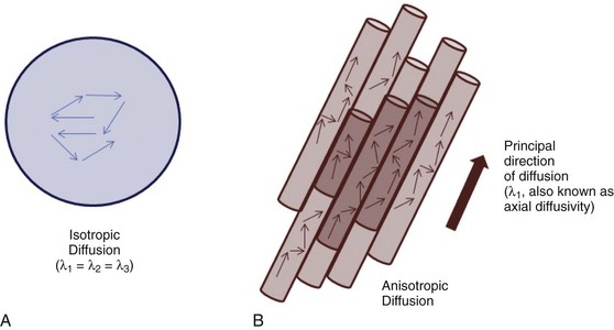
Figure 26-4 Isotropic and anisotropic diffusion.
A, Isotropic diffusion is exemplified by free diffusion such as in a large glass of water. B, Anisotropic diffusion occurs when diffusion is greater in one direction compared with the others, such as in axons. By convention, the principal eigenvalue (λ₁) represents diffusion along the preferred axis.

To calculate anisotropy, DTI models diffusion as a tensor quantity (a 3 × 3 matrix) on a voxel-by-voxel basis. Typically, the matrix is rotated such that anisotropy may be described in terms of three coordinate axes (“eigenvectors”), with the principal axis (the one corresponding to the largest “eigenvalue” λ₁, also known as λ, or axial diffusivity) being along the axis of preferred diffusion and the remaining two eigenvalues (λ₂ and λ₃) corresponding to vectors perpendicular to the principal axis. Eigenvalues λ₂ and λ₃ often are combined (averaged) to generate another metric referred to as radial diffusivity (λ). Importantly, although the 3 × 3 diffusion tensor may be ideal for estimating diffusion in a three-dimensional (3D) structure characterized by fiber bundles aligned in a single orientation, this model falls short if the underlying structure includes fiber bundles of different orientations (e.g., “crossing fibers”). Accordingly, potential pitfalls associated with DTI will be discussed in further detail later.

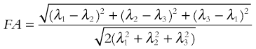
The most common anisotropy metric derived from DTI data is fractional anisotropy (FA). FA is a scalar metric (rather than a vector) and represents the degree of anisotropy at a given voxel. It is calculated by comparing the estimated diffusion along each of the three eigenvalues in accordance with the following equation:

As can be determined from this equation, FA can range from 0 (when λ₁ = λ₂ = λ₃, i.e., isotropic diffusion) to 1 (when λ₂ = λ₃ = 0, i.e., fully anisotropic). In adults, typical white-matter values range between 0.9 and 0.4 depending on whether the measurement is obtained in a region where fiber bundles are heavily myelinated, tightly packed, and uniformly oriented (e.g., in the corpus callosum) or in a region where the organization deviates from that (such as in the vicinity of crossing fibers), respectively. FA values are much lower in neonates (ranging between 0.45 and 0.1) but rapidly increase toward the adult range in the first 2 years of life and then continue to increase at a much lower rate through adolescence into adulthood.1–3

Because of the higher water content in the neonatal brain and the fact that this increase in extracellular water is associated with increased diffusivity and increased signal attenuation in the setting of diffusion encoding gradients, neonates often undergo imaging at a lower b-value (e.g., b = 700 s/mm²).

To further enhance the clinical utility of FA, FA often is combined with information regarding the direction of the principal eigenvector, yielding a color FA map (Fig. 26-5). The typical convention is to color pixels red when the principal eigenvector is in the left-right direction relative to the 3D coordinate space, green when the principal eigenvector is anterior-posterior, and blue when the principal eigenvector is inferior-superior.

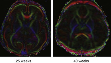
Figure 26-5 Color fractional anisotropy maps reconstructed from diffusion tensor imaging data acquired from a preterm neonate at 25 weeks and a term neonate at 40 weeks.
By convention, voxels in which the principal eigenvector (λ₁) is in a left-right orientation (relative to the slice) are colored in red, voxels in which λ₁ is in an anterior-posterior orientation are colored green, and voxels in which λ₁ is in a superior-inferior orientation are colored blue. Note the presence of high anisotropy in the cortex of the neonate at 25 weeks and that, by term, the cortex has lower anisotropy than the adjacent white matter.

Microstructural Integrity

The sensitivity of DTI to local (“microstructural”) tissue properties has rendered the technique a popular instrument for investigating the neuroanatomic underpinnings of various conditions (e.g., traumatic brain injury, multiple sclerosis, white matter injury of prematurity, autism, and dyslexia, but also such areas as normal development, learning, and musical training) at the level of gray and white matter tissue microstructure. Moreover, DTI sequences are readily available in most commercial MRI scanners, with the acquisition time necessary for a typical 30 to 60 direction DTI sequence being between 5 minutes to less than 15 minutes. Accordingly, DTI is not only feasible in most pediatric patients but also is a potential key to understanding the neuroanatomic basis for a wide range of conditions, many of which are not associated with visible changes on conventional T1- and T2-weighted imaging.

However, the precise interpretation for many of the differences in DTI measures of microstructure remains to be determined. Pioneering laboratory work by Sheng-Kwei Song and colleagues in mouse models demonstrated that myelin loss alone (without loss or degeneration of axons) results in an increase in radial diffusivity (RD), leaving axial diffusivity (AD) unchanged.⁴ In contrast, direct axonal damage results in a decrease in AD.⁵ Based on these findings, many researchers have drawn inverse conclusions on their own data—namely, that an increase in RD in a given white matter region reflects primarily damage to myelin, whereas a decrease in AD reflects primarily damage to axons. Unfortunately, the inverse conclusion is not necessarily valid. First, most of the laboratory work supporting the interpretation of AD and RD in relation to axonal pathology versus myelin has been carried out in the optic nerve, spinal cord, or corpus callosum.^4–6 These structures are unique in the central nervous system in that they contain fiber bundles essentially aligned along a single axis. In contrast, the cerebrum and even the brainstem have far fewer regions where the fiber bundles are organized along a single axis (it has been estimated that as many as 90% of white matter voxels in the cerebrum contain crossing fibers).⁷ It is not known how altering myelination or axonal integrity along a single fiber bundle, in the setting of multiple crossing fibers, would alter AD or RD. Accordingly, in the cerebrum, given available knowledge at this point, a more appropriate interpretation may be “altered microstructure,” with more specific conclusions being drawn from collateral information. However, this technique continues to show great promise.

Tractography

Some of the increasingly common—and most important—questions that researchers and neuroradiologists have aimed to address with use of DTI concerns anatomic connectivity (e.g., “Which cortical and subcortical regions are connected, and by which fiber pathways?” “How strong are the connections between X and Y? … in this population compared with that one?”). To address these types of questions, most researchers and clinicians begin by constructing a visual representation of the white matter fibers (or tracts). This task is carried out with use of computer algorithms that regard fiber tracts as a continuous trajectory derived from local (voxel or pixel) estimates of fiber orientation (e.g., eigenvectors; Fig. 26-6). This technique is commonly known as tractography. It should be emphasized that no tractography method is capable of reconstructing axonal fibers or even fiber bundles. Rather, these methods compute trajectories or pathways represented by the data, which, it is hoped, parallel the predominant trajectories of the underlying axonal fiber bundles.

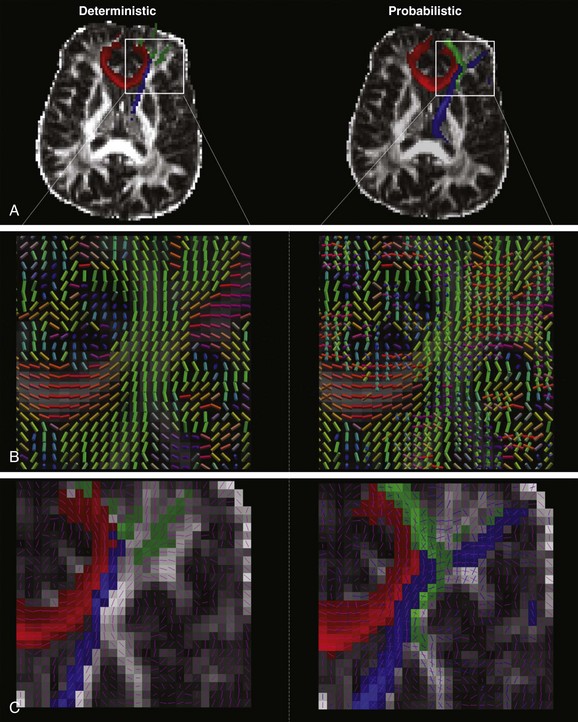
Figure 26-6 Deterministic and probabilistic tractography.
A, The same seed and waypoints were used to track anterior thalamic radiation (blue), genu of corpus callosum (red), and inferior frontooccipital fasciculus using deterministic (left) and probabilistic (right) algorithms on the same dataset acquired on a single subject. B, In deterministic tractography, the direction of anisotropy is considered to be along the axis of a single, principal eigenvector, which is represented voxelwise in the image on the left. (Color convention is as described in Fig. 26-5.) In contrast, probabilistic tractography models anisotropy as a probability distribution and allows for a two-fiber solution, which is represented on the right, with the major axis being larger in scale compared with the minor axis. C, The difference in output is clearly visualized in the region of the crossing fibers where, on the left, deterministic tractography (principal eigenvector overlaid as pink lines) fails to yield as many tracks as the output from the probabilistic algorithm on the right (again, principal and secondary eigenvectors are overlaid in pink and blue, respectively).

One of the most commonly used algorithms for tractography is known as fiber assignment by continuous tracking (also known as deterministic tractography).⁸ This algorithm proceeds from an initially determined point (seed region) and propagates pixel by pixel in the direction of the principal eigenvector until a predetermined lower FA threshold or maximal turning angle is reached, at which point the fiber path is terminated (see Fig. 26-6). The result is a streamline, a visual representation of anisotropic diffusion, and importantly, not an actual visual representation of axons or fiber bundles. Moreover, the number of streamlines originating from a particular seed region is directly proportional to the number of seed points within a given voxel, and accordingly, not directly related to the underlying anatomic connectivity. However, assuming the same number of seed points per given voxel are used across populations of interest (which, in most software packages, is not a number that can be manipulated by the operator), the number of streamlines can be considered a proxy for the underlying tissue microstructure, and accordingly, may be used as a metric in group-level comparisons.

One of the key limitations in tractography is that the mathematical model used to reconstruct DTI data assumes that a single fiber population exists in each voxel. However, at the resolution of a typical DTI acquisition (≥2 mm in each dimension), many voxels contain populations of fibers that are oriented in some manner other than parallel (from one third to 90%),7,8 including fibers that are crossing, fanning, branching, or bottlenecking. This crossing fiber problem is a significant concern if one is trying to carry out tractography on DTI data. First, the main effect of crossing or other nonparallel fiber orientations on the principal eigenvectors is to decrease the principal eigenvalue. This effect, in turn, results in a decrease in FA, which can cause tractography algorithms to prematurely stop if the FA value has fallen below the predetermined threshold. Second, because the algorithm follows only the principal eigenvector, it may generate spurious streamlines (e.g., a streamline that propagates into a crossing region perpendicular to the principal eigenvector could be made to bend and then continue in the new direction).

One method to address limitations associated with using deterministic tractography and DTI parameters is to use the information derived from the diffusion tensor fit to generate a 3D probability distribution regarding the diffusion of water molecules instead of constraining the molecules to only move along the direction of the principal eigenvector. In this way, probabilistic tractography algorithms allow water molecules to follow more than one orientation when passing through a voxel in a crossing region. Current probabilistic algorithms allow for the modeling of uncertainty of two (or more) fiber directions at each voxel. Tracking is done by launching a high number of streamlines from a seed region, and at each voxel—instead of deterministically following the principal eigenvector—drawing from the previously determined 3D probability distribution to propagate the tracts. Coherent fiber orientation is preserved by following the sampled direction that is most closely parallel to the previous location’s direction, as opposed to only following an arbitrary angle threshold. After a sufficient number of samples, the output is a probabilistic mapping of the uncertainty of fiber tracts at each voxel, with the dominant streamline surfacing as most probable (see Fig. 26-6). Notably, this method does not resolve the crossing-fiber problem with 100% certainty, but the resulting probabilistic map yields a much more robust estimate of the dominant fiber path when compared with deterministic approaches.⁹ Moreover, it also shows improvements in the rendering of the lateral corticospinal and corticobulbar tracts and the medial portion of the superior longitudinal fasciculus, which typically are not visualized by deterministic tractography. Figure 26-6 shows the comparison between deterministic and probabilistic algorithms in modeling fibers passing through a densely packed, high-fiber–crossing region of the brain. The probabilistic output shows significant improvement in delineating crossing fiber tracts, such as the inferior frontooccipital fasciculus and anterior thalamic radiation. Similar performance is noted in a single direction tract, as in the genu of the corpus callosum. Despite improved performance in modeling regions with crossing fiber tracts, probabilistic tractography still cannot completely overcome the limitation that the diffusion tensor model is not an adequate model for the underlying physiology in crossing fiber regions. This limitation requires more advanced approaches, as described in the next section.

Advanced Diffusion Imaging Techniques

Advanced diffusion imaging techniques have been proposed to address the two major limitations of the DTI model: multiple/crossing fiber bundles and signal attenuation that deviates from an exponential decay with increasing b-value. Currently these approaches have found limited clinical use because of their greater acquisition time and the greater computational resources needed for data analysis. However, as technology continues to improve, such techniques likely will become available for clinicians on clinical MRI scanners.

To address the problem of crossing fibers, HARDI methods (sometimes called “Q-ball”)10,11 sample a much larger number of diffusion directions (e.g., 64 to 256) and then typical DTI acquisitions (e.g., ~30, although DTI analysis is possible with as few as 6). Thus more complicated models than a simple tensor may be used to model the physiology (for further detail, the interested reader is referred to references 11 to 14 for an introduction).^12–15 It is possible, with these techniques, to model two, three, or even more crossing fiber bundles. In conjunction with probabilistic tractography, this provides a very powerful technique to model brain structural connectivity, and success has been seen even in regions with a very high number of crossing fibers. Typically, higher b-values are used in HARDI acquisitions (~3000 s/mm²) as opposed to those used in DTI (~1000 s/mm²). The reason is that diffusion is more restricted in directions perpendicular to the axon for intraaxonal water molecules, as opposed to interstitial water molecules, because the distance to the axonal membrane is smaller. Therefore the use of a higher b-value will suppress the signal from interstitial water, leading to a “cleaner” profile of fiber directionality.

Because most voxels consist of a mix of interstitial and intraaxonal water, the signal attenuation will deviate from an exponential decay with respect to b-value at higher b-values as the relative contribution from each type of water molecule changes. One approach to quantifying this deviation is DKI, which involves acquisition of data at several b-values; the “kurtosis” quantities describe deviations from exponential decay. (For details about DKI acquisition and analysis, see reference 16.) Compared with DTI, DKI has been shown to be more sensitive to subtle tissue microstructural changes¹⁷ and also has been found to yield additional information regarding pathologic changes in neural tissue, such as glioma grade discrimination.¹⁸ In typical DKI acquisitions, however, the angular resolution is not as great as HARDI because acquiring data at additional b-values is performed in lieu of additional diffusion gradient directions.

Finally, the “ultimate” in DWI acquisition is when acquisitions are obtained both at multiple gradient directions and multiple b-values,¹⁹ which will make possible a completely accurate specification of the water diffusion profiles, enabling the simultaneous modeling of crossing fiber bundles as well as nonexponential decay. This technique is called DSI or Q-space imaging. The acquisition demands are intense; a typical DSI protocol involves 512 separate DWI acquisitions, making the total acquisition time longer than 1 hour for typical DWI acquisition protocols.

Key Points

The diffusion of water is hindered by a variety of barriers, including axon sheaths and glial cell and astrocyte membranes.

The amount of attenuation in the DW images is dependent on the diffusion of water molecules only in the direction of the applied diffusion-encoding gradients.

In addition to fluid homeostasis and intracellular water, DWI and ADC also are sensitive to the relative properties of water in the extracellular space.

Because of the higher water content in the neonatal brain and because of the fact that this increase in extracellular water is associated with increased diffusivity and increased signal attenuation in the setting of diffusion encoding gradients, neonates often undergo imaging at a lower b-value (e.g., b = 700 s/mm²).

Tractography methods compute trajectories or pathways represented by the data, which, it is hoped, parallel the predominant trajectories of the underlying axonal fiber bundles.

Advanced diffusion imaging techniques address the two major limitations of conventional tractography: (1) multiple/crossing fiber bundles and signal attenuation that deviates from an exponential decay with increasing b-value.

References

1. Schmithorst, VJ, Wilke, M, Dardzinski, BJ, et al. Correlation of white matter diffusivity and anisotropy with age during childhood and adolescence: a cross-sectional diffusion-tensor MR imaging study. Radiology. 2002;222:212–218.
2. Schneider, JFL, Il’yasov, KA, Hennig, J, et al. Fast quantitative diffusion-tensor imaging of cerebral white matter from the neonatal period to adolescence. Neuroradiology. 2004;46:258–266.
3. Gao, W, Lin, G, Chen, Y, et al. Temporal and spatial development of axonal maturation and myelination of white matter in the developing brain. Am J Neuroradiol. 2009;30:290–296.
4. Song, S-K, Sun, S-W, Ramsbottom, MJ, et al. Dysmyelination revealed through MRI as increased radial (but unchanged axial) diffusion of water. Neuroimage. 2002;17(3):1429–1436.
5. Song, S-K, Sun, S-W, Ju, W-K, et al. Diffusion tensor imaging detects and differentiates axon and myelin degeneration in mouse optic nerve after retinal ischemia. Neuroimage. 2003;20:1714–1722.
6. Kim, JH, Loy, DN, Liang, H-F, et al. Noninvasive diffusion tensor imaging of evolving white matter pathology in a mouse model of acute spinal cord injury. Magn Reson Med. 2007;58:253–260.
7. Jeurissen, B, Leemans, A, Tournier, J-D, et al. Investigating the prevalence of complex fiber configurations in white matter tissue with diffusion magnetic resonance imaging. Hum Brain Mapp. 2012. [doi: 10.1002/hbm.22099 [E-pub ahead of print]].
8. Behrens, TEJ, Johansen-Berg, HJ, Jbabdi, S, et al. Probabilistic diffusion tractography with multiple fibre orientations: What can we gain? Neuroimage. 2007;34(1):144–155.
9. Mori, S, van Zijl, PCM. Fiber tracking: principles and strategies—a technical review. NMR Biomed. 2002;15:468–480.
10. Hirsch, JG, Schwenk, SM, Rossmanith, C, et al. Deviations from the diffusion tensor model as revealed by contour plot visualization using high angular resolution diffusion-weighted imaging (HARDI). MAGMA. 2003;16(2):93–102.
11. Tuch, DS. Q-ball imaging. Magn Reson Med. 2004;52(6):1358–1372.
12. Hess, CP, Mukherjee, P, Han, ET, et al. Q-ball reconstruction of multimodal fiber orientations using the spherical harmonic basis. Magn Reson Med. 2006;56(1):104–117.
13. Minati, L, Banasik, T, Brzezinski, J, et al. Elevating tensor rank increases anisotropy in brain areas associated with intra-voxel orientational heterogeneity (IVOH): a generalised DTI (GDTI) study. NMR Biomed. 2008;21(1):2–14.
14. Ozarslan, E, Shepherd, TM, Vemuri, BC, et al. Fast orientation mapping from HARDI. Med Image Comput Assist Interv. 2005;8(pt 1):156–163.
15. Ying, LL, Zou, YM, Klemer, DP, et al. Determination of fiber orientation in MRI diffusion tensor imaging based on higher-order tensor decomposition. Conf Proc IEEE Eng Med Biol Soc. 2007;2007:2065–2068.
16. Jensen, JH, Helpern, JA, Ramani, A, et al. Diffusional kurtosis imaging: the quantification of non-gaussian water diffusion by means of magnetic resonance imaging. Magn Reson Med. 2005;53(6):1432–1440.
17. Cheung, MM, Hui, ES, Chan, KC, et al. Does diffusion kurtosis imaging lead to better neural tissue characterization? A rodent brain maturation study. Neuroimage. 2009;45(2):386–392.
18. Raab, P, Hattingen, E, Franz, K, et al. Cerebral gliomas: diffusional kurtosis imaging analysis of microstructural differences. Radiology. 2010;254(3):876–881.
19. Basser, PJ. Relationships between diffusion tensor and q-space MRI. Magn Reson Med. 2002;47(2):392–397.