CHAPTER 17 Computed Tomography and Magnetic Resonance Imaging of the Brain
Computed Tomography of the Brain
History and Fundamentals
Computed tomography (CT), also called computed axial tomography (CAT), was developed in the early 1970s by Sir Geoffrey Hounsfield and his colleagues in England.1 It was possibly the single most important advance in medical imaging since the discovery of x-rays by Professor Wilhelm Roentgen. It represented the first commercially available imaging equipment that used the emerging technologic advances in computing to generate digital images displayed in gray scale. Its development revolutionized the evaluation of patients with neurological diseases and allowed noninvasive visualization of the inner body, which led to important diagnoses of diseases and abnormalities and played a key role in the diagnosis, management, and treatment of patients on a daily basis in the practice of medicine all over the world.2 Although its place in imaging of the brain and spine have been somewhat supplanted by another revolutionary technology known as magnetic resonance imaging (MRI), CT remains a workhorse and important first study of choice in many aspects of neurosurgery. Furthermore, important advances in CT technology during the past decade, such as multidetector configurations in newer CT scanners and ever increasing speed of computer technology that now allow very fast CT scanning of a patient in seconds rather than minutes, have resulted in a strong resurgence in its use. Such advances have led to the development of CT angiography (CTA) and perfusion CT (pCT), which have become important in noninvasive evaluation of cerebrovascular diseases. In addition, portable CT scanners can now provide high-quality images for point-of-care imaging in an intensive care unit setting and thereby avoid potential risks associated with transport of critically patients.
CT can be performed in various planes that depend on patient position and the CT gantry angle within its limited arc. For example, direct coronal-plane CT imaging of the paranasal sinuses or brain can be performed with the patient in a supine, “hanging-head” position with the head of the patient literally hanging over the edge of the CT scanner table or with the patient in the prone position and the neck hyperextended. However, most commonly, CT imaging of the brain and spine is performed in the axial plane with the patient in a supine position on the scanner table and the head and neck in a neutral position. The need for a direct coronal patient position is less important since the advent of high-resolution multiplanar reconstruction capabilities on newer generation CT scanners. These reconstruction capabilities can generate axial images in 0.5- to 0.6-mm increments, which can then be reformatted into the sagittal, coronal, and oblique planes with image quality nearly identical to that obtained from direct scanning.3,4
CT is most often the first study of choice for evaluation of a patient with suspected acute intracranial pathology because of its ready availability, ease of use, short acquisition time, and high sensitivity for detection of acute hemorrhage and fractures. It can provide a wealth of information about the brain, including ventricular size, presence of brain edema, mass effect, presence and location of hemorrhage or masses, midline shift, evolving ischemic injuries, fractures, benign and malignant osseous pathology, and the paranasal sinuses. Its availability and short acquisition time also allow frequent repeat scanning of the brain, which can contribute to the management and follow-up of patients in the acute, subacute, and chronic phases in both inpatient and outpatient settings.5–7
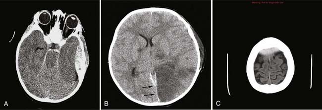
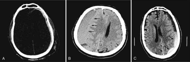
In neurosurgery, CT of the head is used for preoperative and postoperative evaluation of patients for hemorrhage, infarction, hydrocephalus, mass effect, fracture, and postsurgical assessment.8–12 CT is the study of choice to evaluate for acute hemorrhage because it has higher sensitivity and specificity for this indication than MRI does. Intracranial hemorrhage is typically described in terms of its location within the head, such as epidural, subdural, subarachnoid, intraventricular, and parenchymal, with each of these different types of hemorrhages having sufficiently distinct appearances and locations. Epidural hemorrhage has a biconvex contour of its borders (Fig. 17-1A) in relation to the cranial vault and adjacent brain parenchyma and is usually the result of acute trauma associated with an acute fracture across branches of meningeal arteries that hemorrhage into the epidural space. Less commonly, rapid venous hemorrhage into the epidural space may occur and cause an epidural hematoma. The extent of an epidural hematoma is usually limited by periosteal dural insertions at the major sutures. However, an epidural hematoma can extend across the midline in the frontal region anterior to the coronal suture because it is not limited by the dural reflections within the anterior interhemispheric fissure (Fig. 17-1C). A subdural hematoma (SDH) is more common than an epidural hematoma, particularly in older patients, and is generally associated with acute head trauma with or without an associated fracture. Its shape is different from an epidural hematoma because its deeper border against the brain parenchyma is concave and approximates the contour of the adjacent cerebral hemisphere convexity. An acute SDH is typically a result of venous hemorrhage and is not limited by the periosteal dural insertions at the major sutures. However, it is limited by the midline dural reflections within the interhemispheric fissure. The density of the blood in acute, subacute, and chronic SDH changes over time from hyperdense, to isodense, to hypodense (Fig. 17-2). However, a hyperacute SDH or an acute subarachnoid hemorrhage (SAH) in the presence of coagulopathy may sometimes appear isodense or hypodense.
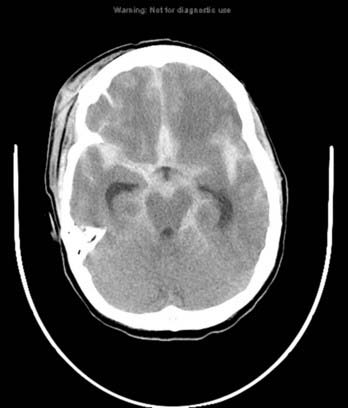
Trauma is the most common cause of SAH, whereas rupture of an intracranial aneurysm is the most common nontraumatic cause of SAH. SAH extends freely within the subarachnoid spaces around the cerebral hemispheres, brainstem, and cerebellum and frequently, by reflux of cerebrospinal fluid (CSF), extends into the intraventricular spaces. It often leads to acute, subacute, or chronic hydrocephalus because the blood products disrupt and obstruct the normal CSF drainage pathways (Fig. 17-3).
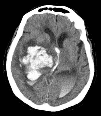
Parenchymal hemorrhages have many causes, including trauma, hypertension, vascular anomalies such as arteriovenous malformation (AVM) or cavernoma, infarction, neoplasm, infection, or vasculitis. They can be small or large and single or multiple, and patient prognosis depends on the cause, number, size, and associated mass effect of the hemorrhage, among other variables (Fig. 17-4).
Computed Tomographic Angiography
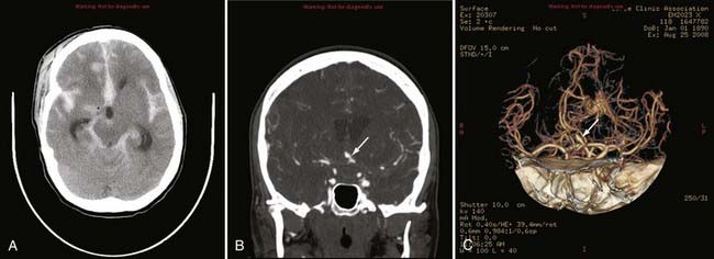
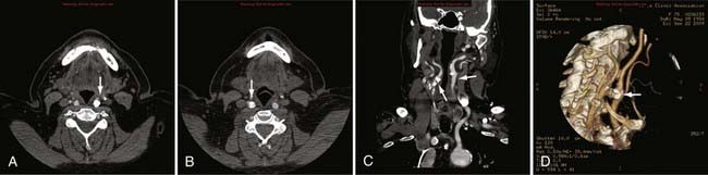
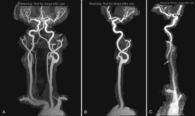
Advances in CT scanner technology have allowed an ever improving capacity for higher resolution images in the submillimeter range with shorter acquisition times. Such technologic improvements have led to imaging techniques such as CTA, which permits relatively noninvasive imaging of the major arteries and veins of the neck and brain after an intravenous injection of iodinated contrast material rather than the traditional catheter-based intra-arterial angiogram technique. This venous injection helps avoid the small risk for complications such as vascular dissection, renal injury, allergic reaction, and iatrogenic embolic strokes associated with traditional catheter angiography. CTA of the neck or brain is performed with a multidetector CT scanner, which allows rapid dynamic imaging of the anatomy of interest after a bolus intravenous injection of iodinated contrast material through a large-bore intravenous catheter (i.e., 18 gauge). Typically, submillimeter axial images are obtained and then reformatted into 2D sagittal and coronal image data sets at 1- to 2-mm intervals. 3D reconstruction images are usually obtained, but interpretation of the study is based primarily on the original axial data set and the 2D sagittal and coronal reformatted images. The diagnostic sensitivity and specificity of CTA approach that of catheter angiography for both the extracranial and intracranial vasculature.13,14 Although CTA cannot entirely replace traditional catheter angiograms, it is a very useful noninvasive screening study for the evaluation, management, and follow-up of patients with definite or possible aneurysms, as well as the evaluation of vasospasm, AVMs, traumatic dissection, stroke, and carotid or vertebral artery atherosclerotic stenosis (Figs. 17-5 and 17-6).15
Perfusion Computed Tomography
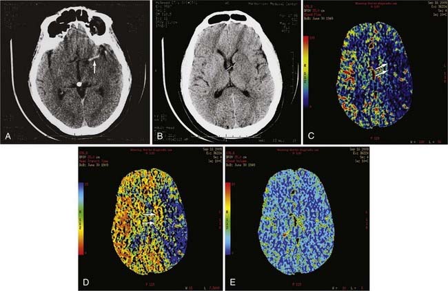
pCT is an example of new advances in imaging that provides physiologic information in addition to anatomic information. pCT is performed with the latest-generation multidetector CT scanners, which allow very rapid CT imaging of a particular anatomy, such as the cerebral hemispheres. During a bolus intravenous injection of iodinated contrast material at a rate of 4 to 5 mL/sec, rapid serial CT images of a chosen volume are obtained in multiple phases over an approximately 1-minute period. At the end of this acquisition, multiphase time-density curves corresponding to each voxel are generated within a 2D image of a multilevel image data set. The data from these images are further postprocessed with a mathematical algorithm that allows displays of the data in color maps representing such physiologic cerebral perfusion parameters as cerebral blood flow (CBF), cerebral blood volume (CBV), and mean transit time (MTT). The CBF, CBV, and MTT maps generated from this CT technique are, in part, quantitative; that is, the numerical values obtained from these images may be expressed in mL/100 g per minute for CBF, mL/100 g for CBV, and seconds for MTT.16 pCT technology has been validated against other proven in vivo techniques such as xenon-enhanced CT and positron emission tomography (PET).17,18
pCT has been used to evaluate acute stroke, central nervous system (CNS) neoplasms, and ischemic sequelae of SAH-related vasospasm. The most common use of the pCT technique is for the evaluation of a patient with an acute stroke. The various color maps of cerebral perfusion help determine the presence of salvageable ischemic penumbra during the first few hours after stroke, which may lead to more aggressive therapy such as an intra-arterial thrombolysis or thrombus extraction to permit rapid recanalization of occluded large intracranial arteries such as the supraclinoid segment of the internal carotid artery (ICA) or M1 segment of the middle cerebral artery (MCA) (Fig. 17-7).
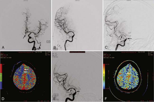
The availability of physiologic data also helps in the diagnosis, management, and treatment of patients with a ruptured aneurysm and subsequent vasospasm, which may contribute to acute or subacute ischemic injury. Evaluation of these patients has typically relied on serial clinical assessment, non–contrast-enhanced head CT, and transcranial Doppler (TCD) ultrasound. There are recognized limitations with this evaluation protocol; in particular, non–contrast-enhanced CT and TCD may not accurately reflect the state of cerebral perfusion at an early enough stage to allow successful intervention for reversal of oligemia and ischemia. Baseline pCT and follow-up pCT can demonstrate the size and extent of brain areas at risk for stroke in patients in a neurological intensive care unit often before symptoms develop and permanent infarction occurs (Fig. 17-8). This early detection of at-risk areas may in some patients permit earlier medical and catheter-based intervention for vasospasm and thus prevent delayed ischemic injury.19–21
Magnetic Resonance Imaging of the Brain
Physics and Techniques of Magnetic Resonance Imaging
History
The interaction of the intrinsic magnetic moment of the nucleus with an externally imposed magnetic field results in the phenomenon known as nuclear magnetic resonance (NMR). Two independent groups, Felix Bloch working with liquid water22 and Edwin Purcell working with solid paraffin,23 detected the hydrogen nucleus resonance in 1946 in bulk matter. Bloch further described the processes and time constants (T1 and T2) by which the resonance would dissipate.24 This set the stage for the eventual development of MRI 30 years later. Between 1946 and 1976, NMR became a useful laboratory tool for probing molecular structure. Laboratory NMR instruments had small spaces for the sample, usually a small test tube. Use of NMR for larger objects, such as humans, required the development of larger magnets with larger sample spaces. The term magnetic resonance imaging is now used rather than NMR to allay patient anxiety about a test that has the word “nuclear” in it.
Basic Physics of Magnetic Resonance Imaging
Creating the Signal
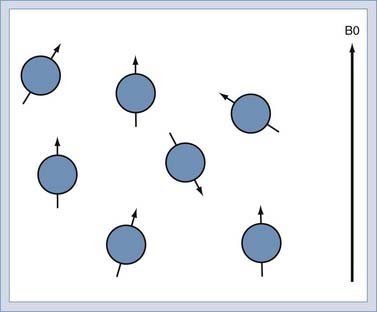
When immersed in the strong, constant magnetic field, the spins in the sample experience a slight polarization. This polarization, known as M0, increases with increasing magnetic field. At 1.5 T, this polarization is very slight, about 1 × 10⁻⁵. This translates to just 10 in 1 million nuclei being polarized.25 The polarization competes with the randomizing effect of the thermal vibration (Fig. 17-9). It is only the polarized nuclei that contribute to the MR signal; hence, MRI systems with higher field strength produce better images.
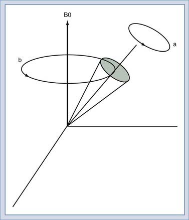
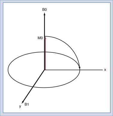
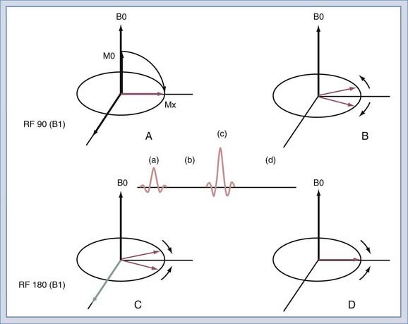
We will use the classic model created by Bloch to describe the motion of the spins. Spins that align with the main field precess around the direction of the main field in a manner similar to the spinning of a toy top (Fig. 17-10). The rate of this precession is a product of the intrinsic magnetic moment (the gyromagnetic ratio) of the spin and the strength of the main magnetic field. The rate of precession is known as the Larmor or resonant frequency.26 The spins aligned along B0 are rotated into a plane transverse to the direction of the main magnetic field by the action of a time-varying magnetic field called B1 (Fig. 17-11). The B1 field is created by the radiofrequency (RF) transmitter and the antenna, known as the RF coil. The frequency of the B1 field matches the Larmor frequency of the spins. The B1 field is of brief duration, typically 1 to 10 msec, and is thus referred to as an RF pulse. The angle through which the spin is rotated is called the flip angle. The flip angle depends on the duration and amplitude of the RF pulse.
Detecting the Signal
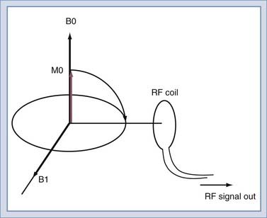
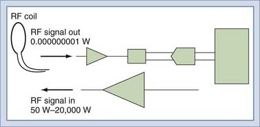
To detect the MR signal, an RF coil is placed as shown in Figure 17-12. This may be the same coil used to transmit the B1 pulse. A time-varying magnetic field will be created at the coil by the magnetic field of the precessing spins (rotated in the transverse plane) as they pass by the RF coil. Magnetic induction (Faraday’s law) causes the RF coil to produce an electric current, which can then be amplified and detected (Fig. 17-13). An interesting and important disparity should be noted. The amount of power used to produce the RF pulse is in the range of 100 to 20,000 W. The signal that is received from the object is on the order of 10−12 W. This received signal is no greater than the signals from radio or television stations, among other sources. To prevent interference from these external sources, MRI systems are enclosed in electrically shielded rooms, which are six-sided copper boxes.
Physics: Localizing the Signal
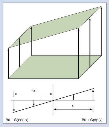
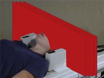
To this point, the sample has been polarized and excited and a signal detected, but the location of the spins that created the signal remains unknown. Suppose that two objects are in the magnetic field, both of which create a signal. To force each object to give off a unique signal, the magnetic field can be modified to vary as a function of position along the x-axis (Fig. 17-14). The resonant frequency of the spins is a function only of the magnetic field at that point in space. Thus, the spatial origin of the signal can be determined by the frequency of the received signal. In practice, this is done by creating a linear gradient that adds or subtracts to the main field as a linear function of offset from the origin. An MRI system has three gradients: x, y, and z. The gradient system serves two purposes in the MRI system. The first is to limit the excitation to a plane or slab (Fig. 17-15). If an RF pulse is transmitted during the time that a gradient is applied, only a slice or slab will be excited, the thickness of which depends on the amplitude of the gradient and the bandwidth of the RF pulse. The second purpose is to encode the spatial location of spins to form the MR image. In a slice, the two directions of encoding required are frequency and phase. Location along the frequency-encoding axis is accomplished by applying a gradient during the signal readout time. The orthogonal axis is encoded by applying a gradient somewhere between the time of excitation and reception and is called phase encoding. One unique value of phase encoding is applied every time that the readout gradient is applied. Thus, the excitation and readout must be repeated to make an image. The rate at which the excitation is repeated is the TR time.
The Origin of Image Contrast
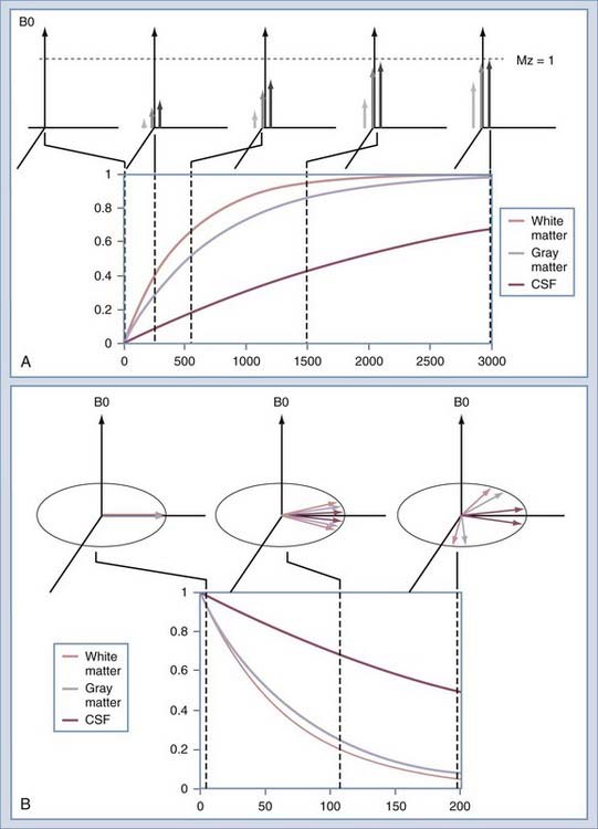
The intensity of a voxel in an image arises from the three principal factors. The first is the number of protons in the voxel, known as proton density. If this were the only image mechanism, MRI would be little more than a CT scanner. However, intensity in the voxel also depends on the relaxation rates of the spins. The first is T1, or the longitudinal relaxation rate (Fig. 17-16A). After excitation, the magnetization in the slice returns along the axis of the main magnetic field by interaction with other nonmoving hydrogen spins, typically those attached to large molecules. The magnetization returns along B0 as an exponential function of the ratio of T1 and the rate at which the excitation is repeated, or TR. The second relaxation rate is T2 (Fig. 17-16B). This rate describes the rates at which spins that have been excited into the transverse plane lose coherence. Each spin precesses at a rate that is determined by the magnetic field at the location of that spin. Macroscopic and microscopic field gradients, created by differences in the magnetic susceptibility of tissue, cause some of the excited spins to precess faster and some slower. Eventually, the spins are spread out uniformly, which produces no signal in the RF coil used to detect the spins.
Spin Echo
After the spins have been rotated into the transverse plane by the initial 90-degree RF pulse (Fig. 17-17A), they begin to lose coherence because of the effects of local inhomogeneities (contributed by changes in tissue), inhomogeneities secondary to imperfections in the B0 field, and diffusion of water molecules (Fig. 17-17B). If a second RF pulse is transmitted at twice the amplitude of the first pulse, the relative direction of the spins can be reversed (Fig. 17-17C). Then, at the echo time, the spins will have nearly regained coherence (Fig. 17-17D). The effects of magnetic field inhomogeneities are thus cancelled out. One loss, that caused by diffusion, cannot be reversed but is usually negligible in routine imaging. The resulting coherence produces the spin echo as described by Erwin Hahn in 1950.27 If the 180-degree pulse is not used, the signal decreases with increasing echo time as T2*. With the 180-degree pulse included, the decrease is T2, with T2 always being greater than T2*.
The spin echo sequence is the mainstay of routine clinical imaging. By adjusting TE and TR times, proton density–, T1-, or T2-weighted images can be selected (Table 17-1).
| SHORT TE | LONG TE | |
|---|---|---|
| Short TR | T1 weighted | Mixed contrast—do not use |
| Long TR | Proton density weighted | T2 weighted |
TE, echo time; TR, repetition time.
Gadolinium Contrast
Exogenous contrast enhancement is now a routine part of MRI. The most widely used is a gadolinium chelate. The gadolinium atom is strongly paramagnetic and acts to shorten the T1 relaxation time of nearby water protons in blood.28 The agent does not pass the blood-brain barrier and thus becomes a marker for abruptions in the blood-brain barrier caused by neoplasm, infection, trauma, and infarction. The T1-shortening effect is also used for rapid MRA, which is performed by using a fast scanning protocol after the bolus injection of a contrast agent. In the brain, bolus injection of gadolinium with repeated echo planar imaging (EPI) has been used to image perfusion29 and the blood volume of tumors.30
Fast Spin Echo
Fast spin echo (FSE) sequences decrease scan time by increasing the efficiency of data collection.31 The increased efficiency can be used to either decrease scan time or increase the signal-to-noise ratio of the resulting images. Improved scan efficiency has resulted in the frequent application of FSE sequences in radiology, particularly in imaging of the CNS.
To understand this improved efficiency, it is necessary to understand how the data are collected. In a conventional spin echo sequence (Fig. 17-18A), a single line of k-space samples (called a view) is collected. For images that are not fractional excitation, the number of views is equal to the matrix size in the phase that encodes image direction. The next view is collected at TR time later, when the sequence is repeated. The entire k-space matrix must be collected before the images can be reconstructed. The TR time is set in accordance with the desired contrast (Table 17-1). The FSE sequence collects multiple views in each TR time (Fig. 17-18B). The number of views collected per TR time is known as the echo train length (ETL). An FSE sequence with an ETL of 4 has a total scan time a fourth that of a conventional spin echo sequence with equivalent TR. The ETL can be equal to the number of views in the sequence. This allows the entire image to be collected in a single TR time.
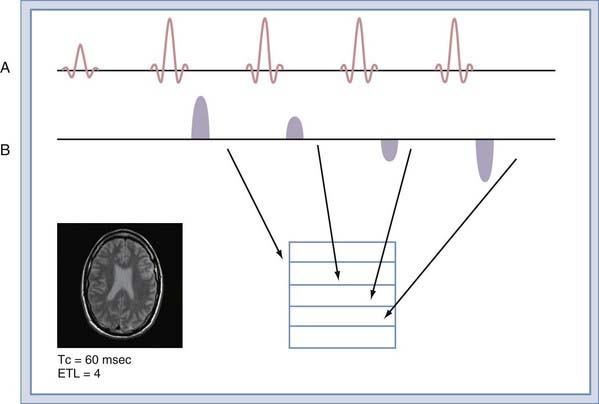
The improved efficiency of FSE sequences comes at the expense of image contrast purity because each view is collected at a different echo time (Fig. 17-18B). The effect is to create image blurring that worsens with increasing ETL or decreasing tissue T2. The relatively long T2 times of tissues in the neuraxis allow ETL values of 16 to be used routinely. To image uncooperative patients, single-shot FSE sequences can be used, but with some increase in image blurring.
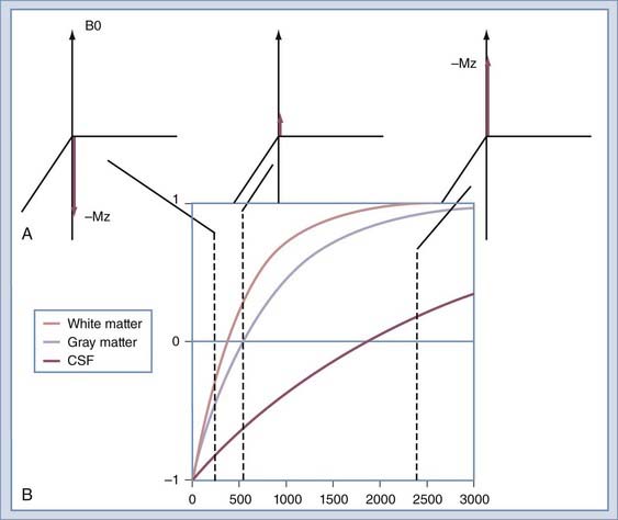
Inversion Recovery
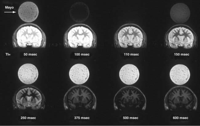
Image contrast can be further manipulated by transmitting a 180-degree RF pulse before the pulse sequence. The effect of using this pulse is to rotate the spins from their orientation along +z to −z (Fig. 17-19A). The longitudinal magnetization (Mz) signal regrows from −z to +z at a rate determined by the T1 of the spins. The regrowth is plotted in Figure 17-19B for several tissues. If the 90-degree RF pulse is transmitted at the time at which Mz is 0, the tissue will produce no signal. Inversion recovery can be used to increase contrast between structures, such as gray and white matter, or to null signals that arise from protons of a known T1. A coronal image of a volunteer imaged at multiple T1 times is shown in Figure 17-20. The round object above the volunteer’s head is a jar of mayonnaise. Fluid-attenuated inversion recovery (FLAIR) imaging32 uses this method to null CSF while preserving signal from edematous tissue. The inversion pulse may be applied to a spin echo or gradient echo sequence.
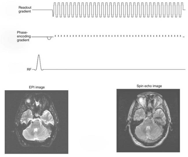
Echo Planar Imaging
The readout gradient used to form the echo in a gradient echo sequence can be repeated to collect additional k-space views in a manner similar to FSE.33 Between repetitions of the readout gradient, a small phase-encoding gradient is applied that allows a different view to be collected during the subsequent readout gradient (Fig. 17-21). Only a single excitation is used to collect all the views in k-space. The entire image can be collected in approximately 40 msec. Applications that are highly sensitive to even minor patient motions use this sequence. Like FSE, EPI suffers from blurring caused by acquiring views at different echo times, but without rephasing of the RF 180-degree pulses. This effect limits the resolution obtainable. Although an FSE image may use a matrix of 256 × 256, EPI is limited to 128 × 128 or more typically 64 × 64 over the same field of view. Despite these limitations, EPI is essential for diffusion, perfusion, and functional MRI (fMRI).
Diffusion-Weighted Imaging
Diffusion of water in the brain depends on the integrity of the cellular membrane and the osmotic balance of the neurons and astrocytes.34 In ischemic processes, the diffusion of water first decreases because of cellular swelling and thus decreases the extracellular space. During recovery and into the chronic stage, the loss of cell wall integrity causes the diffusion to increase.
Perfusion-Weighted Imaging
Two main approaches are taken to measure tissue perfusion. Both methods use EPI sequences because like diffusion, the effect can be easily degraded by minor patient motion. The first method for imaging tissue perfusion is to create an endogenous contrast. This is done by presaturating the blood flowing into the organ with an RF pulse. EPI of the organ is performed with the presaturation on and off. By subtracting the two images, a tissue perfusion image is created.35 The second method is by bolus injection of contrast material while repeatedly performing EPI. Time course images from EPI are then fitted to a model of the response of the tissue to the presence of the contrast agent, and an image of perfusion is made. This method is also known as a dynamic susceptibility contrast technique and requires a rapid intravenous bolus injection of gadolinium contrast material at a rate of 4 to 5 mL/sec, usually through an 18-gauge intravenous catheter, followed by normal saline injection. Manual or automatic postprocessing is required to generate color maps of various parameters of cerebral perfusion, such as CBV, CBF, mean time to enhance, and MTT.
Spectroscopy
The resonant frequency of a spin is determined not only by the B0 magnetic field and its associated imperfections but also by the molecule of which the nucleus is a part. The effect is slight, but not negligible. This phenomenon is known as chemical shift; that is, the chemical microenvironment of a given nucleus results in a slight change in the resonance frequency of the nucleus from that expected in its pure state. The difference between the resonant frequencies of the protons in water and the hydrogen atoms in the methylene groups in lipid are about 3.5 ppm. This translates to a difference of about 220 Hz for operation at 1.5 T. Between the water proton and fat proton resonances lie resonances of other moieties of interest in the brain. These include myoinositol, a sugar phosphate; choline, a key indicator of membrane turnover; creatine and phosphocreatine, part of the energy pool; glutamate and glutamine, the primary excitatory neurotransmitter and its astrocyte-recycled counterpart; N-acetyl aspartate (NAA), a key indicator of neuronal health; and lactate, an indicator of a shift to anaerobic metabolism. A spectrum of the resonances of the protons in these compounds is shown in Figure 17-22A. These resonances are included in every MR image of the brain. However, the concentration of each is lower than that of water by a factor of 5000 to 10000. To detect the resonances of the metabolites thus requires much larger voxels than imaging does: 2 cm3 versus 1 mm3 in imaging.
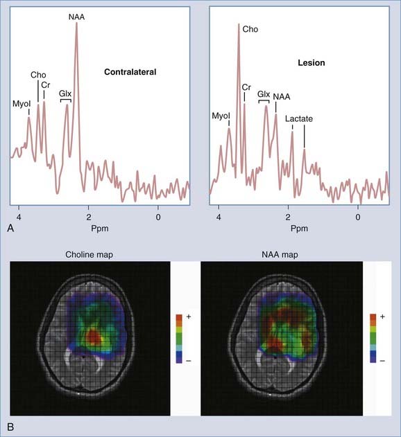
Two principal methods are used to collect spectroscopic data. The first, single-voxel spectroscopy, selects a voxel by using three successive RF pulses and then reads out the signal from the entire voxel. The second, chemical shift imaging, selects a larger volume or slice with one or more RF pulses. Phase-encoding gradients are then applied in one to three directions to yield 2D or 3D spectroscopy data sets. Reconstruction allows the selected region to be subdivided into separate voxels. An individual spectrum can then be extracted from a voxel, or a resonance may be selected and an image made of that resonance. Such 2D and 3D data sets can be postprocessed to generate color maps of metabolite distributions within the volume of brain evaluated with spectroscopy (Fig. 17-22B).
Clinical proton MR spectroscopy (MRS) has been commercially available for more than a decade. Nevertheless, MRS remains somewhat limited in use and is found in select academic medical centers and some large community hospitals because of the level of complexity in acquisition and postprocessing of data. However, in centers with active spectroscopy programs, clinical MRS can add value in the diagnosis, follow-up, and thus management of patients with various neurological diseases, including epilepsy, neoplasms, demyelinating disorders, metabolic diseases, and ischemic diseases.36,37 The clinical applications of proton spectroscopy to neoplasms, stroke, and epilepsy are discussed later in this chapter.
Functional Magnetic Resonance Imaging
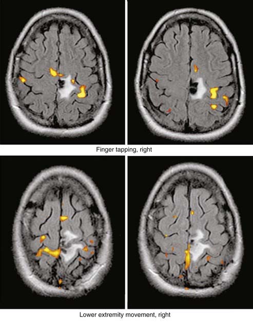
fMRI is used to image the change in the ratio of oxyhemoglobin to deoxyhemoglobin in cerebral blood in response to a stimulus.38 Changes in the ratio within activated cortical structures are taken to be indicative of changes in the oxygen extraction fraction.39 These changes are thought to occur in response to cortical function and the resulting upregulation of local metabolism. The change in the oxyhemoglobin-to-deoxyhemoglobin ratio alters the magnetic susceptibility of the blood because deoxyhemoglobin is less paramagnetic than oxyhemoglobin. This difference is manifested as a change in T2* in activated tissue.
The effect is slight; at 1.5 T the change in image intensity is less than 6%. To preclude interference from patient motion, the data are collected with EPI techniques. Images are repeatedly acquired at the same location over the course of the application of a stimulus pattern. By using the a priori knowledge of the stimulus pattern and cross-correlating it with the time course intensity data, a functional image may be made (Fig. 17-23).
Clinical Magnetic Resonance Imaging
Neoplasms
Gliomas
Gliomas are the most common primary brain neoplasms in both adults and children and represent approximately half to two thirds of all brain tumors, respectively, encountered in these populations. Gliomas are usually categorized into four distinct histologic subgroups—astrocytomas, oligodendrogliomas, ependymomas, and choroid plexus tumors, which include the more common papillomas and rare carcinomas and xanthogranulomas.40,41
The MRI appearances of gliomas are quite varied, but in some cases these neoplasms can have a set of very distinct appearances and location that permit a correct preoperative radiologic diagnosis. In other cases, the MRI appearance is not specific and several differential diagnoses have to be entertained preoperatively. MRI appearances can also vary according to the neoplasm’s histologic grade: lower grade tumors usually exhibit little or no peritumoral vasogenic edema, whereas higher grade tumors demonstrate prominent vasogenic edema associated with a local/regional mass effect or herniation, or both.42,43 However, the sensitivity and specificity of MRI in assessing the degree of histologic anaplasia of a given neoplasm are limited.
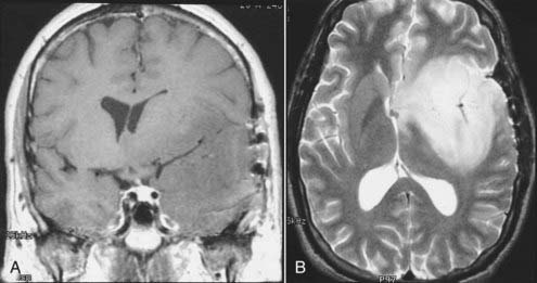
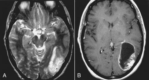
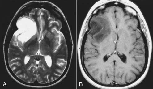
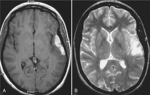
Astrocytomas represent the largest subgroup of gliomas (about 20% to 30% of all gliomas). The histologic subtypes of astrocytomas (e.g., fibrillary, protoplasmic, or gemistocytic) cannot be distinguished by MRI. However, certain subtypes, such as the cystic pilocytic astrocytomas typically found in the cerebellum in children and subependymal giant cell astrocytomas in patients with tuberous sclerosis, may be diagnosed preoperatively by MRI because of their typical appearance, location, and clinical features. Astrocytomas are usually hypointense to normal brain tissue (cortex and white matter) on T1-weighted images and mildly to significantly hyperintense to normal brain on T2-weighted and FLAIR images. Although not completely reliable, in general, low-grade astrocytomas are usually well circumscribed and exhibit no or minimal peritumoral edema, whereas the higher grade anaplastic or glioblastoma multiforme varieties are usually more infiltrative in appearance with less well defined borders and are associated with significant surrounding edema. Low-grade tumors are generally homogeneous in signal characteristics on both T1- and T2-weighted images, whereas higher grade tumors are more likely to be heterogeneous; this reflects the heterogeneity observed by histology associated with the cystic and necrotic changes typically found in these tumors (Figs. 17-24 and 17-25). Rarely, certain astrocytomas demonstrate signal intensity characteristics that are similar or identical to those of CSF on T1- and T2-weighted images.42,43 Some of these tumors are in fact predominantly cystic in composition, which explains their signal characteristics, but some are solid neoplasms whose parenchymal composition and organization (e.g., microcysts) mimic CSF signals on MRI. Therefore, with MRI, unlike CT, lesions that appear to have the same signal as that of CSF may not be cystic.
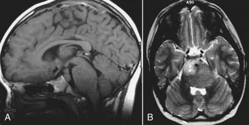
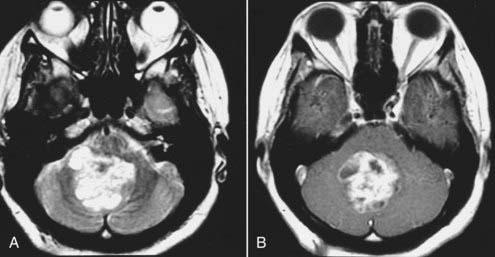
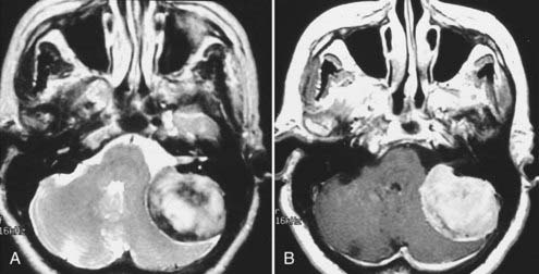
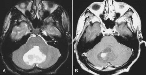
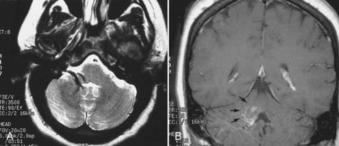
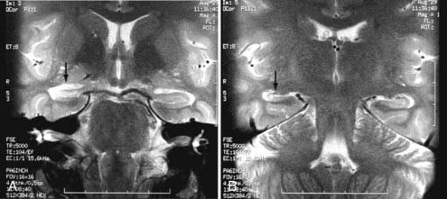
Brainstem gliomas, which are usually of a fibrillary histologic type and more common in children, appear as a poorly defined mass within the brainstem with diffuse enlargement. They frequently demonstrate exophytic growth with partial or complete circumferential encasement of the basilar artery (Fig. 17-26).44,45 Gliomatosis cerebri, in which the neoplasm is diffusely infiltrating without a discrete mass, is another astrocytoma subtype. The patient may often have nonfocal neurological findings such as headache, decline in mental status, or changes in personality; on MRI, extensive involvement of one or both cerebral hemispheres is observed, with diffusely abnormal T2 hyperintensity involving the subcortical and deep white matter.
Enhancement of astrocytomas on gadolinium-enhanced T1-weighted images can be quite variable. In general, higher grade tumors demonstrate more prominent enhancement than do lower grade tumors; however, exceptions do occur.46 Therefore, the presence or absence of significant enhancement in a neoplasm, by itself, should not be used to suggest the degree of anaplasia. Interlobar, interhemispheric, or transtentorial macroscopic extension of astrocytomas (or any combination of such extension) and associated vasogenic edema can readily be seen on MRI, especially on T2-weighted and FLAIR images. However, MRI is more limited in the assessment of microscopic tumor infiltration at the tumor margins and in defining the border between the neoplasm and its non-neoplastic vasogenic edema. Contrast-enhanced T1-weighted images can improve the sensitivity of MRI both preoperatively and postoperatively when looking for recurrence. This might be further improved by MRS either in single-voxel or in 2D multivoxel (chemical shift imaging) forms. On MRS, a significantly elevated amplitude of the choline peak relative to that of creatine or NAA suggests a recurrent neoplasm, whereas absence of elevated choline on the background of mobile lipids and lactate would favor radiation necrosis or postsurgical changes, or both (Fig. 17-27).47–49 Additional new MRI techniques such as perfusion MRI and activation fMRI are now being used for preoperative evaluation of tumor and for surgical planning (Fig. 17-28).50–53
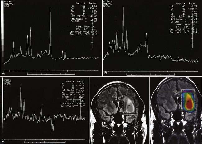
FIGURE 17-27 A, Single-voxel magnetic resonance (MR) spectra (TR = 2000 msec, TE = 35 msec) from an experimental phantom showing the expected normal appearance of proton (1H) MR spectroscopy, except for the double lactate peaks. The dominant peak is for N-acetyl aspartate (NAA). Peaks for creatine, choline, and myoinositol are also seen. Refer to the labeled normal spectra from the contralateral hemisphere in Figure 18-22A. B, Abnormal single-voxel MR spectra (TR = 2000 msec, TE = 35 msec) from a patient with a frontal lobe mass showing reduced NAA amplitude and an increased amplitude of choline, consistent with a neoplasm. C, Single-voxel MR spectra (TR = 2000 msec, TE = 135 msec) from a different patient with a neoplasm showing a similar abnormal pattern and double lactate peaks, indicative of the presence of anaerobic metabolism and production of lactate by the neoplasm. D, Color metabolite map for choline from multivoxel MR spectroscopy (TR = 2000 msec, TE = 144 msec) in a patient with a progressive high-grade astrocytoma demonstrating an abnormally increased concentration of choline (displayed in red) in the left inferior frontal lobe.
Oligodendrogliomas, which arise from oligodendrocytes, are tumors of adults and have a peak incidence in the fourth to sixth decades. When made up predominantly or purely of oligodendrocytes, they behave in a benign manner. However, when the tumors are of mixed cell origin and contain both astrocytic and oligodendrocytic components, the astrocytic component often degenerates into a more anaplastic astrocytoma at recurrence. This occurs in about half of oligodendrogliomas. Calcifications are common in oligodendrogliomas, and histologically about 70% contain calcification.40 On CT, about 30% to 40% of these tumors contain visible calcification. On MRI, calcifications are usually hypointense on T1- and T2-weighted images, but microcalcifications can demonstrate hyperintensity on T1-weighted images (Fig. 17-29). However, oligodendrogliomas, mixed oligoastrocytomas, and astrocytomas cannot be reliably differentiated by their MRI appearances.54
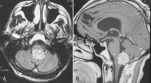
Ependymomas have protean MRI appearances with variable signal intensities on T1- and T2-weighted images, consistent with the variable cellularity and histologic composition found in these tumors. They are typically hypointense on T1- and hyperintense on T2-weighted images, but calcification or cystic or hemorrhagic components will often result in a variable heterogeneous MR signal and enhancement (Fig. 17-30).55 Ependymomas can be found both in a supratentorial location typically within the lateral ventricles and in an infratentorial location within the fourth ventricle. They can demonstrate intraventricular or predominantly extraventricular appearances. A subtype called a subependymoma is typically manifested as a periventricular parenchymal mass.
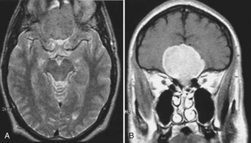
Choroid plexus papillomas and carcinomas can develop within the ventricular system. In children, they typically occur in the atrium of the lateral ventricles, whereas in adults, they are more common within the fourth ventricle. They are generally T1 hypointense and T2 isointense to hyperintense with prominent enhancement (Fig. 17-31). Papillomas are well circumscribed and lobulated in contour, which corresponds to the classic “cauliflower”-like appearance in gross pathology.56 Choroid plexus papillomas are frequently associated with communicating hydrocephalus. There is debate about the etiology of the hydrocephalus in these patients, but it probably represents some combination of overproduction of CSF by the tumor and obstruction to normal CSF absorption by arachnoid granulations as a result of cellular debris shred from the papilloma.
Meningiomas
Meningiomas are the second most common primary brain neoplasm. They occur at any age and in either sex but are usually found in middle-aged to older women. Meningiomas arise from arachnoid cap cells and are commonly found over the parasagittal cerebral convexity, sphenoid wing, parasellar region, tuberculum sella, olfactory groove, and cerebellopontine angle region. On MRI, meningiomas are usually isointense to gray matter on both T1- and T2-weighted images and can therefore be overlooked on a screening MRI study obtained without contrast enhancement.57 Certain histologic subtypes such as syncytial and angioblastic meningiomas demonstrate hyperintensity on T2-weighted images.58 When gadolinium contrast is administered, meningiomas are remarkably easy to detect because they exhibit reliably prominent and generally homogeneous enhancement (Fig. 17-32).59 They are often associated with an enhanced thickened dura along the lateral margins of the tumor that is known as a “dural tail.”60 In some cases these dural tails represent the margins of tumor extension, whereas in most cases they represent reactive dural enhancement without tumor infiltration.61 A dural tail is not unique to meningiomas and can be observed in other neoplastic and non-neoplastic processes, including exophytic gliomas, dural metastases, lymphoma, and granulomatous infections. Meningiomas sometimes have areas of necrosis, macroscopic calcification, hemorrhage, or cystic changes. Such findings lead to some heterogeneity of signal and enhancement (Fig. 17-33). Most meningiomas have relatively small amounts of vasogenic edema and are frequently found with no significant edema despite their large size. In some cases, however, they are associated with a large amount of vasogenic edema that resembles the edema observed with high-grade gliomas.58
Pituitary Adenomas
T1 weighting with gadolinium enhancement is the most important imaging sequence for evaluating pituitary adenomas. The images should include thin (2 to 3 mm) coronal images through the sella turcica with a small field of view. In microadenomas, dynamic imaging of the gland should be done with a series of thin three to four coronal images rapidly obtained over a period of 2 to 3 minutes during bolus intravenous injection of gadolinium.62 This technique is used to identify a relatively slowly enhancing microadenoma within a rapidly and homogeneously enhancing normal pituitary parenchyma. This pattern of enhancement results in the microadenoma being delineated from normal parenchyma as a hypoenhancing/hypointense lesion on contrast-enhanced T1-weighted images. Other imaging findings associated with a microadenoma include deviation of the infundibulum away from the side of the gland containing the adenoma, asymmetric convexity of the superior border of the gland, or abnormal contour of the sella turcica floor.63
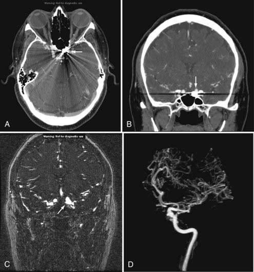
Additional imaging sequences, including T1-weighted sagittal images with contrast enhancement and T2-weighted coronal images, are valuable to define tumor extension and associated parenchymal changes, if present, of macroadenomas. 3D time-of-flight (TOF) MRA of the cavernous sinus and the circle of Willis can also better define the relationship between the macroadenoma and the ICAs and the M1 and A1 segments of the middle and anterior cerebral arteries, respectively (Fig. 17-34).
Metastatic Neoplasms
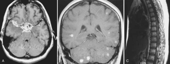
MRI with gadolinium enhancement is the most sensitive imaging technique for evaluating CNS metastasis. MRI is superior to CT in tissue contrast, ease of multiplanar evaluation, and absence of artifacts, especially in the posterior fossa.64 Neoplasms that metastasize to the brain have a wide variety of MRI appearances that depend on their cells of origin, cellular density, and associated pigments (e.g., melanin or hemorrhage). Metastatic lesions are typically localized at the gray-white matter junction in the cerebral hemispheres and are more frequent in the distribution of the anterior than the posterior circulation; this probably reflects differences in blood flow (Fig. 17-35). Typically, the parenchymal lesions are isointense to hypointense on T1-weighted images and isointense to hyperintense on T2-weighted images, with prominent surrounding vasogenic edema relative to lesion size.65 These lesions enhance moderately to prominently and are usually multiple. Some metastatic lesions, such as those from thyroid carcinoma, renal cell carcinoma, choriocarcinoma, and melanoma, are often hemorrhagic and demonstrate T1 and T2 signal changes corresponding to subacute and chronic blood breakdown products. Metastases from adenocarcinomas from lung, breast, or colon cancer are occasionally associated with neoplastic cysts (Fig. 17-36). In meningeal carcinomatosis, the metastases involve the meninges and appear as a diffusely thickened enhancement of the pia or pachymeninges (Fig. 17-37) or as multiple, dural-based nodular-enhancing lesions.66
Schwannomas
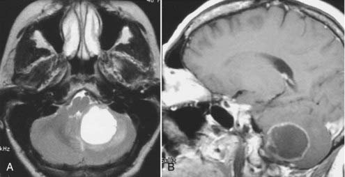
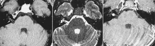
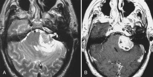
Intracranial schwannomas arise from the Schwann cells that envelop the cranial nerves as they exit the intracranial compartment through various canals and foramina. They are more often found within the posterior fossa. The most common intracranial schwannomas arise from the vestibular divisions of the eighth cranial nerve. They are typically located within the internal auditory canal (IAC) with extension through the porus acusticus into the cerebellopontine angle.67 Depending on the size of the neoplasm, a variable degree of brainstem distortion or compression is observed together with minimal, if any, intra-axial brain edema. Tumor growth may cause bone erosion and widen the IAC and the porus acusticus. Vestibular schwannomas are usually isointense to hypointense to brain tissue on T1-weighted images and hyperintense to brain on T2-weighted images with prominent enhancement after intravenous gadolinium injection. When they are small (e.g., intracanalicular tumor), vestibular schwannomas typically enhance homogeneously (Fig. 17-38). However, with an increase in tumor size, cystic and necrotic foci can develop, which then contribute to more heterogeneous MRI signal characteristics and enhancement patterns (Fig. 17-39).
Vestibular schwannomas are the most common mass lesions in the cerebellopontine angle and represent about 75% of all masses in this location. The next most common mass in the cerebellopontine angle is a meningioma. Meningiomas tend to exhibit more intermediate T2 signal characteristics than do vestibular schwannomas and infrequently extend into the porus acusticus. Although the epicenter of a vestibular schwannoma is at the porus acusticus, a meningioma in this location is located eccentric to the porus acousticus.68
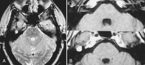
Other intracranial schwannomas include those from the trigeminal (cranial nerve V), facial (VII), glossopharyngeal (IX), vagus (X), spinal accessory (XI), and hypoglossal (XII) nerves. Of these, trigeminal nerve schwannomas are the most common. Facial nerve schwannomas often appear as a lytic, enhancing mass in the petrous temporal bone in the region of the geniculate ganglion (Fig. 17-40).69 The origin of a schwannoma that arises from cranial nerve IX, X, XI, or XII in the caudal aspect of the posterior fossa is difficult to ascertain on preoperative MRI and may be obvious only at the time of surgery.
Primitive Neuroectodermal Tumors
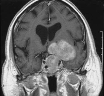
Primitive neuroectodermal tumors (PNETs) were first defined to describe large, solid hemispheric neoplasms made up of undifferentiated cells, often found in infants and young children, that could not be designated, because of their locations, as a retinoblastoma, medulloblastoma, pineoblastoma, or ependymoblastoma. However, most pathologists are of the opinion that these various neoplasms are similar in their histopathology. Therefore, the designation PNET is used to describe all these undifferentiated, primitive neoplasms found in children and young adults.40 In the posterior fossa, PNETs arise from the germinal matrices surrounding the fourth ventricle in children and along the anterolateral cerebellar hemisphere in young adults. They can also occur in the supratentorial compartment as intraventricular or intra-axial masses. PNETs are made up of small round cells and are hypercellular with a high nuclear-to-cytoplasm ratio. These characteristics contribute to their MRI signal characteristics, which are slightly hypointense to isointense to brain tissue on T1- and isointense on T2-weighted images. They demonstrate moderate to prominent enhancement on contrast-enhanced T1-weighted images. PNETs are typically homogeneous solid masses but can have cystic or necrotic components that result in more heterogeneous signal and enhancement characteristics (Fig. 17-41).70
Infections
MRI evaluation for meningitis is limited by its marginal sensitivity. With the advent of the FLAIR pulse sequence and especially with gadolinium-enhanced FLAIR studies, increased sensitivity for meningeal diseases is reported, but further large-scale prospective studies are required. A normal brain MRI study does not exclude meningitis. Therefore, the diagnosis of meningitis should still be made by chemical and bacteriologic examination of CSF. However, in a patient with high suspicion or a proven meningeal infection, MRI is valuable and can help ascertain the degree of involvement and the presence of any parenchymal involvement (i.e., encephalitis, infarction, or abscess formation). MRI also can help monitor a patient’s response to therapy if an objective parameter, in addition to the clinical findings, is required.71
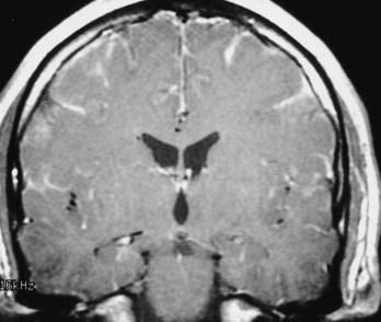
Viral meningitis, when visible on MRI, is typically manifested as diffuse meningeal enhancement on gadolinium-enhanced T1-weighted images (Fig. 17-42). When encephalitis is present (e.g., herpes encephalitis), the involved parenchyma reflects the presence of cytotoxic and vasogenic edema with hypointense T1 and hyperintense T2 signal characteristics involving both gray and white matter (Fig. 17-43). Effacement of local cortical sulci, hemorrhage, and prominent leptomeningeal enhancement may also be present.72
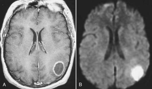
Bacterial meningitis is often associated with prominent diffuse meningeal enhancement. It is typically hematogenous, but it also results from direct extension of infections in the adjacent paranasal sinuses or mastoid air cells. Complications of bacterial meningitis include subdural empyema, infarction, and parenchymal abscess. An abscess is seen on T1-weighted images as a mass with a central nonenhancing or slightly enhancing T1 hypointense cavity with an enhancing wall of variable and irregular thickness that is surrounded by T1 hypointense and T2 hyperintense edema. The central cavity is typically hyperintense on T2-weighted images, but it can be isointense or hypointense, depending on its contents.73 However, these MRI appearances are similar to those observed with a necrotic neoplasm. MRI findings can be crucial in distinguishing an abscess from a necrotic neoplasm when other clinical or laboratory data are lacking. The enhancing wall of an abscess cavity is typically thinner along its medial/deeper aspect and thicker along its lateral/superficial aspect. The extent of associated edema may be smaller with an abscess, whereas a necrotic brain neoplasm such as glioblastoma multiforme usually has a large area of surrounding vasogenic edema.74 Newer MRI techniques such as MRS and diffusion-weighted imaging (DWI) can help differentiate abscesses from necrotic neoplasm. In MRS, spectroscopic evaluation of an abscess reveals several amino acid signatures and abundant lactate and mobile lipids. These, however, are also observed in necrotic neoplasms. On DWI, an abscess cavity typically has a restricted diffusion pattern with a low apparent diffusion coefficient (ADC) and hyperintense signal on diffusion-weighted images (Fig. 17-44).75,76 By contrast, a cystic/necrotic neoplasm has a relatively increased ADC with hypointense signal on diffusion-weighted images.
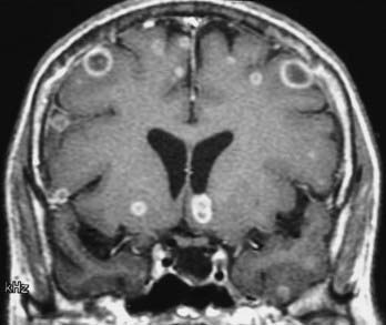
MRI can be used to image other infections such as tuberculosis, fungal infections, and cysticercosis. Tubercular meningitis usually involves the basal meninges and typically extends into the Virchow-Robin perivascular spaces of the basal ganglia, which may cause lacunar infarctions (Fig. 17-45).77–79 Fungal infections involve the brain by direct extension from contiguous structures such as the paranasal sinuses, orbits, and mastoid or by a hematogenous route. These infections are usually found in diabetic patients or immunocompromised individuals. Meningitis and encephalitis with parenchymal abscesses are possible. In Aspergillus infection, the fungus has a propensity for vascular invasion, which results in hemorrhagic transformation of encephalitic foci.80,81 Cysticercosis is an infection that results from infestation with a pork tapeworm. When these parasites die within the brain, parenchymal reaction to the dying parasites contributes to the edema, enhancement, and calcification seen on imaging. Cysticercosis appears as small, parenchymal lesions with punctate calcifications, intraventricular masses, or multiple lobulated T1 hypointense masses that expand the subarachnoid spaces (racemose form) (Fig. 17-46).82,83
Stroke and Vascular Diseases
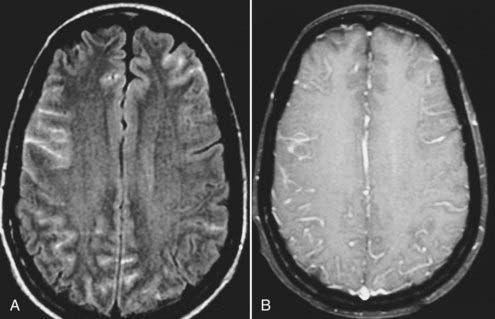
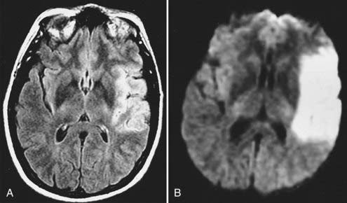
Echo planar DWI has even further decreased the time required for MRI visualization of an acute stroke.84 In animal models, DWI can demonstrate large vascular territory infarctions (e.g., ICA or MCA) within minutes after vessel occlusion.85 In humans, acute infarctions can be demonstrated on DWI within 30 minutes to 1 hour. This implies that most acute infarctions should be visible on DWI by the time that a patient arrives at the hospital after the onset of stroke (Fig. 17-47).86 Once present on MRI, the hyperintense infarction on DWI persists for approximately 2 weeks, depending on size and location and the diffusion sensitivity factor (i.e., b value) that is used to obtain the diffusion-weighted images. After this period, subtle hyperintensity may remain and corresponds to the areas of abnormal hyperintensity on T2-weighted and FLAIR images. The degree of such hyperintensity on DWI is much less than that observed with an acute infarction. This phenomenon is known as the “T2 shine-through” effect and should not be confused with an acute infarction.87
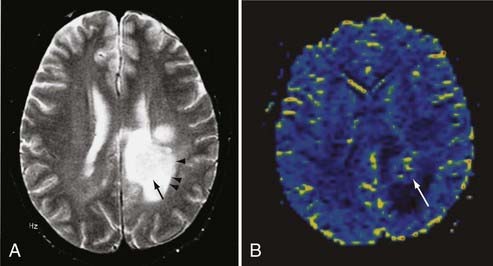
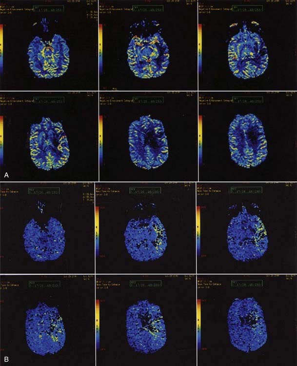
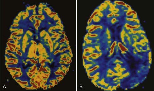
Perfusion MRI, in the form of dynamic susceptibility imaging, shows promise in evaluation of cerebral perfusion, expressed as relative CBV or MTT. Again, using an echo planar technique, several hundred images of the brain can be obtained in less than 2 minutes. These raw images are then postprocessed to obtain a “map” of relative CBV or MTT, which is then used to qualitatively and quantitatively assess cerebral perfusion (Figs. 17-48 and 17-49). Along with diffusion-weighted images, these perfusion images can be used to determine the extent of ischemic brain that is at risk for infarction. The difference between the area of abnormally low perfusion and the area of abnormally low diffusion coefficients represents the ischemic penumbra that is at risk for infarction but still may be salvageable if treated.88,89
MRS can also play a role in acute stroke evaluation. Evidence of anaerobic metabolism (lactate production and decreased NAA) can be detected with 1H-MRS when ischemia and infarction are present. Single-voxel or 2D chemical shift imaging (multivoxel) spectroscopy can therefore define the extent of ischemic tissue that is producing significant amounts of lactate. When 2D spectroscopy is performed, a map of areas with lactate production or areas with decreased NAA can be displayed and compared with maps of abnormal diffusion or perfusion to further delineate the cerebral tissue at risk for infarction.90 MRS may also help predict clinical outcomes in young children with hypoxic ischemic CNS injury.91
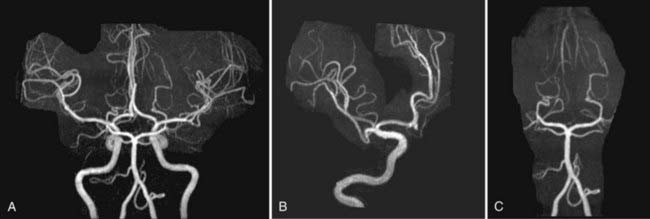
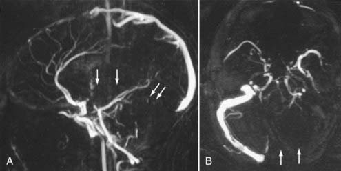
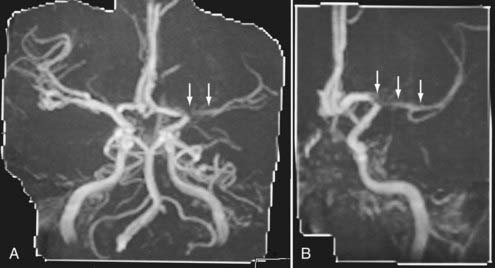
Nonemergency MR evaluation of patients with symptoms of intracranial or extracranial ischemic vascular disease usually begins with a routine brain MRI study that includes T2-weighted and FLAIR images for maximal sensitivity to detect subacute and chronic evidence of cerebral ischemic disease. MRA of the brain to evaluate the major intracranial arteries and their proximal branches is now a well-established technique. MRA typically uses a 3D TOF technique with added magnetization transfer pulse to improve the visualization of distal branches (Fig. 17-50). An MR venogram to exclude major venous thrombosis can be performed with either 3D TOF or phase-contrast techniques, which can easily identify the major superficial and deep venous sinuses and veins (Fig. 17-51). MRA has acceptable accuracy in evaluation of the intracranial internal carotid, vertebral, and basilar arteries, as well as the proximal branches of the anterior, middle, and posterior cerebral arteries in the setting of significant atherosclerotic stenoses, vasospasm, or vasculitis (Fig. 17-52).92 However, MRA is limited in its evaluation of medium-sized and small arteries. When such a disease process is clinically suspected and suggested by a routine MRI study (i.e., abnormal lesions on T2-weighted or FLAIR images), conventional angiography is often warranted. Evaluation of the carotid and vertebral arteries in the neck can be performed with 2D or 3D TOF or phase-contrast MR techniques without the use of intravenous gadolinium contrast. The accuracy of these techniques in comparison to conventional contrast-enhanced angiography is well described.93,94 A newer technique using a 3D spoiled gradient recalled (SPGR) pulse sequence obtained after rapid bolus intravenous injection of gadolinium can improve the accuracy of noninvasive MR vascular evaluation (Fig. 17-53).95 Similar to brain CTA, MRA is increasingly being used as an initial noninvasive imaging study for intracranial aneurysms or as a follow-up imaging study for untreated or treated intracranial aneurysms.95,96 MRA or CTA of a previously coiled or clipped aneurysm can be challenging because of inherent MR or CT artifacts generated by coils or clips. It is difficult to exclude a small recanalization or residual aneurysm on CTA because of a large amount of artifact from an aneurysm clip or coils. However, gadolinium bolus MRA of the brain may demonstrate recanalization of an intracranial aneurysm previously treated by endovascular coil embolization better than conventional TOF MRA without contrast enhancement (Fig. 17-54).97,98
Trauma
In acute CNS trauma, evaluation for a fracture or hemorrhage is still best done with a non–contrast-enhanced CT scan. However, because of its superior tissue contrast, MRI may better define small parenchymal abnormalities on T2-weighed, FLAIR, and gradient-recalled echo (GRE) images that may not be visible on CT. GRE is the most sensitive pulse sequence for acute/subacute blood breakdown products.99 MRI also appears to be superior to CT in evaluating posterior fossa pathology because the usual posterior fossa beam-hardening artifacts typically observed on CT are absent. MRI is also useful in the evaluation of small cortical contusions and subdural and epidural hematomas because of its higher tissue contrast and the ease of multiplanar acquisition with MRI. Small subacute SDHs, which are often isodense and therefore subtle on CT, are typically T1 and T2 hyperintense on MRI and thus more conspicuous. The MRI appearances of subdural and epidural hematomas and hygromas are variable and depend on the age and history (i.e., repeat hemorrhages). In the acute and subacute stages, T1 and T2 signal characteristics are similar to those observed with parenchymal hematomas. They are T1 isointense to hypointense and T2 hypointense in the acute stage because of intracellular deoxyhemoglobin and methemoglobin and become T1 hyperintense and T2 hyperintense in the subacute stage from extracellular methemoglobin. In the chronic stage, parenchymal hemorrhages are hypointense on T1- and markedly hypointense on T2-weighted images as a result of susceptibility effects from intracellular ferritin and hemosiderin, which are mostly present in the interstitium and within macrophages. However, chronic SDHs (hygromas) are T1 hypointense and T2 hyperintense in signal, similar to those of CSF. This reflects the low-density fluid collection that is typically observed on CT. Some authors suggest that MRI with a FLAIR pulse sequence has high sensitivity for acute SAH, but significant debate remains about its accuracy in the presence of frequently observed CSF flow–related artifacts associated with this pulse sequence, especially in the basal cisterns.100–102
MRI is especially helpful in the evaluation of patients with diffuse axonal injury (DAI), which usually results from a high-speed acceleration and deceleration injury that causes mechanical stress on the brain and thus results in “shear” injuries.103 The multiple, small and subtle shear injuries at the gray-white matter border, along the corpus callosum, and within the brainstem, typical of DAI, are much better evaluated with MRI than CT. The GRE pulse sequence, which is highly sensitive to areas of changes in susceptibility, is valuable when diffuse small parenchymal hemorrhages in the setting of trauma are evaluated. On T2-weighted and FLAIR images, these small superficial gray-white matter border lesions and deep pericallosal, deep gray matter, and upper brainstem lesions are hyperintense. If hemorrhagic, these lesions are also hypointense on GRE images because of changes in susceptibility associated with acute blood breakdown products such as deoxyhemoglobin and intracellular methemoglobin.104 In the chronic stage, hemosiderin and ferritin result in hypointensity on T2-weighted and GRE images.105
Brain MRI can be useful when a patient with an acute head injury has minimal CT abnormalities but has profound neurological deficits. In addition, MRI may be helpful when an objective measure of extensive brain injury, particularly brainstem injury, is required before a patient’s prognosis is discussed with the family. Newer MRI techniques such as DWI, perfusion MRI, and MRS may play additional roles in trauma patients to detect areas of ischemia and infarction.106
Vascular Malformations
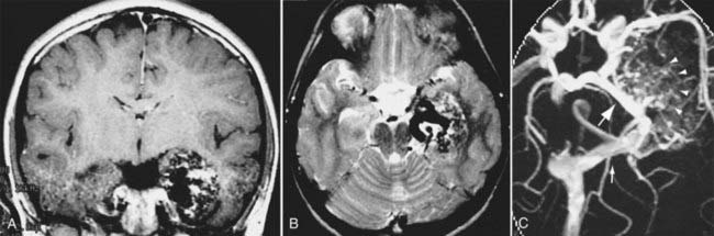
Intracerebral vascular malformations include four distinct types: AVM, cavernous malformation (cavernous angioma or hemangioma), developmental venous anomaly (DVA, previously known as venous malformation or venous angioma), and capillary telangiectasia. All except capillary telangiectasia are typically visible on MRI. An AVM is a vascular malformation that consists of a nidus that lacks the normal capillary network with ensuing direct communication between abnormally enlarged thick-walled feeding arterial channels and thin-walled draining venous channels. The vessels often lack normal smooth muscle and elastic lamina layers. AVMs may often be associated with aneurysms of feeding arteries or the draining veins (venous varix). There is no normal parenchyma intermixed with an AVM, although some gliosis may be observed. On MRI, an AVM appears as a complex tangle of abnormally enlarged vessels that demonstrate flow voids because of a high-flow state. Secondary findings such as subacute and chronic blood breakdown products (methemoglobin, ferritin, and hemosiderin) can be found with corresponding areas of T2 and GRE hypointensity.107 Similar small T2 hypointensity is also observed in the setting of calcifications associated with an AVM. Surrounding areas of edema, ischemia, or encephalomalacia may also be present.108 These areas are visible on T2-weighted and FLAIR images as hyperintensity with or without loss of volume in the case of chronic atrophy. Thin, linear cortical T1 hyperintensity may also be observed if cortical laminar necrosis from chronic ischemia as a result of a physiologic steal phenomenon occurs in the parenchyma adjacent to the AVM. AVMs can also be further visualized with 2D or 3D MRA using either phase-contrast or TOF techniques (Fig. 17-55).109 These MRI techniques can be used to diagnose AVMs and help in preoperative localization with 3D intraoperative guidance software. MRI is also useful in monitoring smaller AVMs treated by stereotactic radiosurgery (linear accelerator or Gamma Knife techniques).110,111
Cavernous malformations are slow-flow vascular malformations made up of abnormally large venous channels without associated abnormally enlarged feeding arteries or draining veins. They become symptomatic and also visible on MRI because they frequently bleed.112 Typically, cavernous malformations are discrete parenchymal masses with heterogeneous hypointensity and hyperintensity on T1- and T2-weighted images as a result of blood breakdown products of various ages. When recent hemorrhage is present, reactive T2 hyperintense surrounding edema may be seen with associated local mass effect.113 Multiple cavernous malformations are found in patients with vascular malformation syndromes. Because MRI, among all the imaging techniques, including conventional angiography, best visualizes these cavernous malformations, it is the study of choice in the initial evaluation and follow-up of patients with cavernomas (Fig. 17-56).
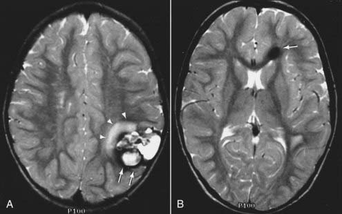
A DVA (as mentioned before, previously known as venous malformation or venous angioma) is not a pathologic vascular malformation. Instead, a DVA is a normal variant in which several prominent deep parenchymal veins drain a normal part of the brain and then drain into an unusually large superficial or deep draining vein. The angiographic and MRI appearance of these malformations has been described in the literature as resembling the “head of Medusa,” a Greek mythologic figure with a head of “hair” made of multiple live serpents. Because this is a benign entity and requires no intervention, its recognition on imaging studies is essential. DVAs have a typical imaging appearance on MRI that consists of several slightly prominent vessels with flow voids on T2-weighted images that drain into a larger draining vein.114 They are best visualized on contrast-enhanced T1-weighted images (Fig. 17-57). DVAs may sometimes coexist with cavernous malformations. If a hemorrhage is present in the vicinity of a DVA, the cause of hemorrhage is most likely an occult cavernous malformation neighboring the DVA.
Capillary telangiectasia is a histopathologic diagnosis rather than a radiologic one. It is rarely diagnosed preoperatively. If capillary telangiectasia is visible on MRI, it appears as a nonspecific focus of T2 hyperintensity, which may be associated with subtle enhancement on contrast-enhanced T1-weighted images. Multiple capillary telangiectases are found in patients with ataxia-telangiectasia syndrome, which affects both the CNS and other viscera.115
Seizure and Epilepsy
Several different MRI protocols have been developed over the years to evaluate epilepsy patients. These protocols usually include a type of high-resolution, 3D, and heavily T1-weighted acquisition of the whole brain. An SPGR sequence is one such pulse sequence that can be obtained at 1-mm intervals in the axial, coronal, and sagittal planes. Small slice thickness along with its heavily T1-weighted parameters accentuates the signal difference between gray and white matter and thus improves the detection of small focal heterotopias and migration anomalies.116,117 MRI acquisition with the use of phased-array surface coils over a part of the head instead of the usual head coil used for brain MRI may also improve resolution and sensitivity. These surface coils have an improved signal-to-noise ratio that is usually severalfold greater than that obtained with a routine head coil and have the flexibility to be placed directly over the part of the brain that is suspected of containing the epileptic focus. They are useful in the evaluation of small cortical or subcortical lesions, which may not otherwise be visible on routine brain MRI. The advantages of surface coils diminish for deeper structures because the signal decreases as the distance between the coil and the structure increases. Nonetheless, phased-array surface coils have been used successfully to evaluate the mesial temporal lobes in patients with complex partial seizures referable to the temporal lobes. In many of these patients, MRI correlates of mesial temporal sclerosis, such as hippocampal atrophy, abnormal T2 hippocampal hyperintensity, and disruption of the hippocampal internal architecture, are observed.118–120 Such imaging of the mesial temporal lobes is best done in a coronal or modified coronal plane perpendicular to the anteroposterior axis of the hippocampus at 1- to 20-mm intervals using T1, T2, and FLAIR images (Fig. 17-58).
Tailored MRI techniques are valuable in the preoperative imaging evaluation of epileptic patients. In particular, these techniques are useful in the preoperative evaluation and lateralization of the seizure focus in patients with temporal lobe epilepsy. Various MRI parameters can be used to diagnose the presence of mesial temporal sclerosis in patients with temporal lobe epilepsy, including qualitative techniques such as visual evaluation for asymmetrically and abnormally increased signal on T2 and FLAIR coronal images, decreased hippocampal volume, and larger than normal size of the temporal horn of the lateral ventricle within the ipsilateral temporal lobe. Quantitative measurements of these changes can be studied with 3D hippocampal volumetry to quantify the hippocampal atrophy and T2 relaxometry to quantify the change in T2 signal. Such MRI lateralization, when possible, has significant prognostic value for patients who undergo surgery to treat medically intractable temporal lobe epilepsy. Patients with a lateralizing MRI abnormality have a significantly greater seizure-free rate after hippocampal resection and partial temporal lobectomy than do those who do not demonstrate such a lateralizing abnormality on preoperative MRI.121,122 MRS can also be used to study the mesial temporal lobes, including the hippocampus, in temporal lobe epilepsy. Single-voxel and 2D chemical shift imaging techniques are used to obtain proton MR spectra from the hippocampi and surrounding mesial temporal lobe structures. In MRS, neuronal concentration and integrity are ascertained by measuring the concentration of the neuronal marker metabolite NAA with an absolute quantitative technique or, more commonly, by a ratio that compares NAA with a reference metabolite such as creatine. A high accuracy rate in lateralization of the diseased hippocampus in patients with temporal lobe epilepsy is reported with the use of single-voxel or chemical shift imaging proton MRS.47,123–125
More recently, activation fMRI and diffusion tensor imaging with 2D and 3D white matter tractography are also being used as a part of preoperative evaluation and surgical planning for patients with epilepsy, especially temporal lobe epilepsy. Molecular imaging using single-photon emission CT (SPECT)- and PET-visible receptor ligands can also help localize areas of cortical malformations and epileptogenic foci.126–129
Aine CJ. A conceptual overview and critique of functional neuroimaging techniques in humans: I. MRI/fMRI and PET. Crit Rev Neurobiol. 1995;9:229-309.
Bradley WG, Shey RB. MR imaging evaluation of seizures. Radiology. 2000;214:651-656.
Burdette JH, Elster AD, Ricci PE. Acute cerebral infarction: quantification of spin-density and T2 shine-through phenomena on diffusion-weighted MR images. Radiology. 1999;212:333-339.
Falcone S, Post MJ. Encephalitis, cerebritis, and brain abscess: pathophysiology and imaging findings. Neuroimaging Clin N Am. 2000;10:333-353.
Gentry LR. Imaging of closed head injury. Radiology. 1994;191:1-17.
Hounsfield GN. Computerized transverse axial scanning (tomography). 1. Description of system. Br J Radiol. 1973;46:1016-1022.
Huda W. Review of Radiologic Physics, 3rd ed. Baltimore: Lippincott Williams & Wilkins; 2009.
Jack CRJr. Magnetic resonance imaging. Neuroimaging and anatomy. Neuroimaging Clin N Am. 1995;5:597-622.
Lev MH, Rosen BR. Clinical applications of intracranial perfusion MR imaging. Neuroimaging Clin N Am. 1999;9:309-331.
Luat AF, Chugani HT. Molecular and diffusion tensor imaging of epileptic networks. Epilepsia. 2008;49(suppl 3):15-22.
McLean MA, Cross JJ. Magnetic resonance spectroscopy: principles and applications in neurosurgery. Br J Neurosurg. 2009;23:5-13.
Okahara M, Kiyosue H, Yamashita M, et al. Diagnostic accuracy of magnetic resonance angiography for cerebral aneurysms in correlation with 3D-digital subtraction angiographic images: a study of 133 aneurysms. Stroke. 2002;33:1803-1808.
Okazaki H. Fundamentals of Neuropathology: Morphologic Basis of Neurologic Disorders, 2nd ed. New York: Igaku-Shoin; 1989.
Osborne A. Diagnostic Neuroradiology. St. Louis: CV Mosby; 1994.
Ricci PE. Imaging of adult brain tumors. Neuroimaging Clin N Am. 1999;9:651-669.
Ross B, Michaelis T. Clinical applications of magnetic resonance spectroscopy. Magn Reson Q. 1994;10:191-247.
Rowley HA, Grant PE, Roberts TP. Diffusion MR imaging. Theory and applications. Neuroimaging Clin N Am. 1999;9:343-361.
Sorensen AG, Copen WA, Ostergaard L, et al. Hyperacute stroke: simultaneous measurement of relative cerebral blood volume, relative cerebral blood flow, and mean tissue transit time. Radiology. 1999;2102:519-527.
Wikström J, Ronne-Engström E, Gal G, et al. Three-dimensional time-of-flight (3D TOF) magnetic resonance angiography (MRA) and contrast-enhanced MRA of intracranial aneurysms treated with platinum coils. Acta Radiol. 2008;49:190-196.
Wintermark M, Dillon WP, Smith WS, et al. Visual grading system for vasospasm based on perfusion CT imaging: comparisons with conventional angiography and quantitative perfusion CT. Cerebrovasc Dis. 2008;26:163-170.
Wintermark M, Sincic R, Sridhar D, et al. Cerebral perfusion CT: technique and clinical applications. J Neuroradiol. 2008;35:253-260.
Woermann FG, Vollmar C. Clinical MRI in children and adults with focal epilepsy: a critical review. Epilepsy Behav. 2009;15:40-49.
Yetkin FZ, Mueller WM, Morris GL, et al. Functional MR activation correlated with intraoperative cortical mapping. AJNR Am J Neuroradiol. 1997;18:1311-1315.
1 Hounsfield GN. Computerized transverse axial scanning (tomography). 1. Description of system. Br J Radiol. 1973;462:1016-1022.
2 Freemon FR, Allen JH, Duncan GW, et al. Controlled use of cranial computerized tomography. Arch Neurol. 1978;35:129-132.
3 Huda W. Review of Radiologic Physics, 3rd ed. Baltimore: Lippincott Williams & Wilkins; 2009.
4 Mahesh M. Search for isotropic resolution in CT from conventional through multiple-row detector. Radiographics. 2002;22:949-962.
5 Naidich TP, Lin JP, Leeds NE, et al. Primary tumors and other masses of the cerebellum and fourth ventricle: differential diagnosis by computed tomography. Neuroradiology. 1977;14:153-174.
6 Koo AH, LaRoque RL. Evaluation of head trauma by computed tomography. Radiology. 1977;123:345-350.
7 Liliequist B, Lindqvist M, Valdimarsson E. Computed tomography and subarachnoid hemorrhage. Neuroradiology. 1977;14:21-26.
8 Lin JP, Pay N, Naidich TP, et al. Computed tomography in the postoperative care of neurosurgical patients. Neuroradiology. 1977;12:185-189.
9 Hryshko FG, Deeb ZL. Computed tomography in acute head injuries. J Comput Tomogr. 1983;7:331-344.
10 Merino-deVillasante J, Taveras JM. Computerized tomography (CT) in acute head trauma. AJR Am J Roentgenol. 1976;126:765-778.
11 Fitz CR, Harwood-Nash DC. Computed tomography in hydrocephalus. J Comput Tomogr. 1978;2:91-108.
12 Harden SP, Dey C, Gawne-Cain ML. Cranial CT of the unconscious adult patient. Clin Radiol. 2007;62:404-415.
13 Chappell ET, Moure FC, Good MC. Comparison of computed tomographic angiography with digital subtraction angiography in the diagnosis of cerebral aneurysms: a meta-analysis. Neurosurgery. 2003;52:624-631.
14 Dammert S, Krings T, Moller-Hartmann W, et al. Detection of intracranial aneurysms with multislice CT: comparison with conventional angiography. Neuroradiology. 2004;46:427-434.
15 Bub LD, Hollingworth W, Jarvik JG, et al. Screening for blunt cerebrovascular injury: evaluating the accuracy of multidetector computed tomographic angiography. J Trauma. 2005;59:691-697.
16 Wintermark M, Sincic R, Sridhar D, et al. Cerebral perfusion CT: technique and clinical applications. J Neuroradiol. 2008;35:253-260.
17 Wintermark M, Thiran JP, Maeder P, et al. Simultaneous measurement of regional cerebral blood flow by perfusion CT and stable xenon CT: a validation study. AJNR Am J Neuroradiol. 2001;22:905-914.
18 Kamath A, Smith WS, Powers WJ, et al. Perfusion CT compared to H(2) (15)O/O (15)O PET in patients with chronic cervical carotid artery occlusion. Neuroradiology. 2008;50:745-751.
19 Nogueira RG, Lev MH, Roccatagliata L, et al. Intra-arterial nicardipine infusion improves CT perfusion–measured cerebral blood flow in patients with subarachnoid hemorrhage-induced vasospasm. AJNR Am J Neuroradiol. 2009;30:160-164.
20 Laslo AM, Eastwood JD, Pakkiri P, et al. CT perfusion–derived mean transit time predicts early mortality and delayed vasospasm after experimental subarachnoid hemorrhage. AJNR Am J Neuroradiol. 2008;29:79-85.
21 Wintermark M, Dillon WP, Smith WS, et al. Visual grading system for vasospasm based on perfusion CT imaging: comparisons with conventional angiography and quantitative perfusion CT. Cerebrovasc Dis. 2008;26:163-170.
22 Bloch F, Hansen W, Packard M. The nuclear induction experiment. Phys Rev. 1946;70:474-485.
23 Purcell EM, Hansen WW, Packard ME. Resonance absorption by nuclear magnetic moments in a solid. Phys Rev. 1946;69:37-38.
24 Bloembergen N, Purcell EM, Pound RV. Relaxation effects in nuclear magnetic resonance absorption. Phys Rev. 1948;73:679-712.
25 Slichter CP. Principles of Magnetic Resonance, 2nd ed. Berlin: Springer-Verlag; 1978.
26 Rabi II, Millman S, Kusch P, et al. The molecular beam resonance method for measuring nuclear magnetic moments—the magnetic moments of li-3(6) li-3(7) and f-9(19). Phys Rev. 1939;55:526-535.
27 Hahn EL. Spin echoes. Phys Rev. 1950;80:580-594.
28 Wolf GL, Burnett KR, Goldstein EJ, et al. Contrast agents for magnetic resonance imaging. Magn Reson Annu. 1985:231-266.
29 Turner R, Le Bihan D, Chesnick AS. Echo-planar imaging of diffusion and perfusion. Magn Reson Med. 1991;19:247-253.
30 Donahue KM, Weisskoff RM, Chesler DA, et al. Improving MR quantification of regional blood volume with intravascular T1 contrast agents: accuracy, precision, and water exchange. Magn Reson Med. 1996;36:858-867.
31 Melki PS, Jolesz FA, Mulkern RV. Partial RF echo planar imaging with the FAISE method. I. Experimental and theoretical assessment of artifact. Magn Reson Med. 1992;26:328-341.
32 De Coene B, Hajnal JV, Gatehouse P, et al. MR of the brain using fluid-attenuated inversion recovery (FLAIR) pulse sequences. AJNR Am J Neuroradiol. 1992;13:1555-1564.
33 Mansfield P. Real-time echo-planar imaging by NMR. Br Med Bull. 1984;40:187-190.
34 Pierpaoli C, Righini A, Linfante I, et al. Histopathologic correlates of abnormal water diffusion in cerebral ischemia: diffusion-weighted MR imaging and light and electron microscopic study. Radiology. 1993;189:439-448.
35 Wong EC, Buxton RB, Frank LR. Quantitative imaging of perfusion using a single subtraction (QUIPSS and QUIPSS II). Magn Reson Med. 1998;39:702-708.
36 Soares DP, Law M. Magnetic resonance spectroscopy of the brain: review of metabolites and clinical applications. Clin Radiol. 2009;64:12-21.
37 McLean MA, Cross JJ. Magnetic resonance spectroscopy: principles and applications in neurosurgery. Br J Neurosurg. 2009;23:5-13.
38 Ogawa S, Lee TM, Kay AR, et al. Brain magnetic resonance imaging with contrast dependent on blood oxygenation. Proc Natl Acad Sci U S A. 1990;87:9868-9872.
39 Aine CJ. A conceptual overview and critique of functional neuroimaging techniques in humans: I. MRI/fMRI and PET. Crit Rev Neurobiol. 1995;9:229-309.
40 Okazaki H. Fundamentals of Neuropathology: Morphologic Basis of Neurologic Disorders, 2nd ed. New York: Igaku-Shoin; 1989.
41 Mascalchi M, Muscas GC, Galli C, et al. MRI of pleomorphic xanthoastrocytoma: case report. Neuroradiology. 1994;36:446-447.
42 Ricci PE. Imaging of adult brain tumors. Neuroimaging Clin N Am. 1999;9:651-669.
43 Watanabe M, Tanaka R, Takeda N. Magnetic resonance imaging and histopathology of cerebral gliomas. Neuroradiology. 1992;34:463-469.
44 Khatib ZA, Heideman RL, Kovnar EH, et al. Predominance of pilocytic histology in dorsally exophytic brain stem tumors. Pediatr Neurosurg. 1994;20:2-10.
45 Sun B, Wang CC, Wang J. MRI characteristics of midbrain tumours. Neuroradiology. 1999;41:158-162.
46 Graif M, Bydder GM, Steiner RE, et al. Contrast-enhanced MR imaging of malignant brain tumors. AJNR Am J Neuroradiol. 1985;6:855-862.
47 Ross B, Bluml S. Magnetic resonance spectroscopy of the human brain. Anat Rec. 2001;265:54-84.
48 Ross B, Michaelis T. Clinical applications of magnetic resonance spectroscopy. Magn Reson Q. 1994;10:191-247.
49 Tzika AA, Vigneron DB, Dunn RS, et al. Intracranial tumors in children: small single-voxel proton MR spectroscopy using short- and long-echo sequences. Neuroradiology. 1996;38:254-263.
50 Achten E, Jackson GD, Cameron JA, et al. Presurgical evaluation of the motor hand area with functional MR imaging in patients with tumors and dysplastic lesions. Radiology. 1999;210:529-538.
51 Aronen HJ, Gazit IE, Louis DN, et al. Cerebral blood volume maps of gliomas: comparison with tumor grade and histologic findings. Radiology. 1994;191:41-51.
52 Yetkin FZ, Mueller WM, Morris GL, et al. Functional MR activation correlated with intraoperative cortical mapping. AJNR Am J Neuroradiol. 1997;18:1311-1315.
53 Yetkin FZ, Papke RA, Mark LP, et al. Location of the sensorimotor cortex: functional and conventional MR compared. AJNR Am J Neuroradiol. 1995;16:2109-2113.
54 Lee YY, Van Tassel P. Intracranial oligodendrogliomas: imaging findings in 35 untreated cases. AJR Am J Roentgenol. 1989;152:361-369.
55 Spoto GP, Press GA, Hesselink JR, et al. Intracranial ependymoma and subependymoma: MR manifestations. AJNR Am J Neuroradiol. 1990;11:83-91.
56 Coates TL, Hinshaw DBJr, Peckman N, et al. Pediatric choroid plexus neoplasms: MR, CT, and pathologic correlation. Radiology. 1989;173:81-88.
57 Spagnoli MV, Goldberg HI, Grossman RI, et al. Intracranial meningiomas: high-field MR imaging. Radiology. 1986;161:369-375.
58 Elster AD, Challa VR, Gilbert TH, et al. Meningiomas: MR and histopathologic features. Radiology. 1989;170:857-862.
59 Fujii K, Fujita N, Hirabuki N, et al. Neuromas and meningiomas: evaluation of early enhancement with dynamic MR imaging. AJNR Am J Neuroradiol. 1992;13:1215-1220.
60 Wilms G, Lammens M, Marchal G, et al. Prominent dural enhancement adjacent to nonmeningiomatous malignant lesions on contrast-enhanced MR images. AJNR Am J Neuroradiol. 1991;12:761-764.
61 Tokumaru A, O’uchi T, Eguchi T, et al. Prominent meningeal enhancement adjacent to meningioma on Gd-DTPA–enhanced MR images: histopathologic correlation. Radiology. 1990;175:431-433.
62 Dwyer AJ, Frank JA, Doppman JL, et al. Pituitary adenomas in patients with Cushing disease: initial experience with Gd-DTPA–enhanced MR imaging. Radiology. 1987;1632:421-426.
63 Simonetta AB. Imaging of suprasellar and parasellar tumors. Neuroimaging Clin N Am. 1999;9:717-732.
64 Healy ME, Hesselink JR, Press GA, et al. Increased detection of intracranial metastases with intravenous Gd-DTPA. Radiology. 1987;165:619-624.
65 Potts DG, Abbott GF, von Sneidern JV. National Cancer Institute study: evaluation of computed tomography in the diagnosis of intracranial neoplasms. III. Metastatic tumors. Radiology. 1980;136:657-664.
66 Sze G, Soletsky S, Bronen R, et al. MR imaging of the cranial meninges with emphasis on contrast enhancement and meningeal carcinomatosis. AJR Am J Roentgenol. 1989;153:1039-1049.
67 Bilaniuk LT. Adult infratentorial tumors. Semin Roentgenol. 1990;25:155-173.
68 Osborne A, Rausching W. Brain tumors and tumorlike masses: classification and differential diagnosis. Diagnostic Neuroradiology. St. Louis: CV Mosby, 1994;437-442.
69 Osborne A, Rausching W. Brain tumors and tumorlike masses: classification and differential diagnosis. Diagnostic Neuroradiology. St. Louis: CV Mosby, 1994;446-448.
70 Osborne A, Rausching W. Brain tumors and tumorlike masses: classification and differential diagnosis. Diagnostic Neuroradiology. St. Louis: CV Mosby, 1994;435-436.
71 Chang KH, Han MH, Roh JK, et al. Gd-DTPA–enhanced MR imaging of the brain in patients with meningitis: comparison with CT. AJR Am J Roentgenol. 1990;154:809-816.
72 Lizerbram EK, Hesselink JR. Neuroimaging of AIDS. I. Viral infections. Neuroimaging Clin N Am. 1997;7:261-280.
73 Foerster BR, Thurnher MM, Malani PN, et al. Intracranial infections: clinical and imaging characteristics. Acta Radiol. 2007;48:875-893.
74 Falcone S, Post MJ. Encephalitis, cerebritis, and brain abscess: pathophysiology and imaging findings. Neuroimaging Clin N Am. 2000;10:333-353.
75 Chang L, Ernst T. MR spectroscopy and diffusion-weighted MR imaging in focal brain lesions in AIDS. Neuroimaging Clin N Am. 1997;7:409-426.
76 Kim YJ, Chang KH, Song IC, et al. Brain abscess and necrotic or cystic brain tumor: discrimination with signal intensity on diffusion-weighted MR imaging. AJR Am J Roentgenol. 1998;171:1487-1490.
77 Whiteman ML. Neuroimaging of central nervous system tuberculosis in HIV-infected patients. Neuroimaging Clin N Am. 1997:7199-7214.
78 Goyal M, Sharma A, Mishra NK, et al. Imaging appearance of pachymeningeal tuberculosis. AJR Am J Roentgenol. 1997;169:1421-1424.
79 Shah GV. Central nervous system tuberculosis: imaging manifestations. Neuroimaging Clin N Am. 2000;10:355-374.
80 Go JL, Kim PE, Ahmadi J, et al. Fungal infections of the central nervous system. Neuroimaging Clin N Am. 2000;10:409-425.
81 Delone DR, Goldstein RA, Petermann MS, et al. Disseminated aspergillosis involving the brain: distribution and imaging characteristics. AJNR Am J Neuroradiol. 1999;20:1597-1604.
82 Del Brutto OH, Zenteno MA, Salgado P, et al. MR imaging in cysticercotic encephalitis. AJNR Am J Neuroradiol. 1989;10(5 suppl):S18-S20.
83 Noujaim SE, Rossi MD, Rao SK, et al. CT and MR imaging of neurocysticercosis. AJR Am J Roentgenol. 1999;173:1485-1490.
84 Rowley HA, Grant PE, Roberts TP. Diffusion MR imaging. Theory and applications. Neuroimaging Clin N Am. 1999;9:343-361.
85 Chien D, Kwong KK, Gress DR, et al. MR diffusion imaging of cerebral infarction in humans. AJNR Am J Neuroradiol. 1992;13:1097-1102.
86 Gonzalez RG, Schaefer PW, Buonanno FS, et al. Diffusion-weighted MR imaging: diagnostic accuracy in patients imaged within 6 hours of stroke symptom onset. Radiology. 1999;210:155-162.
87 Burdette JH, Elster AD, Ricci PE. Acute cerebral infarction: quantification of spin-density and T2 shine-through phenomena on diffusion-weighted MR images. Radiology. 1999;212:333-339.
88 Sorensen AG, Copen WA, Ostergaard L, et al. Hyperacute stroke: simultaneous measurement of relative cerebral blood volume, relative cerebral blood flow, and mean tissue transit time. Radiology. 1999;210:519-527.
89 Lev MH, Rosen BR. Clinical applications of intracranial perfusion MR imaging. Neuroimaging Clin N Am. 1999;9:309-331.
90 Gillard JH, Barker PB, van Zijl PC, et al. Proton MR spectroscopy in acute middle cerebral artery stroke. AJNR Am J Neuroradiol. 1996;17:873-886.
91 Holshouser BA, Ashwal S, Luh GY, et al. Proton MR spectroscopy after acute central nervous system injury: outcome prediction in neonates, infants, and children. Radiology. 1997;202:487-496.
92 Knopp EA. The role of magnetic resonance angiography in the assessment of intracranial vascular disease. Neuroimaging Clin North Am. 1996;6:769-780.
93 Bernstein MA, Huston J3rd, Lin C, et al. High-resolution intracranial and cervical MRA at 3.0T: technical considerations and initial experience. Magn Reson Med. 2001;46(5):955-962.
94 Okahara M, Kiyosue H, Yamashita M, et al. Diagnostic accuracy of magnetic resonance angiography for cerebral aneurysms in correlation with 3D-digital subtraction angiographic images: a study of 133 aneurysms. Stroke. 2002;33:1803-1808.
95 Metens T, Rio F, Balériaux D, et al. Intracranial aneurysms: detection with gadolinium-enhanced dynamic three-dimensional MR angiography—initial results. Radiology. 2000;216:39-46.
96 Kouskouras C, Charitanti A, Giavroglou C, et al. Intracranial aneurysms: evaluation using CTA and MRA. Correlation with DSA and intraoperative findings. Neuroradiology. 2004;46:842-850.
97 Wikström J, Ronne-Engström E, Gal G, et al. Three-dimensional time-of-flight (3D TOF) magnetic resonance angiography (MRA) and contrast-enhanced MRA of intracranial aneurysms treated with platinum coils. Acta Radiol. 2008;49:190-196.
98 Farb RI, Nag S, Scott JN, et al. Surveillance of intracranial aneurysms treated with detachable coils: a comparison of MRA techniques. Neuroradiology. 2005;47:507-515.
99 Gentry LR. Imaging of closed head injury. Radiology. 1994;191:1-17.
100 Singer MB, Atlas SW, Drayer BP. Subarachnoid space disease: diagnosis with fluid-attenuated inversion-recovery MR imaging and comparison with gadolinium-enhanced spin-echo MR imaging—blinded reader study. Radiology. 1998;208:417-422.
101 Noguchi K, Seto H, Kamisaki Y, et al. Comparison of fluid-attenuated inversion-recovery MR imaging with CT in a simulated model of acute subarachnoid hemorrhage. AJNR Am J Neuroradiol. 2000;21:923-927.
102 Ashikaga R, Araki Y, Ishida O. MRI of head injury using FLAIR. Neuroradiology. 1997;39:239-242.
103 Le TH, Gean AD. Neuroimaging of traumatic brain injury. Mt Sinai J Med. 2009;76:145-162.
104 Sehgal V, Delproposto Z, Haacke EM, et al. Clinical applications of neuroimaging with susceptibility-weighted imaging. J Magn Reson Imaging. 2005;22:439-450.
105 Morioka T, Nishio S, Mihara F, et al. Usefulness of T2* weighted magnetic resonance image in the diagnosis of head injury on chronic stage. No To Shinkei. 1999;51:703-708.
106 Ross BD, Ernst T, Kreis R, et al. 1H MRS in acute traumatic brain injury. J Magn Reson Imaging. 1998;8:829-840.
107 Saleh RS, Singhal A, Lohan D, et al. Assessment of cerebral arteriovenous malformations with high temporal and spatial resolution contrast-enhanced magnetic resonance angiography: a review from protocol to clinical application. Top Magn Reson Imaging. 2008;19:251-257.
108 Nussel F, Wegmuller H, Huber P. Comparison of magnetic resonance angiography, magnetic resonance imaging and conventional angiography in cerebral arteriovenous malformation. Neuroradiology. 1991;33:56-61.
109 Huston J3rd, Rufenacht DA, Ehman RL, et al. Intracranial aneurysms and vascular malformations: comparison of time-of-flight and phase-contrast MR angiography. Radiology. 1991;181:721-730.
110 Marks MP, Delapaz RL, Fabrikant JI, et al. Intracranial vascular malformations: imaging of charged-particle radiosurgery. Part I. Results of therapy. Radiology. 1988;168:447-455.
111 Marks MP, Delapaz RL, Fabrikant JI, et al. Intracranial vascular malformations: imaging of charged-particle radiosurgery. Radiology. 1988;168:457-462.
112 Porter PJ, Willinsky RA, Harper W, et al. Cerebral cavernous malformations: natural history and prognosis after clinical deterioration with or without hemorrhage. J Neurosurg. 1997;87:190-197.
113 Rigamonti D, Drayer BP, Johnson PC, et al. The MRI appearance of cavernous malformations (angiomas). J Neurosurg. 1987;67:518-524.
114 Rigamonti D, Spetzler RF, Drayer BP, et al. Appearance of venous malformations on magnetic resonance imaging. J Neurosurg. 1988;69:535-539.
115 Lee RR, Becher MW, Benson ML, et al. Brain capillary telangiectasis: MR imaging appearance and clinicohistopathologic findings. Radiology. 1997;205:797-805.
116 Lehéricy S, Semah F, Hasboun D, et al. Temporal lobe epilepsy with varying severity: MRI study of 222 patients. Neuroradiology. 1997;39:788-796.
117 Jack CRJr. Magnetic resonance imaging. Neuroimaging and anatomy. Neuroimaging Clin N Am. 1995;5:597-622.
118 Barkovich AJ, Rowley HA, Andermann F. MR in partial epilepsy: value of high-resolution volumetric techniques. AJNR Am J Neuroradiol. 1995;16:339-343.
119 Bradley WG, Shey RB. MR imaging evaluation of seizures. Radiology. 2000;214:651-656.
120 Bronen RA, Cheung G, Charles JT, et al. Imaging findings in hippocampal sclerosis: correlation with pathology. AJNR Am J Neuroradiol. 1991;12:933-940.
121 Jack CRJr, Sharbrough FW, Twomey CK, et al. Temporal lobe seizures: lateralization with MR volume measurements of the hippocampal formation. Radiology. 1990;175:423-429.
122 Grant PE, Barkovich AJ, Wald LL, et al. High-resolution surface-coil MR of cortical lesions in medically refractory epilepsy: a prospective study. AJNR Am J Neuroradiol. 1997;18:291-301.
123 Ende GR, Laxer KD, Knowlton RC, et al. Temporal lobe epilepsy: bilateral hippocampal metabolite changes revealed at proton MR spectroscopic imaging. Radiology. 1997;202:809-817.
124 Hsu Y-Y, Chang C, Chang C-N, et al. Proton MR spectroscopy in patients with complex partial seizures: single-voxel spectroscopy versus chemical-shift imaging. AJNR Am J Neuroradiol. 1999;20:643-651.
125 Hajek M, Dezortova M, Krsek P. (1)H MR spectroscopy in epilepsy. Eur J Radiol. 2008;672:258-267.
126 Duncan J. The current status of neuroimaging for epilepsy. Curr Opin Neurol. 2009;22:179-184.
127 la Fougère C, Rominger A, Förster S, et al. PET and SPECT in epilepsy: a critical review. Epilepsy Behav. 2009;15:50-55.
128 Woermann FG, Vollmar C. Clinical MRI in children and adults with focal epilepsy: a critical review. Epilepsy Behav. 2009;15:40-49.
129 Luat AF, Chugani HT. Molecular and diffusion tensor imaging of epileptic networks. Epilepsia. 2008;49(suppl 3):15-22.