[level-membership-for-hematology-oncology-and-palliative-medicine-category]
Chapter 1 Biologic Basis of Radiation Oncology
What Is Radiation Biology?
Most of this chapter will be devoted to so-called classical radiobiology, that is, studies that largely predate the revolution in molecular biology of the 1980s and 1990s. Although the reader might be tempted to view this body of knowledge as rather primitive by today’s standards, relying too heavily on phenomenology, empiricism, and simplistic, descriptive models and theories, the real challenge is to integrate the new biology into the already-existing framework of classical radiobiology; this will be discussed in detail in Chapter 2.
Radiotherapy-Oriented Radiobiology: A Conceptual Framework
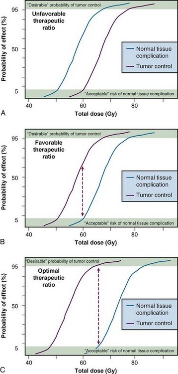
Therapeutic Ratio
The concept of therapeutic ratio is best illustrated graphically, by making a direct comparison of dose-response curves for both tumor control and normal tissue complication rates plotted as a function of dose. Examples of this approach are shown in Figure 1-1, for cases in which the therapeutic ratio is either “unfavorable,” “favorable,” or “optimal,” bearing in mind that these are theoretical curves. Actual dose-response curves derived from experimental or clinical data are much more variable, particularly for tumors, which tend to show much shallower dose responses.1 This serves to underscore how difficult it can be in practice to assign a single numerical value to the therapeutic ratio in any given situation.
Radiation Biology “Continuum”
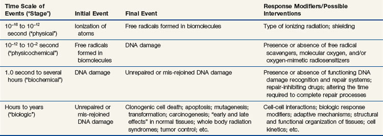
There is a surprising continuity between the physical events that occur in the first picosecond (or less) after ionizing radiation interacts with biologic material and the ultimate consequences of that interaction on tissues. The consequences themselves may not become apparent until days, weeks, months, or even years after the radiation exposure. Some of the important steps in this radiobiology “continuum” are listed in Table 1-1. The orderly progression from one stage of the continuum to the next—from physical to physicochemical to biochemical to biologic—is particularly noteworthy not only because of the vastly different time scales over which the critical events occur, but also because of the increasing biologic complexity associated with each of the endpoints or outcomes. Each stage of the continuum also offers a unique radiobiologic window of opportunity: the potential to intervene in the process and thereby modify all the events and outcomes that follow.
Tissue Heterogeneity
Normal tissues, being composed of more than one type of cell, are somewhat heterogeneous, and tumors, owing both to the genetic instability of individual tumor cells and to microenvironmental differences, are very heterogeneous. Different subpopulations of cells have been isolated from many types of human and experimental cancers, and these may differ in antigenicity, metastatic potential, sensitivity to radiation therapy and chemotherapy, and so on.2,3 This heterogeneity is manifest within a particular patient, and to a much greater extent, between patients with otherwise similar tumors.
What are the practical implications of normal tissue and tumor heterogeneity? First, if one assumes that normal tissues are the more uniform and predictable in behavior of the two, then tumor heterogeneity is responsible, either directly or indirectly, for most radiotherapy failures. If so, this suggests that a valid clinical strategy might be to identify the radioresistant subpopulation(s) of tumor cells and then tailor therapy specifically to cope with them. This approach is much easier said than done. Some prospective clinical studies now include one or more pretreatment determinations of, for example, the extent of tumor hypoxia4 or the potential doubling time of tumor clonogens5 as criteria for assigning patients to different treatment groups.
“Powers of Ten”
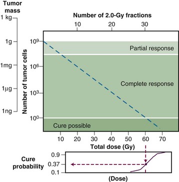
The tumor control probability for a given fraction of surviving cells is not particularly helpful if the total number of cells at risk is unknown, however, and this is where an understanding of logarithmic relationships and exponential cell killing is useful. Based on the resolution of existing tools and technology for cancer detection, let us assume that a 1-cm3 (1-g) tumor mass can be identified reliably. A tumor of this size has been estimated to contain approximately 109 cells,6 admittedly a theoretical value that assumes all cells are perfectly “packed” and uniformly sized and that the tumor contains no stroma. A further assumption, that all such cells are clonogenic (rarely, if ever, the case), suggests that at least 9 logs of cell killing would be necessary before any appreciable tumor control (about 37%) would be achieved, and 10 logs of cell killing would be required for a high degree of tumor control (i.e., 90%).
After the first log or two of cell killing, however, some tumors respond by shrinking, a partial response. After two to three logs of cell killing, the tumor may shrink to a size below the current limits of clinical detection, that is, a complete response. Although partial and complete responses are valid clinical endpoints, a complete response does not necessarily mean tumor cure. At least six more logs of cell killing would be required before any significant probability of cure would be expected. This explains why radiation therapy is not halted if the tumor “disappears” during the course of treatment; this concept is illustrated graphically in Figure 1-2.
Radiation Biology and Therapy: The First 50 Years
In less than 4 years after the discovery of x rays by Roentgen,7 radioactivity by Becquerel,8 and radium by the Curies,9 the new modality of cancer treatment known as radiation therapy claimed its first apparent cure of skin cancer.10 Today, more than a century later, radiotherapy is most commonly given as a series of small daily dose fractions of approximately 1.8 to 2 Gy each, 5 days per week, over a period of 5 to 7 weeks, to a total dose of 50 to 70 Gy. Although it is true that the historical development of this conventional radiotherapy schedule was empirically based, there were a number of early radiobiologic experiments that suggested this approach.
In the earliest days of radiotherapy, both x rays and radium were used for cancer treatment. Because of the greater availability and convenience of using x-ray tubes and the higher intensities of radiation output achievable, it was fairly easy to deliver large single doses in short overall treatment times. Thus, from about 1900 into the 1920s, this “massive dose technique”11 was a common way of administering radiation therapy. Unfortunately, normal tissue complications were quite severe. To make matters worse, the rate of local tumor recurrence was still unacceptably high.
As early as 1906, Bergonié and Tribondeau12 observed histologically that the immature dividing cells of the rat testis showed evidence of damage at lower radiation doses than the mature nondividing cells. Based on these observations, the two researchers put forth some basic “laws” stating that x rays were more effective on cells that were: (1) actively dividing, (2) likely to continue to divide indefinitely, and (3) poorly differentiated.12 Because tumors were already known to contain cells that not only were less differentiated but also exhibited greater mitotic activity, Bergonié and Tribondeau reasoned that several radiation exposures might preferentially kill these tumor cells but not their slowly proliferating, differentiated counterparts in the surrounding normal tissues.
The end of common usage of the single-dose technique in favor of fractionated treatment came during the 1920s as a consequence of the pioneering experiments of Claude Regaud and colleagues.13 Using the testis of the rabbit as a model tumor system (because the rapid and unlimited proliferation of spermatogenic cells simulated to some extent the pattern of cell proliferation in malignant tumors), Regaud14 showed that only through the use of multiple radiation exposures could animals be completely sterilized without producing severe injury to the scrotum. Regaud15 suggested that the superior results afforded the multifraction irradiation scheme were related to alternating periods of relative radioresistance and sensitivity in the rapidly proliferating germ cells. These principles were soon tested in the clinic by Henri Coutard,16,17 who used fractionated radiotherapy for the treatment of head and neck cancers, with spectacularly improved results. Mainly as a result of these and related experiments, fractionated treatment subsequently became the standard form of radiation therapy.
Time-dose equivalents for skin erythema published by Reisner,18 Quimby and MacComb,19 and others20,21 formed the basis for the calculation of equivalents for other tissue and tumor responses. By plotting the total doses required for each of these “equivalents” for a given level of effect in a particular tissue, as a function of a treatment parameter such as overall treatment time, number of fractions, dose per fraction, and so on, an isoeffect curve could be derived. All time-dose combinations that fell along such a curve would, theoretically, produce tissue responses of equal magnitude. Isoeffect curves, relating the total dose to the overall treatment time, derived in later years from some of these data,22 are shown in Figure 1-3.
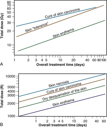
Figure 1-3 Isoeffect curves relating the log of the total dose to the log of the overall treatment time for various levels of skin reaction and the cure of skin cancer. A, Isoeffect curves were constructed by Cohen on the basis of a survey of earlier published data on radiotherapy equivalents.21–26 The slope of the curves for skin complications was 0.33, and the slope for tumor control was 0.22. B, The Strandqvist28 isoeffect curves were first published in 1944. All lines were drawn parallel and had a common slope of 0.33.
A, Adapted from Cohen L: Radiation response and recovery: Radiobiological principles and their relation to clinical practice. In Schwartz E, editor: The Biological Basis of Radiation Therapy, Philadelphia, 1966, JB Lippincott, p 208; B, adapted from Strandqvist M: Studien uber die kumulative Wirkung der Roentgenstrahlen bei Fraktionierung, Acta Radiol Suppl 55:1, 1944.
The first published isoeffect curves were produced by Strandqvist23 in 1944, and are also shown in Figure 1-3. When transformed on log-log coordinates, isoeffect curves for a variety of skin reactions, and the cure of skin cancer, were drawn as parallel lines, with common slopes of 0.33. These results implied that there would be no therapeutic advantage to using prolonged treatment times (i.e., multiple small fractions versus one or a few large doses) for the preferential eradication of tumors while simultaneously sparing normal tissues.24 It was somewhat ironic that the Strandqvist curves were so popular in the years that followed, when it was already known that the therapeutic ratio did increase (at least to a point) with prolonged, as opposed to very short, overall treatment times. However, the overarching advantage was that these isoeffect curves were quite reliable at predicting skin reactions, which were the dose-limiting factors at that time.
The “Golden Age” of Radiation Biology and Therapy: The Second 50 Years
Perhaps the defining event that ushered in the golden age of radiation biology was the publication of the first survival curve for mammalian cells exposed to graded doses of ionizing radiation.25 This first report of a quantitative measure of intrinsic radiosensitivity of a human cell line (HeLa, derived from a cervical carcinoma26) was published by Puck and Marcus25 in 1956. To put this seminal work in the proper perspective, however, it is first necessary to review the physicochemical basis for why ionizing radiation is toxic to biologic materials.
The Interaction of Ionizing Radiation with Biologic Materials
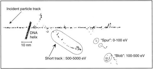
As mentioned in the introductory section of this chapter, ionizing radiation deposits energy as it traverses the absorbing medium through which it passes. The most important feature of the interaction of ionizing radiation with biologic materials is the random and discrete nature of the energy deposition. Energy is deposited in increasingly energetic packets referred to as “spurs” (100 eV or less deposited), “blobs” (100 to 500 eV), or “short tracks” (500 to 5000 eV), each of which can leave from approximately three to several dozen ionized atoms in its wake. This is illustrated in Figure 1-4, along with a segment of (interphase) chromatin shown to scale. The frequency distribution and density of the different types of energy deposition events along the track of the incident photon or particle are measures of the radiation’s linear energy transfer or LET (see also the “Relative Biologic Effectiveness” section, later). Because these energy deposition events are discrete, it follows that although the average amount of energy deposited in a macroscopic volume of biologic material may be rather modest, the distribution of this energy on a microscopic scale may be quite large. This explains why ionizing radiation is so efficient at producing biologic damage; the total amount of energy deposited in a 70-kg human that will result in a 50% probability of death is only about 70 calories, about as much energy as is absorbed by drinking one sip of hot coffee.27 The key difference is that the energy contained in the sip of coffee is uniformly distributed, not random and discrete.
Any and all cellular molecules are potential targets for the localized energy deposition events that occur in spurs, blobs, or short tracks. Whether the ionization of a particular biomolecule results in a measurable biologic effect depends on a number of factors, including how probable a target the molecule represents from the point of view of the ionizing particle, how important the molecule is to the continued health of the cell, how many copies of the molecule are normally present in the cell and to what extent the cell can react to the loss of “working copies,” and how important the cell is to the structure or function of its corresponding tissue or organ. DNA, for example, is obviously an important cellular macromolecule and one that is present only as a single double-stranded copy. On the other hand, other molecules in the cell may be less crucial to survival yet are much more abundant than DNA, and therefore have a much higher probability of being hit and ionized. The most abundant molecule in the cell by far is water, comprising some 80% to 90% of the cell on a per weight basis. The highly reactive free radicals formed by the radiolysis of water are capable of adding to the DNA damage resulting from direct energy absorption by migrating to the DNA and damaging it indirectly. This mechanism is referred to as “indirect radiation action” to distinguish it from the aforementioned “direct radiation action.”28 The direct and indirect action pathways for ionizing radiation are illustrated below.
The most highly reactive and damaging species produced by the radiolysis of water is the hydroxyl radical (•OH), although other free radical species are also produced in varying yields.29,30 Ultimately, it has been determined that cell killing by indirect action constitutes some 70% of the total damage produced in DNA for low LET radiation.
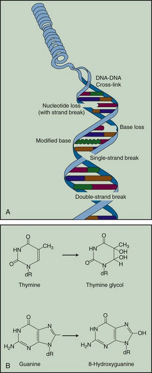
The •OH radical is capable of both abstraction of hydrogen atoms from other molecules and addition across carbon-carbon or other double bonds. More complex macromolecules that have been converted to free radicals can undergo a series of transmutations in an attempt to rid themselves of unpaired electrons, many of which result in the breakage of nearby chemical bonds. In the case of DNA, these broken bonds may result in the loss of a base or an entire nucleotide or in frank scission of the sugar phosphate backbone, involving one or both DNA strands. In some cases, chemical bonds are first broken but then rearranged, exchanged, or rejoined in inappropriate ways. Bases in DNA may be modified by the addition of one or more hydroxyl groups (e.g., the base thymine converted to thymine glycol), pyrimidines may become dimerized, and/or the DNA may become cross-linked to itself or to associated protein components. And again, because the initial energy deposition events are discrete, the free radicals produced also are clustered and therefore undergo their multiple chemical reactions and produce multiple damages in a highly localized area. This has been termed the “multiply-damaged site”31 or “cluster”32 hypothesis. Examples of the types of damage found in irradiated DNA are shown in Figure 1-5.
Biochemical Repair of DNA Damage
The study of DNA repair in mammalian cells received a significant boost during the late 1960s with publications by Cleaver33,34 that identified the molecular defect responsible for the human disease xeroderma pigmentosum (XP). Patients with XP are exquisitely sensitive to sunlight and highly cancer-prone (particularly to skin cancers). Cleaver showed that cells derived from such patients were likewise sensitive to UV radiation and defective in the nucleotide excision repair pathway (discussed later). These cells were not especially sensitive to ionizing radiation, however. Several years later, Taylor and colleagues35 reported that cells derived from patients with a second cancer-prone disorder called ataxia telangiectasia (AT) were extremely sensitive to ionizing radiation and radiation-mimetic drugs but not to UV radiation. In the years that followed, cell cultures derived from patients with these two conditions were used to help elucidate the complicated processes of DNA repair in mammalian cells.
Today, many rodent and human genes involved in DNA repair have been cloned.36 Nearly 20 distinct gene products participate in excision repair of base damage, and even more are involved in the repair of strand breaks. Many of these proteins function as component parts of larger repair complexes; some of these parts are interchangeable and participate in other DNA repair and replication pathways as well. It is also noteworthy that some are not involved with the repair process per se but rather link DNA repair to other cellular functions, including transcription, cell cycle arrest, chromatin remodeling, and apoptosis.37 This attests to the fact that the maintenance of genomic integrity results from a complex interplay between not only the repair proteins themselves but between others that serve as damage sensors, signaling mediators and transducers, and effectors.
For example, the defect responsible for the disease AT is not in a gene that codes for a repair protein but rather in a gene that participates in damage recognition and in a related pathway that normally prevents cells from entering S phase of the cell cycle and beginning DNA synthesis while residual DNA damage is present. This was termed the G1/S checkpoint response.38 Because of this genetic defect, AT cells do not experience the normal G1 arrest after irradiation and enter S phase with residual DNA damage. This accounts both for the exquisite radiosensitivity of AT cells and the resulting genomic instability that can lead to carcinogenesis.
What is known about the various types of DNA repair in mammalian cells is outlined below.
Base Excision Repair
The repair of base damage is initiated by DNA repair enzymes called DNA glycosylases, which recognize specific types of damaged bases and excise them without otherwise disturbing the DNA strand.39 The action of the glycosylase itself results in the formation of another type of damage observed in irradiated DNA—an apurinic or apyrimidinic (AP) site. The AP site is then recognized by another repair enzyme, an AP endonuclease, which nicks the DNA adjacent to the lesion. The resulting strand break becomes the substrate for an exonuclease, which removes the abasic site, along with a few additional bases. The small gap that results is patched by DNA polymerase, which uses the opposite, hopefully undamaged, DNA strand as a template. Finally, DNA ligase seals the patch in place.
Nucleotide Excision Repair
The DNA glycosylases that begin the process of base excision repair do not recognize all known forms of base damage, however, particularly bulky or complex lesions.39 In such cases, another group of enzymes, termed structure-specific endonucleases, initiate the excision repair process. These repair proteins do not recognize the specific lesion but are thought instead to recognize more generalized structural distortions in DNA that necessarily accompany a complex base lesion. The structure-specific endonucleases incise the affected DNA strand on both sides of the lesion, releasing an oligonucleotide fragment made up of the damage site and several bases on either side of it. Because a longer segment of excised DNA—including both bases and the sugar phosphate backbone—is generated, this type of excision repair is referred to as nucleotide excision repair to distinguish it from base excision repair (described earlier), where the initial step in the repair process is removal of the damaged base only. After this step, the remainder of the nucleotide excision repair process is similar to that of base excision repair; the gap is then filled in by DNA polymerase and sealed by DNA ligase. Overall, however, nucleotide excision repair is a much slower process, with a half-time of approximately 12 hours.
For both types of excision repair, active genes in the process of transcription are repaired preferentially and more quickly. This has been termed transcription-coupled repair.40
Strand Break Repair
Despite the fact that unrepaired or mis-rejoined strand breaks, particularly DSBs, often have the most catastrophic consequences for the cell in terms of loss of reproductive integrity,41 the way in which mammalian cells repair strand breaks has been more difficult to elucidate than the way in which they repair base damage. Much of what was originally discovered about these repair processes is derived from studies of x ray–sensitive rodent cells and microorganisms that were subsequently discovered to harbor specific defects in strand break repair. Since then, other human genetic diseases characterized by DNA repair defects have been identified and are also used to help probe these fundamental processes.
A genetic technique known as complementation analysis allows further characterization of genes involved in DNA repair. Complementation analysis involves the fusion of different strains of cells possessing the same phenotypic defect and subsequent testing of the hybrid cell for the presence or absence of this phenotype. Should two cell types bearing the defect yield a phenotypically normal hybrid cell, this implies that the defect has been “complemented” and that the defective phenotype must result from mutations in at least two different genes. With respect to DNA strand break repair, eight different genetic complementation groups have been identified in rodent cell mutants. For example, a mutant Chinese hamster cell line, designated EM9, seems especially radiosensitive owing to delayed repair of DNA single-strand breaks, a process that is normally complete within minutes of irradiation.42
With respect to the repair of DNA DSBs, the situation is more complicated in that the damage on each strand of DNA may be different, and, therefore, no intact template would be available to guide the repair process. Under these circumstances, cells depend on genetic recombination (nonhomologous end joining or homologous recombination43) to cope with the damage.
The BRCA1 and BRCA2 gene products are also implicated in HR (and, possibly, NHEJ as well) because they interact with the Rad51 protein. Defects in these genes are associated with hereditary breast and ovarian cancer.44
Mismatch Repair
The primary role of mismatch repair (MMR) is to eliminate from newly synthesized DNA errors such as base/base mismatches and insertion/deletion loops caused by DNA polymerase.45 Descriptively, this process consists of three steps: mismatch recognition and assembly of the repair complex, degradation of the error-containing strand, and repair synthesis. In humans, MMR involves at least five proteins, including hMSH2, hMSH3, hMSH6, hMLH1, and hPMS2, as well as other members of the DNA repair and replication machinery.
One manifestation of a defect in mismatch repair is microsatellite instability, mutations observed in DNA segments containing repeated sequence motifs.46 Collectively, this causes the cell to assume a hypermutable state (“mutator phenotype”) that has been associated with certain cancer predisposition syndromes, in particular, hereditary nonpolyposis colon cancer (HNPCC, sometimes called Lynch syndrome).47,48
Cytogenetic Effects of Ionizing Radiation
Most chromosome aberrations result from an interaction between two (or more; discussed later) damage sites, and, therefore, can be grouped into three different types of “exchange” categories. A fourth category is reserved for chromosome aberrations thought to result from a single damage site.49 These categories are described below, and representative types of aberrations from each category are shown in Figure 1-6:
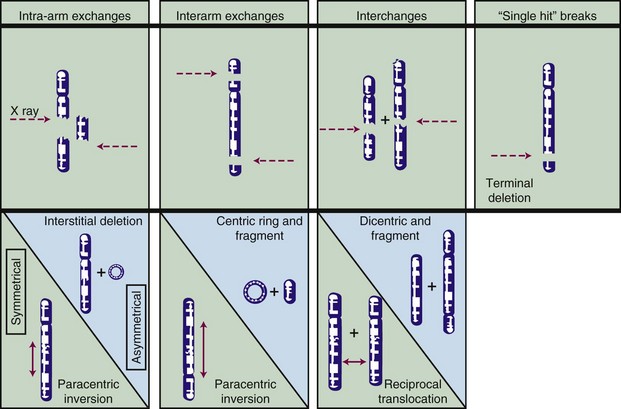
These four categories can be further subdivided according to whether the initial radiation damage occurred before or after the DNA is replicated during S phase of the cell cycle (a chromosome-type vs. a chromatid-type of aberration, respectively) and, for the three exchange categories, whether the lesion interaction was symmetric or asymmetric. Asymmetric exchanges always lead to the formation of acentric fragments that are usually lost in subsequent cell divisions and therefore are nearly always fatal to the cell. These fragments may be retained transiently in the cell’s progeny as extranuclear chromatin bodies called micronuclei. Symmetric exchanges are more insidious in that they do not lead to the formation of acentric fragments and the accompanying loss of genetic material at the next cell division, they are sometimes difficult to detect cytologically, and they are not invariably lethal to the cell. As such, they will be transmitted to all the progeny of the original cell. Some types of symmetric exchanges (a reciprocal translocation, for example) have been implicated in radiation carcinogenesis, insofar as they have the net effect of either bringing new combinations of genes together or of separating preexisting groups of genes.27 Depending on where in the genome the translocation takes place, genes normally on could be turned off, or vice versa, possibly with adverse consequences.


where α and β are proportionality constants related to the yields of the particular type of aberration and c is the spontaneous frequency of that aberration in unirradiated cells. For fractionated doses of low LET radiation, or continuous low-dose rates, the yield of exchange-type aberrations decreases relative to that for acute doses, and the dose-response curve tends to become more linear. For high LET radiations, dose-response curves for aberration induction become steeper (higher aberration yields) and more linear compared with those for low LET radiations.
Historically, exchange-type chromosome aberrations had been assumed to involve no more than two “breakpoints” that were presumably proximate in both space and time. However, by using fluorescent antibody probes or fluorescent in situ hybridization (FISH) to “paint” whole chromosomes, it is now clear that some exchanges are complex, that is, their formation requires at least three breakpoints in at least two chromosomes.50 Characterization of such complex chromosome aberrations should provide further insights into mechanisms of radiation-induced clustered damage in DNA, nuclear structure and organization, and DNA repair. Finally, another tantalizing finding is that high LET radiations tend to produce complex aberrations more readily than low LET radiations, suggesting that the presence of such could be a marker for exposure to high LET.51
Cell Survival Curves and Survival Curve Theory
What Is Meant by “Cell Death”?
The traditional definition of death as a permanent, irreversible cessation of vital functions is not the same as what constitutes death to the radiation biologist or oncologist. For proliferating cells—including those maintained in vitro, the stem cells of normal tissues, and tumor clonogens—cell death in the radiobiologic sense refers to a loss of reproductive integrity, that is, the cell has been rendered unable to sustain proliferation indefinitely. This type of “reproductive” or “clonogenic” death does not preclude the possibility that a cell may remain physically intact and metabolically active and able to continue its tissue-specific functions for some time after undergoing irradiation. In fact, some reproductively dead cells can even complete a few additional mitoses before finally succumbing to death in the more traditional sense.52
Apoptosis, or programmed cell death, is a type of nonreproductive or interphase death commonly associated with embryonic development and normal tissue remodeling and homeostasis.53 However, certain normal tissue and tumor cells also undergo apoptosis following irradiation, including normal cells of hematopoietic or lymphoid origin or crypt cells of the small intestine and salivary gland, plus some experimental tumor cell lines of gynecologic and hematologic origin.54 Cells undergoing apoptosis exhibit a number of characteristic morphologic (e.g., nuclear condensation and fragmentation, membrane blebbing) and biochemical (DNA degradation) changes that culminate in the fragmentation and lysis of the cell, often within 12 hours of irradiation and before the first postirradiation mitosis. Ultimately, the remains of apoptotic cells are phagocytized by neighboring cells and therefore do not cause the type of inflammatory response, tissue destruction, and disorganization characteristic of necrosis. Apoptosis is an active and carefully regulated pathway that involves several genes and gene products and an appropriate stimulus that activates the pathway. The molecular biology of apoptosis, the apoptosis-resistant phenotype noted for many types of tumor cells, and the role that radiation may play in the process are discussed in detail in Chapter 2.
Most assays of radiosensitivity of cells and tissues, including those described below, use reproductive integrity, either directly or indirectly, as an endpoint. Although such assays have served the radiation oncology community well in terms of elucidating dose-response relationships for normal tissues and tumors, it is now clear that reproductive death is not necessarily the whole story. What remains unclear is whether and to what extent apoptosis contributes to our traditional measures of radiosensitivity based on reproductive integrity, and whether pretreatment assessment of apoptotic propensity in tumors or dose-limiting normal tissues is of prognostic significance. The interrelationships between these different pathways of cell death can be quite complex. Meyn,54 for example, has suggested that a tumor with a high spontaneous apoptotic index may be inherently more radiosensitive because cell death might be triggered by lower doses than are usually required to cause reproductive death. Also, tumors that readily undergo apoptosis may have higher rates of cell loss, the net effect of which would be to partially offset cell production, thereby reducing the number of tumor clonogens. On the other hand, not all types of tumor cells undergo apoptosis, and even among those that do, radiotherapy itself could have the undesirable side effect of selecting for subpopulations of cells that are already apoptosis-resistant.
Cell Survival and Dose-Response Curve Models
As had been the case during the early years of radiation therapy, advances in radiation physics, specifically biophysics, preceded advances in radiation biology. Survival curve theory originated in a consideration of the physics of energy deposition in matter by ionizing radiation. Early experiments with macromolecules and prokaryotes established the fact that dose-response relationships could be explained, in principle, by the random and discrete nature of energy absorption, if it was assumed that the response resulted from critical “targets” receiving random “hits.”55 With an increasing number of shouldered survival and dose-response curves being described for cells irradiated both in vitro and in vivo, various equations were developed to fit these data. Target theory pioneers studied a number of different endpoints in the context of target theory, including enzyme inactivation in cell-free systems,28 cellular lethality, chromosomal damage, and radiation-induced cell cycle perturbations in microorganisms.28,56 Survival curves, in which the log of the “survival” of a certain biologic activity was plotted as a function of the radiation dose, were found to be either exponential or sigmoid in shape, the latter usually noted for the survival of more complex organisms.28
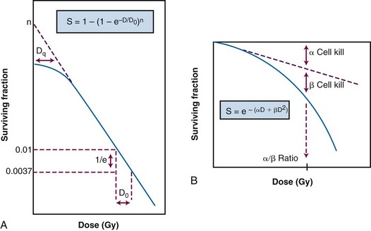
 . In this equation, S is the fraction of cells that survive a given dose, D, and D0 is the dose increment that reduces the cell survival to 37% (1/e) of some initial value on the exponential portion of the curve (i.e., a measure of the reciprocal of the slope). The sigmoid survival curves, characterized by a shoulder at low doses, were consistent with target theory if one assumed that either multiple targets or multiple hits in a single target (or a combination of both) were necessary for radiation inactivation. A mathematical expression based on target theory that provided a fairly good fit to survival data was S = 1 − (1 −
  )n, with n being the back extrapolation of the exponential portion of the survival curve to zero dose (i.e., a measure of the width of the shoulder). Implicit in this multitarget model was that damage had to accumulate before the overall effect was registered.
It soon became apparent that some features of this model were inadequate.57 The most obvious problem was that the single-hit, multitarget equation predicted that survival curves should have initial slopes of zero, that is, that for vanishingly small doses (e.g., repeated small doses per fraction or continuous low dose-rate exposure), the probability of cell killing would approach zero. This was decidedly not what was observed in practice for either mammalian cell survival curves or as inferred from clinical studies in which highly fractionated or low dose-rate treatment schedules were compared with more conventional fractionation. There was no fractionation schedule that produced essentially no cell killing, all other radiobiologic factors being equal.
A somewhat different interpretation of cell survival was proposed by Kellerer and Rossi58 during the late 1960s and early 1970s. The linear-quadratic or “alpha-beta” equation, S =  , was shown to fit many survival data quite well, particularly in the low-dose region of the curve, and also provided for the negative initial slope investigators had described.57 In this expression, S is again the fractional cell survival following a dose D, α is the rate of cell kill by a single-hit process, and β is the rate of cell kill by a two-hit mechanism.
The theoretical derivation of the linear-quadratic equation is based on two very different sorts of observations. Based on microdosimetric considerations, Kellerer and Rossi57 proposed that a radiation-induced lethal lesion resulted from the interaction of two sublesions. According to this interpretation, the αD term is the probability of these two sublesions being produced by a single event (the “intra-track” component), whereas βD2 is the probability of the two sublesions being produced by two separate events (the “inter-track” component). Chadwick and Leenhouts59 derived the same equation based on a different set of assumptions, namely that a DSB in DNA was a lethal lesion and that such a lesion could be produced by either a single energy deposition involving both strands of DNA or by two separate events, each involving a single strand.
A comparison of the features and parameters of the target theory and linear-quadratic survival curve expressions is shown in Figure 1-7.
Clonogenic Assays In Vitro
As mentioned previously, it was not until the mid-1950s that mammalian cell culture techniques were sufficiently refined to allow quantitation of the radiation responses of single cells.60,61 The Puck and Marcus25 acute-dose, x-ray survival curve for the human tumor cell line HeLa is shown in Figure 1-8. Following graded x-ray doses, the reproductive integrity of single HeLa cells was measured by their ability to form macroscopic colonies of at least 50 cells (corresponding to approximately six successful postirradiation cell divisions) on Petri dishes.
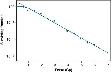
A number of features of this survival curve were of particular interest. First, qualitatively at least, the curve was similar in shape to those previously determined for many microorganisms, being characterized by a shoulder at low doses and a roughly exponential region at high doses. Of note, however, was the finding that the D0 for HeLa cells was only 96 R, some 10-fold to 100-fold less than any D0 determined for microorganisms, and 1000-fold to 10,000-fold less than any D0 for the inactivation of isolated macromolecules.52 Thus cellular reproductive integrity was found to be a much more radiosensitive endpoint for HeLa cells than for prokaryotes or primitive eukaryotes. The value of the extrapolation number, n, for HeLa cells was approximately 2.0, indicating that the survival curve did have a small shoulder, but again, much smaller than that typically observed for microorganisms. Puck and Marcus25 suggested that the n value was a reflection of the number of critical targets in the cell, each requiring a single hit before the cell would be killed, and further postulated that the targets were, in fact, the chromosomes themselves. However, the potential pitfalls of deducing mechanisms of radiation action from parameters of a descriptive survival curve model were soon realized.62,63
Clonogenic Assays In Vivo
To bridge the gap between the radiation responses of cells grown in culture and in an animal, Hewitt and Wilson64 developed an ingenious method to assay single cell survival in vivo. Lymphocytic leukemia cells obtained from the livers of donor CBA mice were harvested, diluted, and inoculated into disease-free recipient mice. By injecting different numbers of donor cells, a standard curve was constructed that allowed a determination of the average number of injected cells necessary to cause leukemia in 50% of the recipient mice. It was determined that the endpoint of this titration, the “50% take dose” or TD50, corresponded to an inoculum of a mere two leukemia cells. Using this value as a reference, Hewitt and Wilson then injected leukemia cells harvested from gamma-irradiated donor mice into recipients and again determined the TD50 following different radiation exposures. In this way, the surviving fraction after a given radiation dose could be calculated from the ratio of the TD50 for unirradiated cells to that for irradiated cells. Using this technique, a complete survival curve was constructed that had a D0 of 162 R and an n value close to 2.0, values quite similar to those generated for cell lines irradiated in vitro. For the most part, in vivo survival curves for a variety of cell types were also similar to corresponding in vitro curves.
A similar trend was apparent when in vivo survival curves for nontumorigenic cells were first produced. The first experiments by Till and McCulloch65,66 using normal bone marrow stem cells were inspired by the knowledge that failure of the hematopoietic system was a major cause of death following total body irradiation and that lethally irradiated animals could be “rescued” by a bone marrow transplant. The transplanted viable bone marrow cells were observed to form discrete nodules or colonies in the otherwise sterilized spleens of irradiated animals.
Subsequently, these authors transplanted known quantities of irradiated donor bone marrow into lethally irradiated recipient mice and were able to count the resulting splenic nodules and then calculate the surviving fraction of the injected cells in much the same way as was done for in vitro experiments. The D0 for mouse bone marrow was 0.95 Gy.66 Other in vivo assay systems based on the counting of colonies or nodules included the skin epithelium assay of Withers,67 the intestinal crypt assays of Withers and Elkind,68,69 and the lung colony assay of Hill and Bush.70 During the late 1960s and early 1970s, it also became possible to do excision assays, in which tumors irradiated in vivo were removed and enzymatically dissociated and single cells from the tumors were plated for clonogenic survival in vitro, thereby allowing more quantitative measurement of survival and avoiding some of the pitfalls of in vivo assays.71
Non-Clonogenic Assays In Vivo
Another widely used nonclonogenic method to assess normal tissue radioresponse is the skin reaction assay, originally developed by Fowler and colleagues.72 Pigs were often used because their skin is similar to that of humans in several key respects. An ordinate scoring system was used to compare and contrast different radiation schedules and was derived from the average severity of the skin reaction noted during a certain time period (specific to the species and whether the endpoint occurred early or late) following irradiation. For example, for early skin reactions, a skin score of “1” might correspond to mild erythema, whereas a score of “4” might correspond to confluent moist desquamation over more than half of the irradiated area.
Finally, two common nonclonogenic assays for tumor response are the growth delay/regrowth delay assay73 and the tumor control dose assay.74 Both assays are simple and direct, are applicable to most solid tumors, and are clinically relevant. The growth delay assay involves the periodic measurement of a tumor’s dimensions as a function of time after irradiation and a calculation of the tumor’s approximate volume. For tumors that regress rapidly during and after radiotherapy, the endpoint scored is typically the time in days it takes for the tumor to regrow to its original volume at the start of irradiation. For tumors that regress more slowly, a more appropriate endpoint might be the time it takes for the tumor to grow or regrow to a specified size, such as three times its original volume. Dose-response curves are generated by plotting the amount of growth delay as a function of radiation dose.
Cellular “Repair”: Sublethal and Potentially Lethal Damage Recovery
Taking the cue from target theory that the shoulder region of the radiation survival curve indicated that “hits” had to accumulate prior to cell killing, Elkind and Sutton75,76 sought to better characterize the nature of the damage caused by these hits and how the cell processed this damage. Even in the absence of any detailed information about DNA damage and repair at that time, a few things seemed obvious. First, those hits or damages that were registered as part of the accumulation process yet did not in and of themselves produce cell killing were, by definition, sublethal. Second, sublethal damage only became lethal when it interacted with additional sublethal damage, that is, when the total amount of damage had accumulated to a sufficient level to cause cell lethality. But what would be the result of deliberately interfering with the damage accumulation process by, for example, delivering part of the intended radiation dose, inserting a radiation-free interval, and then delivering the remainder of the dose? The results of such “split-dose” experiments were crucial to the understanding of why and how fractionated radiation therapy works as it does. The discovery and characterization of sublethal damage, as low-tech and operational as the concept may be by today’s standards, still stands as arguably the single most important contribution radiation biology has made to the practice of radiation oncology.
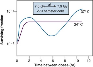
Of additional interest was the observation that the shape of the split-dose recovery curve varied with the temperature during the radiation-free interval (Figure 1-9). When the cells were maintained at room temperature between the split doses, the SLDR curve rose to a maximum after about 2 hours and then leveled off. When the cells were returned to a 37° C incubator for the radiation-free interval, a different pattern emerged. Initially, the split-dose recovery curve rose to a maximum after 2 hours, but then the curve exhibited a series of oscillations, dropping to a second minimum at about 4 to 5 hours, and then rising again to a higher maximum for split-dose intervals of 10 hours or more. The interpretation of this pattern of SLDR was that other radiobiologic phenomena operated simultaneously with cellular recovery. In this case, the fine structure of the split-dose recovery curve was not caused by an oscillating repair process but rather by a superimposed cell cycle effect: the so-called radiation “age response” through the cell cycle. This is discussed in detail in the “Ionizing Radiation and the Cell Cycle” on the facing page (see also Figure 1-14).
Since Elkind and Sutton’s original work, SLDR kinetics have been described for many different types of mammalian cells in culture52 and for most normal and tumor tissues in vivo.77,78 Pertinent findings include:
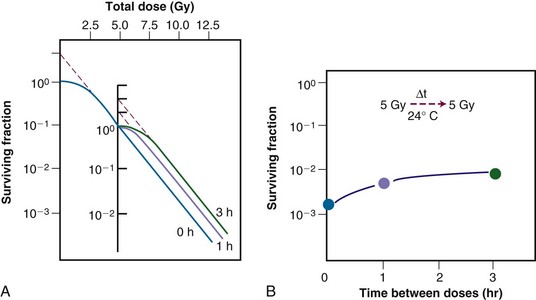
Figure 1-10 Sublethal damage recovery manifests as a return of the shoulder on the radiation survival curve when a total dose is delivered as two fractions separated by a time interval (A). If the interfraction interval is shorter than the time it takes for this recovery to occur, the shoulder will only be partially regenerated (compare the shoulder regions of the survival curves for intervals of 1 vs. 3 hours). Regeneration of the shoulder (B) accounts for the observed survival increase in the corresponding split-dose assay (see Fig. 1-9).
A second type of cellular recovery following irradiation is termed potentially lethal damage repair or recovery (PLDR) and was first described for mammalian cells by Phillips and Tolmach79 in 1966. PLD is, by definition, a spectrum of radiation damage that may or may not result in cell lethality depending on the cells’ postirradiation conditions. Conditions that favor PLDR include maintenance of cells in overcrowded conditions (plateau phase or contact-inhibited80,81 phase) and incubation following irradiation at reduced temperature,82 in the presence of certain metabolic inhibitors,79 or in balanced salt solutions rather than complete culture medium.82 What these treatment conditions have in common is that they are suboptimal for continued growth of cells. Presumably, resting cells (regardless of why they are resting) have more opportunity to repair DNA damage prior to cell division than cells that continue traversing the cell cycle immediately after irradiation. Phillips and Tolmach79 were the first to propose this repair-fixation or “competition” model to explain PLDR.
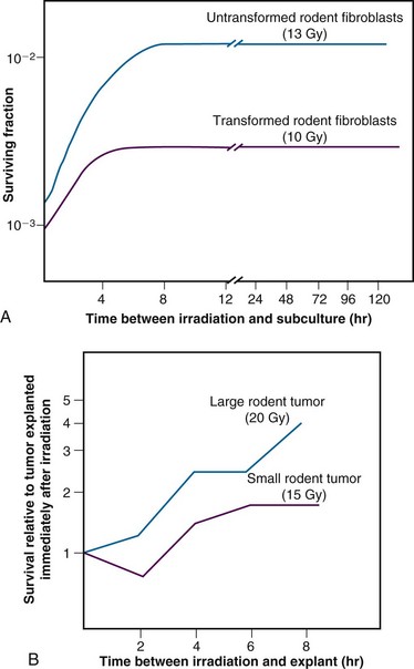
Admittedly, some of these postirradiation conditions are not likely to be encountered in vivo, but slow growth of cells in general, with or without a large fraction of resting cells, is a common characteristic of intact tissues. As might be expected, tumors (and, subsequently, select normal tissues amenable to clonogenic assay) were shown to repair PLD.81 Experiments using rodent tumors were modeled after comparable studies using plateau phase cells in culture, that is, a “delayed plating” assay was used. For such an experiment, the protocol involves irradiating the cell culture or animal tumor and then leaving the cells of interest in a confluent state (either in the overcrowded cell culture or in the intact tumor in the animal) for varying lengths of time before removing them, dissociating them into single cell suspensions, and plating the cells for clonogenic survival at a low density. The longer the delay between irradiation and the clonogenic assay, the higher the resulting surviving fraction of individual cells, even though the radiation dose is the same. In general, survival rises to a maximum within 4 to 6 hours and levels off thereafter (Figure 1-12).
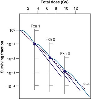
The kinetics and extent of recovery from both SLD and PLD have been correlated with the molecular repair of DNA and the rejoining of chromosome breaks.83,84 For the purposes of radiation therapy, however, the most important consideration is that both processes have the potential to increase the surviving fraction of cells between subsequent dose fractions. Such a survival increase would be manifest clinically as either increased normal tissue tolerance or decreased tumor control. It is also important to appreciate that small differences in recovery capacity between normal and tumor cells after one dose fraction are magnified into large differences after 30 or more dose fractions.
Ionizing Radiation and the Cell Cycle
Advances in techniques for the study of cell cycle kinetics during the 1950s and 1960s paved the way for the analysis of radiation responses of cells as a function of “age.” Using a technique known as autoradiography that involved the incubation of cells with radioactive DNA precursors, followed by the detection of cells that had incorporated such precursors by their ability to expose radiographic film, Howard and Pelc85 were able to identify the S, or DNA synthesis, phase of the cell cycle. When combined with the other cytologically obvious cell cycle marker, mitosis, they were able to discern the four phases of the cell cycle for actively growing cells: G1, S, G2, and M.
Methodology
Several techniques were subsequently developed for the collection of synchronized cells in vitro. One of the most widely used was the mitotic harvest or “shake-off” technique first described by Terasima and Tolmach.86,87 By shaking cultures, mitotic cells, which tend to round up and become loosely attached to the culture vessel’s surface, can be dislodged, collected along with the overlying growth medium, and inoculated into new culture flasks. By incubating these flasks at 37° C, cells begin to proceed synchronously into G1 phase (and semisynchronously thereafter). Thus, by knowing the length of the various phase durations for the cell type being studied and then delivering a radiation dose at a time of interest after the initial synchronization, the survival response of cells in different phases of the cell cycle can be determined.
A second synchronization method involved the use of DNA synthesis inhibitors such as fluorodeoxyuridine88 and, later, hydroxyurea89 to selectively kill S phase cells yet allow cells in other phases to continue cell cycle progression until they become blocked at the border of G1 and S phase. By incubating cells in the presence of these inhibitors for times sufficient to collect nearly all cells at the block point, large numbers of cells can be synchronized. In addition, the inhibitor technique has two other advantages, namely that some degree of synchronization is possible in vivo90 as well as in vitro and that by inducing synchrony at the end of G1 phase, a higher degree of synchrony can be maintained for longer periods than if synchronization had been at the beginning of G1. On the other hand, the mitotic selection method does not rely on the use of agents that could perturb the normal cell cycle kinetics of the population under study.
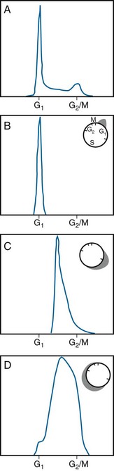
Developments in the early 1970s provided what are now considered some of the most valuable tools for the study of cytokinetic effects: the flow cytometer and its offshoot, the fluorescence-activated cell sorter.91 These have largely replaced the aforementioned longer and more labor intensive cell cycle synchronization methods. Using this powerful technique, single cells are stained with a fluorescent probe that binds stoichiometrically to a specific cellular component, DNA in the case of cell cycle distribution analysis. The stained cells are then introduced into a pressurized flow cell and forced to flow single file and at a high rate of speed through an intense, focused laser beam that excites the fluorescent dye. The resulting light emission from each cell is collected by photomultiplier tubes and recorded. Then a frequency histogram of cell number as a function of relative fluorescence, is generated, with the amount of light output being directly proportional to DNA content of each cell examined. Accordingly, cells with a “1X” DNA content would correspond to cells in G1 phase, cells with a “2X” DNA content, in G2 or M phase, and cells with DNA contents between “1X” and “2X,” in the S phase of the cell cycle. By performing a mathematical fit to the DNA histogram, the proportion of cells in each phase of the cell cycle can be determined, the phase durations can be derived, and differences in DNA ploidy can be identified. DNA flow cytometry is quite powerful in that not only can a static measure of cell cycle distribution be obtained for a cell population of interest but, also, dynamic studies of, for example, transit through the various cell cycle phases, or treatment-induced kinetic perturbations, can be monitored over time (Figure 1-13). A flow cytometer can be outfitted to include a cell-sorting feature; in this case, cells analyzed for a property of interest can be collected in separate “bins” after they pass through the laser beam and, if possible, used for other experiments.
Age Response Through the Cell Cycle
Results of an age response experiment of Terasima and Tolmach,87 using synchronized HeLa cells, are shown in the lower panel of Figure 1-14. Following a single dose of 5 Gy of x rays, cells were noted to be most radioresistant in late S phase. Cells in G1 were resistant at the beginning of the phase but became sensitive toward the end of the phase, and G2 cells were increasingly sensitive as they moved toward the highly sensitive M phase. In subsequent experiments by Sinclair,92,93 age response curves for synchronized Chinese hamster V79 cells showed that the peak in resistance observed in G1 HeLa cells was largely absent for V79 cells. This is also illustrated in Figure 1-14 (upper panel). Otherwise, the shapes of the age response curves for the two cell lines are similar. The overall length of the G1 phase determines whether the resistant peak in early G1 will be present; in general, this peak of relative radioresistance is only observed for cells with long G1 phases. For cells with short G1 phases, the entire phase is often intermediate in radiosensitivity. An analysis of the complete survival curves for synchronized cells93,94 confirms that the most sensitive cells are those in M and late G2 phase, in which survival curves are steep and largely shoulderless, and the most resistant cells are those in late S phase. The resistance of these cells is conferred by the presence of a broad survival curve shoulder rather than by a significant change in survival curve slope (Figure 1-15). When high LET radiations are used, the age response variation through the cell cycle is significantly reduced or eliminated, since survival curve shoulders are either decreased or removed altogether by such exposures (see also “Relative Biologic Effectiveness,” discussed later). Similar age response patterns have been identified for cells synchronized in vivo.90
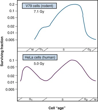
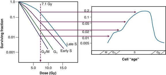
Figure 1-15 Cell survival curves for irradiated populations of Chinese hamster cells synchronized in different phases of the cell cycle (left panel), illustrating how these radiosensitivity differences translate into the age-response patterns shown in the right panel (see Fig. 1-14).
The existence of a cell cycle age response for ionizing radiation provided an explanation for the unusual pattern of SLDR observed for cells maintained at 37° C during the recovery interval (see Figure 1-9). In Elkind and Sutton’s experiments, exponentially-growing cells were used, that is, cells that were asynchronously distributed across the different phases of the cell cycle. The cells that survived irradiation tended to be those most radioresistant. As such, the remaining population was enriched with the more resistant cells and partially synchronized. For low LET radiation, those cells that were most resistant were the cells that were in S phase at the time of the first radiation dose. However, at 37° C, cells continued to progress through the cell cycle, so those surviving cells in S phase at the time of the first dose may have moved into G2 phase by the time the second dose was delivered. Thus the observed survival nadir in the SLDR curve was not due to a loss or reversal of repair but rather, because the population of cells was now enriched in G2 phase cells, which are inherently more radiosensitive. For even longer radiation-free intervals, it is possible that the cells surviving the first dose would transit from G2 to M, and back into G1 phase, dividing and doubling their numbers. In this case, the SLDR curve again shows a surviving fraction increase because the number of cells has increased. None of these cell cycle–related phenomena occur when the cells are maintained at room temperature during the radiation-free interval because movement through the cell cycle is inhibited under such conditions; in that case, all that is noted is the initial survival increase due to prompt SLDR.
Radiation-Induced Cell Cycle Blocks and Delays
Radiation is capable of disrupting the normal proliferation kinetics of cell populations. This was recognized by Canti and Spear95 in 1927 and studied in conjunction with radiation’s ability to induce cellular lethality. With the advent of mammalian cell culture and synchronization techniques and time-lapse cinemicrography, it became possible for investigators to study mitotic and division delay phenomena in greater detail.
Mitotic delay, defined as a delay in the entry of cells into mitosis, is a consequence of “upstream” blocks or delays in the movement of cells from one cell cycle phase to the next. Division delay, a delay in the time of appearance of new cells at the completion of mitosis, is caused by the combined effects of mitotic delay and any further lengthening of the mitosis process itself. Division delay increases with dose, and is, on average, about 1 to 2 hours per Gray,87 depending on the cell line.
The cell cycle blocks and delays primarily responsible for mitotic and division delay are, respectively, a block in the G2-to-M phase transition and a block in the G1-to-S phase transition. The duration of the G2 delay, like the overall division delay, varies with cell type, but for a given cell type is both dose and cell cycle age dependent. In general, the length of the G2 delay increases linearly with dose. For a given dose, the G2 delay is longest for cells irradiated in S or early G2 phase and shortest for cells irradiated in G1 phase.101 Another factor contributing to mitotic and division delay is a block in the flow of cells from G1 into S phase. For x-ray doses of about 6 Gy and above, there is a 50% decrease in the rate of tritiated thymidine uptake in exponentially growing cultures of mouse L cells. Little96 reached a similar conclusion from G1 delay studies using human liver LICH cells maintained as confluent cultures.
A possible role for DNA damage and its repair in the etiology of division delay was bolstered by the finding that certain cell types that either did not exhibit the normal cell cycle delays associated with radiation exposure (such as AT cells)38 or, conversely, were treated with chemicals (such as caffeine) that ameliorated the radiation-induced delays97 tended to contain higher amounts of residual DNA damage and to show increased radiosensitivity.
It is now known that the radiation-induced perturbations in cell cycle transit are under the control of cell cycle checkpoint genes, whose products normally govern the orderly (and unidirectional) flow of cells from one phase to the next. The checkpoint genes are responsive to feedback from the cell as to its general condition and readiness to transit to the next cell cycle phase. DNA integrity is one of the criteria used by these genes to help make the decision whether to continue traversing the cell cycle or to pause, either temporarily or, in some cases, permanently. Cell cycle checkpoint genes are discussed in Chapter 2.
Redistribution in Tissues
Because of the age response through the cell cycle, an initially asynchronous population of cells surviving a dose of radiation becomes enriched with S phase cells. Because of variations in the rate of further cell cycle progression, however, this partial synchrony decays rapidly. Such cells are said to have “redistributed”98 with the net effect of sensitizing the population as a whole to a subsequent dose fraction (relative to what would have been expected had the cells remained in their resistant phases). A second type of redistribution, in which cells accumulate in G2 phase (in the absence of cell division) during the course of multifraction or continuous irradiation because of a buildup of radiation-induced cell cycle blocks and delays, also has a net sensitizing effect. This has been observed during continuous irradiation by several investigators,99 and in some of these cases, a net increase in radiosensitivity is seen at certain dose rates. This so-called “inverse dose rate effect,” where certain dose rates are more effective at cell killing than other, higher dose rates, was extensively studied by Bedford and associates.100 The magnitude of the sensitizing effect of redistribution varies with cell type depending on which dose rate is required to stop cell division. For dose rates below the critical range that causes redistribution, some cells can escape the G2 block and proceed on to cell division.
Densely Ionizing Radiation
Linear Energy Transfer (LET)
LET is a function both of the charge and the mass of the ionizing particle. For example, photons set in motion fast electrons that have a net negative charge but a negligible mass. Neutrons on the other hand give rise to recoil protons or α-particles that possess one or two positive charges, respectively, and are orders of magnitude more massive than electrons. Neutrons therefore have a higher LET than photons and are said to be densely ionizing, whereas x or gamma rays are considered sparsely ionizing. The LET concept is illustrated in Figure 1-16 for both densely and sparsely ionizing radiations. For a given ionizing particle, the rate of energy deposition in the absorbing medium also increases as the particle slows down. Therefore, a beam of radiation can only be described as having an average value for LET.
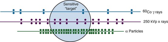
Representative LET values for types of radiations that have been used for radiation therapy include 0.2 keV/µm for cobalt-60 (60Co) gamma rays; 2.0 keV/µm for 250 kVp x rays; approximately 0.5 to 5.0 keV/µm for protons of different energies; approximately 50 to 150 keV/µm for neutrons of varying energy; 100 to 150 keV/µm for alpha particles; and 100 to 2500 keV/µm for “heavy ions.” (In general, for a given type of radiation, the LET decreases with increasing energy.)
Relative Biologic Effectiveness
Because high LET radiations are more densely ionizing than their low LET counterparts, it follows that energy deposition in a particular “micro” target volume will be greater, and, therefore, more severe damage to biomolecules would be anticipated. In this case, the fraction of cell killing attributable to irreparable and unmodifiable DNA damage increases in relation to that caused by the accumulation of sublethal damage. As such, a number of radiobiologic phenomena commonly associated with low LET radiation are decreased or eliminated with high LET radiation. For example, there is little, if any, sublethal52 or potentially lethal damage recovery.101 This is manifest as a reduction or loss of the shoulder of the acute-dose radiation survival curve, little or no sparing effect of dose fractionation or dose rate, and a corresponding reduction in the tolerance doses for normal tissue complications, particularly for late effects.102 Variations in the age response through the cell cycle are reduced or eliminated for high LET radiation,90 and the oxygen enhancement ratio (OER), a measure of the differential radiosensitivity of poorly oxygenated versus well-oxygenated cells (discussed later), decreases with increasing LET.103 The dependence of OER on LET is illustrated in Figure 1-17; at an LET of approximately 100 keV/µm, the relative radioresistance of hypoxic cells is eliminated.
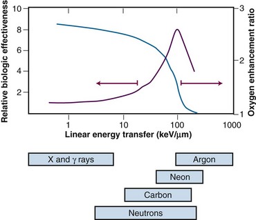
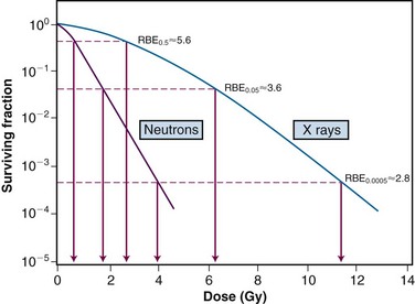
In light of these differences between high and low LET radiations, the term relative biologic effectiveness (RBE) has been used to compare and contrast two radiation beams of different LETs. RBE is defined as the ratio of doses of a known type of low LET radiation (historically, 250 kVp x rays were the standard, but 60Co gamma rays also can be used) to that of a higher LET radiation, to yield the same biologic endpoint. However, RBE does not increase indefinitely with increasing LET but reaches a maximum at approximately 100 keV/µm and then decreases again, yielding approximately a bell-shaped curve.
Factors that Influence Relative Biologic Effectiveness
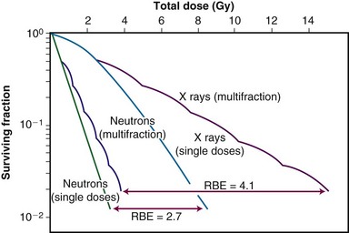
Relative biologic effectiveness is highly variable and depends on several irradiation parameters, including the type of radiation, total dose, dose rate, dose fractionation pattern, and biologic effect being assayed. As such, when quoting an RBE value, the exact experimental conditions used to measure it must be stated. Because increasing LET differentially reduces the shoulder region of the radiation survival curve compared with its exponential or near-exponential high-dose region, the single-dose RBE increases with decreasing dose (Fig. 1-18). Second, the RBE determined by comparing two isoeffective acute doses is less than the RBE calculated from two isoeffective (total) doses given either as multiple fractions or at a low dose rate. This occurs because the sparing effect of fractionation magnifies differences in the initial slope or shoulder region of cell survival or tissue dose response curves (Fig. 1-19).
The Oxygen Effect
Perhaps the best-known chemical modifier of radiation action is molecular oxygen. As early as 1909, Schwarz recognized that applying pressure to skin and thereby decreasing blood flow (and oxygen supply) caused a reduction in radiation-induced skin reactions.104 For many decades thereafter, radiation oncologists and biologists continued to suspect that the presence or absence of oxygen was capable of modifying radiosensitivity. In 1955, however, Thomlinson and Gray105 brought this concept to the forefront of radiobiology and formed the basis of the third major approach to the problem of the differential response of cells to radiotherapy, namely, that a change in the proportion of hypoxic cells in a tissue could alter its radioresponsiveness. Although commonly considered a problem for radiation therapy, hypoxia nevertheless has one particularly attractive feature: built-in specificity for tumors, to the extent that most normal tissues contain few, if any, hypoxic cells.
By studying histologic sections of a human bronchial carcinoma, Thomlinson and Gray105 noted that necrosis was always seen in the centers of cylindrical tumor cords having a radius in excess of 200 µm. Further, regardless of how large the central necrotic region was, the sheath of apparently viable cells around the periphery of this central region never had a radius greater than about 180 µm. The authors went on to calculate the expected maximum diffusion distance of oxygen from blood vessels located in the normal tissue stroma and found that the value of 150 to 200 µm agreed quite well with the radius of the sheath of viable tumor cells observed histologically. (With the advent of more sophisticated and quantitative methods for measuring oxygen utilization in tissues, the average diffusion distance of oxygen has since been revised downward to approximately 70 µm.27) Thus the oxygenation status of tumor cells varied from fully oxic to completely anoxic depending on where the cells were located in relation to the nearest blood vessels. It was inferred from these studies that cells at intermediate distances from the blood supply would be hypoxic and radioresistant yet remain clonogenic.
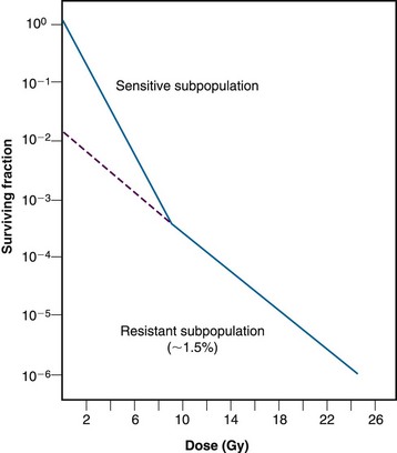
The first unambiguous demonstration that a solid animal tumor contained viable, radioresistant hypoxic cells was that of Powers and Tolmach106 in 1963; they used the dilution assay to generate an in vivo survival curve for mouse lymphosarcoma cells. The survival curve for this solid tumor was biphasic, having an initial D0 of about 1.1 Gy and a final D0 of 2.6 Gy (Fig. 1-20). Because the survival curve for lymphoid cells is shoulderless, it was rather simple to back-extrapolate the shallower component of the curve to the surviving fraction axis and determine that the resistant fraction of cells constituted about 1.5% of the total population. This was considered compelling evidence (yet did not prove) that this subpopulation of cells was both hypoxic and clonogenic.
The question then became how to prove that this small fraction of tumor cells was radioresistant because of hypoxia, as opposed to being radioresistant for other reasons. An elegant if somewhat macabre method was developed to address this dilemma, called the “paired survival curve technique.”106,107 In this assay, laboratory animals bearing tumors were divided into three treatment groups; one group was irradiated while breathing air, a second group irradiated while breathing 100% oxygen, and a third group killed by cervical dislocation and then promptly irradiated. Within each group, animals received graded radiation doses so that complete survival curves were generated for each treatment condition. When completed, the paired survival curve method yielded three different tumor cell survival curves: a fully oxic curve (most radiosensitive), a fully hypoxic curve (most radioresistant), and a survival curve for air-breathing animals, which, if the tumor contained viable hypoxic cells, was biphasic and positioned between the other two curves. It was then possible to mathematically strip the fully aerobic and hypoxic curves from the curve for air-breathing animals and determine the radiobiologically hypoxic fraction.
Across a variety of rodent tumors, the percentage of hypoxic cells was found to vary between nil and 50%, with an average of about 15%.107
Mechanistic Aspects of the Oxygen Effect
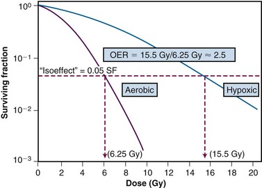
A more rigorous analysis of the nature of the oxygen effect is possible with cells or bacteria grown in vitro. Historically, oxygen had been termed a “dose-modifying agent,” that is, that the ratio of doses to achieve a given survival level under hypoxic and aerated conditions was constant, regardless of the survival level chosen. This dose ratio to produce the same biologic endpoint is termed the oxygen enhancement ratio, or OER, and is used for comparative purposes (Fig. 1-21). The OER typically has a value of between 2.5 and 3.0 for large single doses of x or gamma rays, 1.5 to 2.0 for radiations of intermediate LET, and 1.0 (i.e., no oxygen effect) for high LET radiations.
Increasingly, there is evidence that oxygen is not strictly dose-modifying. Several studies have shown that the OER for sparsely ionizing radiation is lower at lower doses than at higher doses. Lower OERs for doses per fraction in the range commonly used in radiotherapy have been inferred indirectly from clinical and experimental tumor data and more directly in experiments with cells in culture.108,109 It has been suggested that the lower OERs result from an age response for the oxygen effect, not unlike the age responses for radiosensitivity and cell cycle delay.27 Assuming cells in G1 phase of the cell cycle have a lower OER than those in S phase, and because G1 cells are also more radiosensitive, they would tend to dominate the low-dose region of the cell survival curve.
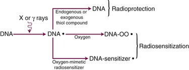
Although the exact mechanism(s) of the oxygen effect are likely complex, a fairly simplistic model can be used to illustrate our current understanding of this phenomenon (Fig. 1-22). The radical competition model holds that oxygen acts as a radiosensitizer by forming peroxides in important biomolecules (including, but not necessarily limited to, DNA) already damaged by radiation exposure, thereby “fixing” the radiation damage. In the absence of oxygen, DNA can be restored to its preirradiated condition by hydrogen donation from endogenous reducing species in the cell, such as the free radical scavenger glutathione (a thiol compound). In essence, this can be considered a type of very fast chemical restitution or repair. These two processes, fixation and restitution, are considered to be in a dynamic equilibrium, such that changes in the relative amounts of either the radiosensitizer, oxygen, or the radioprotector, glutathione, tip the scales in favor of either fixation (more damage, more cell killing, greater radiosensitivity) or restitution (less damage, less cell killing, greater radioresistance).
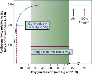
Consistent with this free radical-based interpretation of the oxygen effect is the finding that, for all intents and purposes, oxygen need only be present during the irradiation (or no more than about 5 ms after irradiation) to produce an aerobic radioresponse.110,111 The concentration of oxygen necessary to achieve maximum sensitization is quite small, evidence for the high efficiency of oxygen as a radiosensitizer. A sensitivity midway between a fully hypoxic and fully aerobic radioresponse is achieved at an oxygen tension of about 3 mm of mercury, corresponding to about 0.5% oxygen, more than a factor of 10 lower than partial pressures of oxygen usually encountered in normal tissues. This value of 0.5% has been termed oxygen’s “k-value” and is obtained from an oxygen “k-curve” of relative radiosensitivity plotted as a function of oxygen tension112 (Fig. 1-23).
Reoxygenation in Tumors
After the convincing demonstration of hypoxic cells in a mouse tumor,106 it was assumed that human tumors contained a viable hypoxic fraction as well. However, if human tumors contained even a small fraction of clonogenic hypoxic cells, simple calculations suggested that tumor control would be nearly impossible with radiation therapy.113 Because therapeutic successes obviously did occur, some form of reoxygenation must take place during the course of multifraction irradiation. This was not an unreasonable idea, because the demand for oxygen by sterilized cells would gradually decrease as such cells were removed from the tumor and a decrease in tumor size, a restructuring of tumor vasculature, or intermittent changes in blood flow could make oxygen available to these previously hypoxic cells.
The reoxygenation process was extensively studied by van Putten and Kallman,114 who serially determined the fraction of hypoxic cells in a mouse sarcoma during the course of a typical multifraction irradiation protocol. The fact that the hypoxic fraction was about the same at the end of treatment as at the beginning of treatment was strong evidence for a reoxygenation process. Reoxygenation of hypoxic, clonogenic tumor cells during an extended multifraction treatment would increase the therapeutic ratio, assuming that normal tissues remained well-oxygenated. This is thought to be another major factor in the sparing of normal tissues relative to tumors during fractionated radiation therapy.
What physiologic characteristics would lead to tumor reoxygenation during a course of radiotherapy, and at what rate would this be expected to occur? One possible cause of tumor hypoxia, and by extension, a possible mechanism for reoxygenation, was suggested by Thomlinson and Gray’s pioneering work.105 The type of hypoxia that they described is what is now called chronic hypoxia or diffusion-limited hypoxia. This results from the tendency of tumors to outgrow their blood supply, and given that oxygen is readily consumed by tumor cells, it follows that natural gradients of oxygen tension should develop as a function of distance from blood vessels. Cells situated beyond the diffusion distance of oxygen would be expected to be dead or dying, yet in regions of chronically low oxygen tension, clonogenic and radioresistant hypoxic cells may persist. Should the tumor shrink as a result of radiation therapy or if the cells killed by radiation have a decreased demand for oxygen, it is likely that this would allow some of the chronically hypoxic cells to reoxygenate. However, such a reoxygenation process could be quite slow—on the order of days or more—depending on how quickly tumors regress during treatment. The patterns of reoxygenation in some experimental rodent tumors are consistent with this mechanism of reoxygenation, but others are not.
Other rodent tumors reoxygenate very quickly, on a time scale of minutes to hours.115 This occurs in the absence of any measurable tumor shrinkage or change in oxygen utilization by tumor cells. In such cases, the model of chronic diffusion-limited hypoxia, and slow reoxygenation does not fit the experimental data. During the late 1970s, Brown and colleagues116 proposed that a second type of hypoxia may exist in tumors, an acute perfusion-limited hypoxia. Based on the growing understanding of the vascular physiology of tumors, it was clear that tumor vasculature was often abnormal in both structure and function secondary to abnormal angiogenesis. If tumor vessels were to close transiently from temporary blockage by blood cell components, vascular spasm, or high interstitial fluid pressure in the surrounding tissue, the tumor cells in the vicinity of those vessels would become acutely hypoxic almost immediately. Then, assuming blood flow resumed in minutes to hours, these cells would reoxygenate. However, this type of hypoxia can also occur in the absence of frank closure or blockage of tumor vessels, from, for example, vascular shunting or decreased red blood cell flux or overall blood flow rate.117 Because of this, the name “perfusion-limited” hypoxia is perhaps misleading; a better moniker might be “fluctuant” or “intermittent” hypoxia. Although intermittent hypoxia would explain the rapid reoxygenation observed for some tumors, it does not preclude the existence of chronic diffusion-limited hypoxia.
Intermittent hypoxia with rapid reoxygenation has since been demonstrated unambiguously for rodent tumors by Chaplin and colleagues.118 It is still not clear how many human tumors contain regions of hypoxia (although many do—see later discussion), what type(s) of hypoxia is present, whether this varies with tumor type or site, and whether and how rapidly reoxygenation occurs. However, the knowledge that tumor hypoxia is a diverse and dynamic process opens up a number of possibilities for the development of novel interventions designed to cope with, or even exploit, hypoxia.
Measurement of Hypoxia in Human Tumors
In 1988, one of the first studies showing a strong association between directly measured oxygenation status in tumors and clinical outcome was published by Gatenby.124 An oxygen-sensing electrode was inserted into the patient’s tumor, and multiple readings were taken at different depths along the probe’s track. The electrode was also repositioned in different regions of the tumor to assess intertrack variability in oxygen tension. Both the arithmetic mean PO2 value for a particular tumor as well as the tumor volume-weighted PO2 value directly correlated with local control rate. A high tumor oxygen tension was associated with a high complete response rate, and vice versa. In a similar, prospective study, Höckel and colleagues4,125 concluded that pretreatment tumor oxygenation was a strong predictor of outcome among patients with intermediate- and advanced-stage cervical carcinoma (Figure 1-24).
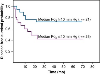
Today, oxygen electrodes are still considered the “gold standard” against which all other methods for measuring tumor oxygenation are compared. Unfortunately, the method has its limitations. One weakness is that relative to the size of individual tumor cells, the electrode is large, averaging an outer diameter of 300 µm, a tip recess of 120 µm, and a sampling volume of about 12 µm in diameter.126 Thus, not only is the oxygen tension measurement regional but the insertions and removals of the probe no doubt perturb the oxygenation status. Another problem is that there is no way to determine whether the tumor cells are viable or not. If such cells are hypoxic but not clonogenic, they would not be expected to affect the radiotherapy outcome.
A second direct technique for measuring oxygenation status takes advantage of a serendipitous finding concerning how hypoxic cell radiosensitizers are metabolized. Certain classes of radiosensitizers, including the nitroimidazoles, undergo a bioreductive metabolism in the absence of oxygen that leads to their becoming covalently bound to cellular macromolecules.127,128 Assuming that the bioreductively bound drug could be quantified by radioactive labeling129 or tagged with an isotope amenable to detection using positron emission tomography130 or magnetic resonance spectroscopy,131 a direct measure of hypoxic fraction can be obtained.
Another approach to detecting those cells containing bound drug was developed by Raleigh and colleagues.132,133 This immunohistochemical method involved the development of antibodies specific for the already-metabolized, bound nitroimidazoles. After injecting the parent drug, allowing time for the reductive metabolism to occur, and taking biopsies of the tumor and preparing histopathology slides, the specific antibody is applied to the slides and regions containing the bound drug are visualized directly. This immunostaining method has the distinct advantages that hypoxia can be studied at the level of individual tumor cells,134 spatial relationships between regions of hypoxia and other tumor physiologic parameters can be assessed,135 and the drug does not perturb the tumor microenvironment. However, the method remains an invasive procedure, is labor intensive, does not address the issue of the clonogenicity of stained cells (although such cells do have to be metabolically active), and requires that multiple samples be taken because of tumor heterogeneity.
One hypoxia marker based on the immunohistologic method, HypoxyProbe-1, is commercially available. It detects reductively-bound pimonidazole and has been used in experimental and clinical studies around the world.136,137 Applying HypoxyProbe-1 to human tumor specimens yields a range of hypoxic fractions similar to that noted for experimental rodent tumors and a mean value of approximately 15%.133,138 This marker can also be used to probe disease states other than cancer that may have the induction of tissue hypoxia as part of their etiology, such as cirrhosis of the liver139,140 and ischemia-reperfusion injury in the kidney.141
There is also considerable interest in endogenous markers of tissue hypoxia,142,143 which could reduce to some extent the procedural steps involved in, and the invasive aspects of, detecting hypoxia using exogenous agents. Among the endogenous cellular proteins being investigated in this regard are the hypoxia-inducible factor-1 alpha (HIF-1α, a transcription factor),144 the enzyme carbonic anhydrase IX (CA-9 or CAIX),145 glucose transporter-1 (GLUT-1),146–148 and osteopontin.149,150
Radiosensitizers, Radioprotectors, and Bioreductive Drugs
The perceived threat that tumor hypoxia posed spawned much research into ways of overcoming the hypoxia problem. One of the earliest proposed solutions was the use of high LET radiations,151 which were less dependent on oxygen for their biologic effectiveness. Other agents enlisted to deal with the hypoxia problem included hyperbaric oxygen breathing120; artificial blood substitutes with increased oxygen-carrying capacity152; oxygen-mimetic hypoxic cell radiosensitizers such as misonidazole or etanidazole122; hyperthermia153; normal tissue radioprotectors such as amifostine154; vasoactive agents thought to modify tumor blood flow such as nicotinamide155; agents that modify the oxygen-hemoglobin dissociation curve such as pentoxifylline156; and bioreductive drugs designed to be selectively toxic to hypoxic cells such as tirapazamine.157,158
Radiosensitizers
Radiosensitizers are loosely defined as chemical or pharmacologic agents that increase the cytotoxicity of ionizing radiation. “True” radiosensitizers meet the stricter criterion of being relatively nontoxic in and of themselves, acting only as potentiators of radiation toxicity. “Apparent” radiosensitizers still produce the net effect of making the tumor more radioresponsive, yet the mechanism is not necessarily synergistic nor is the agent necessarily nontoxic when given alone. Ideally, a radiosensitizer is only as good as it is selective for tumors. Agents that show little or no differential effect between tumors and normal tissues do not improve the therapeutic ratio and therefore may not be of much clinical utility. Table 1-2 summarizes some of the classes of radiosensitizers (and radioprotectors—discussed later) that have been used in the clinic.
TABLE 1-2 Selected Chemical Modifiers of Radiation Therapy
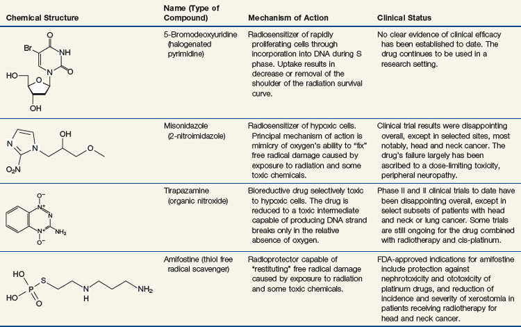
Hypoxic Cell Radiosensitizers
The increased radiosensitivity of cells in the presence of oxygen is believed to be due to oxygen’s affinity for the electrons produced by the ionization of biomolecules. Molecules other than oxygen also have this chemical property, known as “electron affinity,”159 including some agents that are not otherwise consumed by the cell. Assuming such an electron-affinic compound is not utilized by the cell, it should diffuse further from capillaries and reach hypoxic regions of a tumor and, acting in an oxygen-mimetic fashion, sensitize hypoxic cells to radiation.
One class of compounds that represented a realistic trade-off between sensitizer efficiency and diffusion effectiveness was the nitroimidazoles, which include such drugs as metronidazole, misonidazole, etanidazole, pimonidazole, and nimorazole. The nitroimidazoles consist of a nitroaromatic imidazole ring, a hydrocarbon side chain that determines the drug’s lipophilicity, and a nitro group that determines the drug’s electron affinity. Misonidazole was extensively characterized in cellular and animal model systems, culminating in its use in clinical trials. Clinical experiences with misonidazole and some of its successor compounds are discussed in Chapter 7.
Unfortunately, the nitroimidazoles also have characteristics that decrease their clinical usefulness. The hydrocarbon side chain of the molecule determines its lipophilicity, and this chemical property affects the drug’s pharmacokinetic action, which is a primary determinant of drug-induced side effects.160 The dose-limiting toxicity of the fairly lipophilic agent misonidazole is peripheral neuropathy, an unanticipated and serious side effect.122,161 Etanidazole was specifically designed to be less lipophilic162 in the hopes of decreasing the neurologic toxicity. Although this goal was accomplished as a proof of concept, clinical results with etanidazole were otherwise disappointing163 (see also Chapter 7).
Finally, considering the prodigious amount of research and clinical effort that has gone into the investigation of hypoxic cell radiosensitizers over the past 45 years, it is difficult not to be discouraged by the predominantly negative results of the clinical trials. However, these negative results have prompted a rethinking of the hypoxia problem and novel approaches to dealing with it, as well as consideration of other factors that may have contributed to the lack of success of the nitroimidazole radiosensitizers.161 The following are among the more obvious questions raised:
Proliferating Cell Radiosensitizers
Analogs of the DNA precursor thymidine, such as bromodeoxyuridine (BrdUdR) or iododeoxyuridine (IdUdR), can be incorporated into the DNA of actively proliferating cells in place of thymidine because of close structural similarities between the compounds. Cells containing DNA substituted with these halogenated pyrimidines are more radiosensitive than normal cells, with the amount of sensitization directly proportional to the fraction of thymidine replaced.164 In general, the radiosensitization takes the form of a decrease in or elimination of the shoulder region of the radiation survival curve. To be maximally effective, the drug must be present for at least several rounds of DNA replication prior to irradiation. Although the mechanism by which BrdUdR and IdUdR exert their radiosensitizing effect remains somewhat unclear, it is likely that both the formation of more complex radiation-induced lesions in the vicinity of the halogenated pyrimidine molecules and the interference with DNA damage sensing or repair are involved.165
The clinical use of halogenated pyrimidines began in the late 1960s, with a major clinical trial in head and neck cancer.166 In retrospect, the choice of head and neck tumors for this study was far from ideal, because the oral mucosa is also a rapidly proliferating tissue and was similarly radiosensitized, causing severe mucositis, and the therapeutic ratio overall was poor. In later years, tumors selected for therapy with halogenated pyrimidines were chosen in the hopes of maximizing the differential radiosensitization between tumors and normal tissues.167 Aggressively growing tumors surrounded by slowly-proliferating or nonproliferating normal tissues, such as high-grade brain tumors or some sarcomas, have been targeted for example.168,169 Later strategies for further improving radiosensitization by BrdUdR and IdUdR involved changing the schedule of drug delivery: giving the drug as a long, continuous infusion both before and during radiotherapy170; and administering the drug as a series of short, repeated exposures.171
Bioreductive Drugs
In the wake of the failure of most hypoxic cell radiosensitizers to live up to their clinical potential, a new approach to combating the hypoxia problem emerged: the use of bioreductive drugs that are selectively toxic to hypoxic cells. Although these agents kill rather than sensitize hypoxic cells, the net effect of combining them with radiation therapy is apparent sensitization of the tumor due to the elimination of an otherwise radioresistant subpopulation. Such drugs have been shown to outperform the nitroimidazole radiosensitizers in experimental studies with clinically relevant fractionated radiotherapy.172 To the extent that hypoxic cells are also resistant to chemotherapy because of tumor microenvironmental differences in drug delivery, pH, or the cell’s proliferative status, complementary tumor cell killing might be anticipated for combinations of bioreductive agents and anticancer drugs as well.173
Most hypoxia-specific cytotoxic drugs fall into three categories: the nitroheterocyclics, the quinone antibiotics. and the organic nitroxides.174 All require bioreductive activation by nitroreductase enzymes such as cytochrome P450, DT-diaphorase, and nitric oxide synthase, to reduce the parent compound to its cytotoxic intermediate, typically an oxidizing free radical capable of damaging DNA and other cellular macromolecules. The active species is either not formed or else is immediately back-oxidized to the parent compound in the presence of oxygen, which accounts for its preferential toxicity under hypoxic conditions. Examples of nitroheterocyclic drugs with bioreductive activity include misonidazole and etanidazole175,176 and dual-function agents such as RSU 1069.177 The latter drug is termed “dual function” because its bioreduction also activates a bifunctional alkylating moiety capable of introducing crosslinks into DNA. Mitomycin C and several of its analogs (including porfiromycin and EO9) are quinones with bioreductive activity that have been tested in randomized clinical trials in head and neck tumors.178
The lead compound for the third class of bioreductive drugs, the organic nitroxides, is tirapazamine (SR 4233)157,158,172 (see Table 1-2). The dose-limiting toxicity for single doses of tirapazamine is a reversible hearing loss; other effects observed include nausea and vomiting and muscle cramps.179
Tirapazamine is particularly attractive because it both retains its hypoxia-selective toxicity over a broader range of (low) oxygen concentrations than the quinones and nitroheterocyclic compounds180 and its “hypoxic cytotoxicity ratio,” the ratio of drug doses under hypoxic versus aerobic conditions to yield the same amount of cell killing, averages an order of magnitude higher than for the other classes of bioreductive drugs.173 Laboratory and clinical data also support a tumor-sensitizing role for tirapazamine in combination with the chemotherapy agent cisplatinum.179
To date, randomized phase II and III clinical trials with tirapazamine combined with radiotherapy and/or chemotherapy (particularly, cisplatinum) have yielded mixed results.179,181 Although the drug has in no way become a staple of clinical practice, its activity against some tumors warrants further investigation, as does the search for more effective agents from the same or a similar chemical class.
Normal Tissue Radioprotectors
Amifostine (WR 2721) (see Table 1-2) is a phosphorothioate compound developed by the United States Army for use as a radiation protector. Modeled after naturally occurring radioprotective sulfhydryl compounds such as cysteine, cysteamine, and glutathione,182 amifostine’s mechanism of action involves the scavenging of free radicals produced by ionizing radiation, radicals that otherwise could react with oxygen and “fix” the chemical damage. Amifostine can also detoxify other reactive species through the formation of thioether conjugates, and, in part because of this, the drug can also be used as a chemoprotective agent.183 Amifostine is a pro-drug that is dephosphorylated by plasma membrane alkaline phosphatase to the free thiol WR 1065, the active metabolite. As is the case with the hypoxic cell radiosensitizers, amifostine need only be present at the time of irradiation to exert its radioprotective effect.
In theory, if normal tissues could be made to tolerate higher total doses of radiation through the use of radioprotectors, then the relative radioresistance of hypoxic tumor cells would be negated. However, encouraging preclinical studies demonstrating radioprotection of a variety of cells and tissues notwithstanding,184,185 radioprotectors such as amifostine would not be expected to increase the therapeutic ratio unless they could be introduced selectively into normal tissues but not tumors. The pioneering studies of Yuhas and colleagues154,186,187 addressed this issue by showing that the drug’s active metabolite reached a higher concentration in most normal tissues than in tumors and that this mirrored the extent of radioprotection or chemoprotection. The selective protection of normal tissues apparently results from tumors being both less able to convert amifostine to WR 1065 (because of lower concentrations of the required phosphatases) and to transport this active metabolite throughout the cell.
Dose-reduction factors (DRFs) (the ratio of radiation doses to produce an isoeffect in the presence versus the absence of the radioprotector) in the range of 1.5 to 3.5 are achieved for normal tissues, whereas the corresponding DRFs for tumors seldom exceed 1.2. Those normal tissues exhibiting the highest DRFs include bone marrow and gastrointestinal tract, liver, testicular, and salivary gland tissues.154 Brain and spinal cord tissues are not protected by amifostine, and the oral mucosa is only marginally protected.154 Comparable protection factors are obtained for some chemotherapy agents, including cyclophosphamide and cisplatin.188,189 The dose-limiting toxicities associated with the use of amifostine include hypotension, emesis, and generalized weakness or fatigue.190
Finally, just as there are apparent radiosensitizers there are also apparent radioprotectors that have the net effect of allowing normal tissues to better tolerate higher doses of radiation and chemotherapy but through mechanisms of action not directly related to the scavenging of free radicals. Various biologic response modifiers, including cytokines, prostaglandins (such as misoprostol),191,192 anticoagulants (such as pentoxifylline)193,194 and protease inhibitors are apparent radioprotectors because they can interfere with the chain of events that normally follows the killing of cells in tissues by, for example, stimulating compensatory repopulation or preventing the development of fibrosis. Finally, there is also growing interest in the use of biologic agents that inhibit apoptosis as normal tissue radioprotectors.195,196 Such agents have little or no effect on tumor cells, most of which are already apoptosis-resistant.
[/level-membership-for-hematology-oncology-and-palliative-medicine-category][not-level-membership-for-hematology-oncology-and-palliative-medicine-category]
Chapter 1 Biologic Basis of Radiation Oncology
What Is Radiation Biology?
Most of this chapter will be devoted to so-called classical radiobiology, that is, studies that largely predate the revolution in molecular biology of the 1980s and 1990s. Although the reader might be tempted to view this body of knowledge as rather primitive by today’s standards, relying too heavily on phenomenology, empiricism, and simplistic, descriptive models and theories, the real challenge is to integrate the new biology into the already-existing framework of classical radiobiology; this will be discussed in detail in Chapter 2.
Radiotherapy-Oriented Radiobiology: A Conceptual Framework
Therapeutic Ratio
The concept of therapeutic ratio is best illustrated graphically, by making a direct comparison of dose-response curves for both tumor control and normal tissue complication rates plotted as a function of dose. Examples of this approach are shown in Figure 1-1, for cases in which the therapeutic ratio is either “unfavorable,” “favorable,” or “optimal,” bearing in mind that these are theoretical curves. Actual dose-response curves derived from experimental or clinical data are much more variable, particularly for tumors, which tend to show much shallower dose responses.1 This serves to underscore how difficult it can be in practice to assign a single numerical value to the therapeutic ratio in any given situation.
Radiation Biology “Continuum”
There is a surprising continuity between the physical events that occur in the first picosecond (or less) after ionizing radiation interacts with biologic material and the ultimate consequences of that interaction on tissues. The consequences themselves may not become apparent until days, weeks, months, or even years after the radiation exposure. Some of the important steps in this radiobiology “continuum” are listed in Table 1-1. The orderly progression from one stage of the continuum to the next—from physical to physicochemical to biochemical to biologic—is particularly noteworthy not only because of the vastly different time scales over which the critical events occur, but also because of the increasing biologic complexity associated with each of the endpoints or outcomes. Each stage of the continuum also offers a unique radiobiologic window of opportunity: the potential to intervene in the process and thereby modify all the events and outcomes that follow.
Tissue Heterogeneity
Normal tissues, being composed of more than one type of cell, are somewhat heterogeneous, and tumors, owing both to the genetic instability of individual tumor cells and to microenvironmental differences, are very heterogeneous. Different subpopulations of cells have been isolated from many types of human and experimental cancers, and these may differ in antigenicity, metastatic potential, sensitivity to radiation therapy and chemotherapy, and so on.2,3 This heterogeneity is manifest within a particular patient, and to a much greater extent, between patients with otherwise similar tumors.
What are the practical implications of normal tissue and tumor heterogeneity? First, if one assumes that normal tissues are the more uniform and predictable in behavior of the two, then tumor heterogeneity is responsible, either directly or indirectly, for most radiotherapy failures. If so, this suggests that a valid clinical strategy might be to identify the radioresistant subpopulation(s) of tumor cells and then tailor therapy specifically to cope with them. This approach is much easier said than done. Some prospective clinical studies now include one or more pretreatment determinations of, for example, the extent of tumor hypoxia4 or the potential doubling time of tumor clonogens5 as criteria for assigning patients to different treatment groups.
“Powers of Ten”
The tumor control probability for a given fraction of surviving cells is not particularly helpful if the total number of cells at risk is unknown, however, and this is where an understanding of logarithmic relationships and exponential cell killing is useful. Based on the resolution of existing tools and technology for cancer detection, let us assume that a 1-cm3 (1-g) tumor mass can be identified reliably. A tumor of this size has been estimated to contain approximately 109 cells,6 admittedly a theoretical value that assumes all cells are perfectly “packed” and uniformly sized and that the tumor contains no stroma. A further assumption, that all such cells are clonogenic (rarely, if ever, the case), suggests that at least 9 logs of cell killing would be necessary before any appreciable tumor control (about 37%) would be achieved, and 10 logs of cell killing would be required for a high degree of tumor control (i.e., 90%).
After the first log or two of cell killing, however, some tumors respond by shrinking, a partial response. After two to three logs of cell killing, the tumor may shrink to a size below the current limits of clinical detection, that is, a complete response. Although partial and complete responses are valid clinical endpoints, a complete response does not necessarily mean tumor cure. At least six more logs of cell killing would be required before any significant probability of cure would be expected. This explains why radiation therapy is not halted if the tumor “disappears” during the course of treatment; this concept is illustrated graphically in Figure 1-2.
Radiation Biology and Therapy: The First 50 Years
In less than 4 years after the discovery of x rays by Roentgen,7 radioactivity by Becquerel,8 and radium by the Curies,9 the new modality of cancer treatment known as radiation therapy claimed its first apparent cure of skin cancer.10 Today, more than a century later, radiotherapy is most commonly given as a series of small daily dose fractions of approximately 1.8 to 2 Gy each, 5 days per week, over a period of 5 to 7 weeks, to a total dose of 50 to 70 Gy. Although it is true that the historical development of this conventional radiotherapy schedule was empirically based, there were a number of early radiobiologic experiments that suggested this approach.
In the earliest days of radiotherapy, both x rays and radium were used for cancer treatment. Because of the greater availability and convenience of using x-ray tubes and the higher intensities of radiation output achievable, it was fairly easy to deliver large single doses in short overall treatment times. Thus, from about 1900 into the 1920s, this “massive dose technique”11 was a common way of administering radiation therapy. Unfortunately, normal tissue complications were quite severe. To make matters worse, the rate of local tumor recurrence was still unacceptably high.
As early as 1906, Bergonié and Tribondeau12 observed histologically that the immature dividing cells of the rat testis showed evidence of damage at lower radiation doses than the mature nondividing cells. Based on these observations, the two researchers put forth some basic “laws” stating that x rays were more effective on cells that were: (1) actively dividing, (2) likely to continue to divide indefinitely, and (3) poorly differentiated.12 Because tumors were already known to contain cells that not only were less differentiated but also exhibited greater mitotic activity, Bergonié and Tribondeau reasoned that several radiation exposures might preferentially kill these tumor cells but not their slowly proliferating, differentiated counterparts in the surrounding normal tissues.
The end of common usage of the single-dose technique in favor of fractionated treatment came during the 1920s as a consequence of the pioneering experiments of Claude Regaud and colleagues.13 Using the testis of the rabbit as a model tumor system (because the rapid and unlimited proliferation of spermatogenic cells simulated to some extent the pattern of cell proliferation in malignant tumors), Regaud14 showed that only through the use of multiple radiation exposures could animals be completely sterilized without producing severe injury to the scrotum. Regaud15 suggested that the superior results afforded the multifraction irradiation scheme were related to alternating periods of relative radioresistance and sensitivity in the rapidly proliferating germ cells. These principles were soon tested in the clinic by Henri Coutard,16,17 who used fractionated radiotherapy for the treatment of head and neck cancers, with spectacularly improved results. Mainly as a result of these and related experiments, fractionated treatment subsequently became the standard form of radiation therapy.
Time-dose equivalents for skin erythema published by Reisner,18 Quimby and MacComb,19 and others20,21 formed the basis for the calculation of equivalents for other tissue and tumor responses. By plotting the total doses required for each of these “equivalents” for a given level of effect in a particular tissue, as a function of a treatment parameter such as overall treatment time, number of fractions, dose per fraction, and so on, an isoeffect curve could be derived. All time-dose combinations that fell along such a curve would, theoretically, produce tissue responses of equal magnitude. Isoeffect curves, relating the total dose to the overall treatment time, derived in later years from some of these data,22 are shown in Figure 1-3.
Figure 1-3 Isoeffect curves relating the log of the total dose to the log of the overall treatment time for various levels of skin reaction and the cure of skin cancer. A, Isoeffect curves were constructed by Cohen on the basis of a survey of earlier published data on radiotherapy equivalents.21–26 The slope of the curves for skin complications was 0.33, and the slope for tumor control was 0.22. B, The Strandqvist28 isoeffect curves were first published in 1944. All lines were drawn parallel and had a common slope of 0.33.
A, Adapted from Cohen L: Radiation response and recovery: Radiobiological principles and their relation to clinical practice. In Schwartz E, editor: The Biological Basis of Radiation Therapy, Philadelphia, 1966, JB Lippincott, p 208; B, adapted from Strandqvist M: Studien uber die kumulative Wirkung der Roentgenstrahlen bei Fraktionierung, Acta Radiol Suppl 55:1, 1944.
The first published isoeffect curves were produced by Strandqvist23 in 1944, and are also shown in Figure 1-3. When transformed on log-log coordinates, isoeffect curves for a variety of skin reactions, and the cure of skin cancer, were drawn as parallel lines, with common slopes of 0.33. These results implied that there would be no therapeutic advantage to using prolonged treatment times (i.e., multiple small fractions versus one or a few large doses) for the preferential eradication of tumors while simultaneously sparing normal tissues.24 It was somewhat ironic that the Strandqvist curves were so popular in the years that followed, when it was already known that the therapeutic ratio did increase (at least to a point) with prolonged, as opposed to very short, overall treatment times. However, the overarching advantage was that these isoeffect curves were quite reliable at predicting skin reactions, which were the dose-limiting factors at that time.
The “Golden Age” of Radiation Biology and Therapy: The Second 50 Years
Perhaps the defining event that ushered in the golden age of radiation biology was the publication of the first survival curve for mammalian cells exposed to graded doses of ionizing radiation.25 This first report of a quantitative measure of intrinsic radiosensitivity of a human cell line (HeLa, derived from a cervical carcinoma26) was published by Puck and Marcus25 in 1956. To put this seminal work in the proper perspective, however, it is first necessary to review the physicochemical basis for why ionizing radiation is toxic to biologic materials.
The Interaction of Ionizing Radiation with Biologic Materials
As mentioned in the introductory section of this chapter, ionizing radiation deposits energy as it traverses the absorbing medium through which it passes. The most important feature of the interaction of ionizing radiation with biologic materials is the random and discrete nature of the energy deposition. Energy is deposited in increasingly energetic packets referred to as “spurs” (100 eV or less deposited), “blobs” (100 to 500 eV), or “short tracks” (500 to 5000 eV), each of which can leave from approximately three to several dozen ionized atoms in its wake. This is illustrated in Figure 1-4, along with a segment of (interphase) chromatin shown to scale. The frequency distribution and density of the different types of energy deposition events along the track of the incident photon or particle are measures of the radiation’s linear energy transfer or LET (see also the “Relative Biologic Effectiveness” section, later). Because these energy deposition events are discrete, it follows that although the average amount of energy deposited in a macroscopic volume of biologic material may be rather modest, the distribution of this energy on a microscopic scale may be quite large. This explains why ionizing radiation is so efficient at producing biologic damage; the total amount of energy deposited in a 70-kg human that will result in a 50% probability of death is only about 70 calories, about as much energy as is absorbed by drinking one sip of hot coffee.27 The key difference is that the energy contained in the sip of coffee is uniformly distributed, not random and discrete.
Any and all cellular molecules are potential targets for the localized energy deposition events that occur in spurs, blobs, or short tracks. Whether the ionization of a particular biomolecule results in a measurable biologic effect depends on a number of factors, including how probable a target the molecule represents from the point of view of the ionizing particle, how important the molecule is to the continued health of the cell, how many copies of the molecule are normally present in the cell and to what extent the cell can react to the loss of “working copies,” and how important the cell is to the structure or function of its corresponding tissue or organ. DNA, for example, is obviously an important cellular macromolecule and one that is present only as a single double-stranded copy. On the other hand, other molecules in the cell may be less crucial to survival yet are much more abundant than DNA, and therefore have a much higher probability of being hit and ionized. The most abundant molecule in the cell by far is water, comprising some 80% to 90% of the cell on a per weight basis. The highly reactive free radicals formed by the radiolysis of water are capable of adding to the DNA damage resulting from direct energy absorption by migrating to the DNA and damaging it indirectly. This mechanism is referred to as “indirect radiation action” to distinguish it from the aforementioned “direct radiation action.”28 The direct and indirect action pathways for ionizing radiation are illustrated below.
The most highly reactive and damaging species produced by the radiolysis of water is the hydroxyl radical (•OH), although other free radical species are also produced in varying yields.29,30 Ultimately, it has been determined that cell killing by indirect action constitutes some 70% of the total damage produced in DNA for low LET radiation.
The •OH radical is capable of both abstraction of hydrogen atoms from other molecules and addition across carbon-carbon or other double bonds. More complex macromolecules that have been converted to free radicals can undergo a series of transmutations in an attempt to rid themselves of unpaired electrons, many of which result in the breakage of nearby chemical bonds. In the case of DNA, these broken bonds may result in the loss of a base or an entire nucleotide or in frank scission of the sugar phosphate backbone, involving one or both DNA strands. In some cases, chemical bonds are first broken but then rearranged, exchanged, or rejoined in inappropriate ways. Bases in DNA may be modified by the addition of one or more hydroxyl groups (e.g., the base thymine converted to thymine glycol), pyrimidines may become dimerized, and/or the DNA may become cross-linked to itself or to associated protein components. And again, because the initial energy deposition events are discrete, the free radicals produced also are clustered and therefore undergo their multiple chemical reactions and produce multiple damages in a highly localized area. This has been termed the “multiply-damaged site”31 or “cluster”32 hypothesis. Examples of the types of damage found in irradiated DNA are shown in Figure 1-5.
Biochemical Repair of DNA Damage
The study of DNA repair in mammalian cells received a significant boost during the late 1960s with publications by Cleaver33,34 that identified the molecular defect responsible for the human disease xeroderma pigmentosum (XP). Patients with XP are exquisitely sensitive to sunlight and highly cancer-prone (particularly to skin cancers). Cleaver showed that cells derived from such patients were likewise sensitive to UV radiation and defective in the nucleotide excision repair pathway (discussed later). These cells were not especially sensitive to ionizing radiation, however. Several years later, Taylor and colleagues35 reported that cells derived from patients with a second cancer-prone disorder called ataxia telangiectasia (AT) were extremely sensitive to ionizing radiation and radiation-mimetic drugs but not to UV radiation. In the years that followed, cell cultures derived from patients with these two conditions were used to help elucidate the complicated processes of DNA repair in mammalian cells.
Today, many rodent and human genes involved in DNA repair have been cloned.36 Nearly 20 distinct gene products participate in excision repair of base damage, and even more are involved in the repair of strand breaks. Many of these proteins function as component parts of larger repair complexes; some of these parts are interchangeable and participate in other DNA repair and replication pathways as well. It is also noteworthy that some are not involved with the repair process per se but rather link DNA repair to other cellular functions, including transcription, cell cycle arrest, chromatin remodeling, and apoptosis.37 This attests to the fact that the maintenance of genomic integrity results from a complex interplay between not only the repair proteins themselves but between others that serve as damage sensors, signaling mediators and transducers, and effectors.
For example, the defect responsible for the disease AT is not in a gene that codes for a repair protein but rather in a gene that participates in damage recognition and in a related pathway that normally prevents cells from entering S phase of the cell cycle and beginning DNA synthesis while residual DNA damage is present. This was termed the G1/S checkpoint response.38 Because of this genetic defect, AT cells do not experience the normal G1 arrest after irradiation and enter S phase with residual DNA damage. This accounts both for the exquisite radiosensitivity of AT cells and the resulting genomic instability that can lead to carcinogenesis.
What is known about the various types of DNA repair in mammalian cells is outlined below.
Base Excision Repair
The repair of base damage is initiated by DNA repair enzymes called DNA glycosylases, which recognize specific types of damaged bases and excise them without otherwise disturbing the DNA strand.39 The action of the glycosylase itself results in the formation of another type of damage observed in irradiated DNA—an apurinic or apyrimidinic (AP) site. The AP site is then recognized by another repair enzyme, an AP endonuclease, which nicks the DNA adjacent to the lesion. The resulting strand break becomes the substrate for an exonuclease, which removes the abasic site, along with a few additional bases. The small gap that results is patched by DNA polymerase, which uses the opposite, hopefully undamaged, DNA strand as a template. Finally, DNA ligase seals the patch in place.
Nucleotide Excision Repair
The DNA glycosylases that begin the process of base excision repair do not recognize all known forms of base damage, however, particularly bulky or complex lesions.39 In such cases, another group of enzymes, termed structure-specific endonucleases, initiate the excision repair process. These repair proteins do not recognize the specific lesion but are thought instead to recognize more generalized structural distortions in DNA that necessarily accompany a complex base lesion. The structure-specific endonucleases incise the affected DNA strand on both sides of the lesion, releasing an oligonucleotide fragment made up of the damage site and several bases on either side of it. Because a longer segment of excised DNA—including both bases and the sugar phosphate backbone—is generated, this type of excision repair is referred to as nucleotide excision repair to distinguish it from base excision repair (described earlier), where the initial step in the repair process is removal of the damaged base only. After this step, the remainder of the nucleotide excision repair process is similar to that of base excision repair; the gap is then filled in by DNA polymerase and sealed by DNA ligase. Overall, however, nucleotide excision repair is a much slower process, with a half-time of approximately 12 hours.
For both types of excision repair, active genes in the process of transcription are repaired preferentially and more quickly. This has been termed transcription-coupled repair.40
Strand Break Repair
Despite the fact that unrepaired or mis-rejoined strand breaks, particularly DSBs, often have the most catastrophic consequences for the cell in terms of loss of reproductive integrity,41 the way in which mammalian cells repair strand breaks has been more difficult to elucidate than the way in which they repair base damage. Much of what was originally discovered about these repair processes is derived from studies of x ray–sensitive rodent cells and microorganisms that were subsequently discovered to harbor specific defects in strand break repair. Since then, other human genetic diseases characterized by DNA repair defects have been identified and are also used to help probe these fundamental processes.
A genetic technique known as complementation analysis allows further characterization of genes involved in DNA repair. Complementation analysis involves the fusion of different strains of cells possessing the same phenotypic defect and subsequent testing of the hybrid cell for the presence or absence of this phenotype. Should two cell types bearing the defect yield a phenotypically normal hybrid cell, this implies that the defect has been “complemented” and that the defective phenotype must result from mutations in at least two different genes. With respect to DNA strand break repair, eight different genetic complementation groups have been identified in rodent cell mutants. For example, a mutant Chinese hamster cell line, designated EM9, seems especially radiosensitive owing to delayed repair of DNA single-strand breaks, a process that is normally complete within minutes of irradiation.42
With respect to the repair of DNA DSBs, the situation is more complicated in that the damage on each strand of DNA may be different, and, therefore, no intact template would be available to guide the repair process. Under these circumstances, cells depend on genetic recombination (nonhomologous end joining or homologous recombination43) to cope with the damage.
The BRCA1 and BRCA2 gene products are also implicated in HR (and, possibly, NHEJ as well) because they interact with the Rad51 protein. Defects in these genes are associated with hereditary breast and ovarian cancer.44
Mismatch Repair
The primary role of mismatch repair (MMR) is to eliminate from newly synthesized DNA errors such as base/base mismatches and insertion/deletion loops caused by DNA polymerase.45 Descriptively, this process consists of three steps: mismatch recognition and assembly of the repair complex, degradation of the error-containing strand, and repair synthesis. In humans, MMR involves at least five proteins, including hMSH2, hMSH3, hMSH6, hMLH1, and hPMS2, as well as other members of the DNA repair and replication machinery.
One manifestation of a defect in mismatch repair is microsatellite instability, mutations observed in DNA segments containing repeated sequence motifs.46 Collectively, this causes the cell to assume a hypermutable state (“mutator phenotype”) that has been associated with certain cancer predisposition syndromes, in particular, hereditary nonpolyposis colon cancer (HNPCC, sometimes called Lynch syndrome).47,48
Cytogenetic Effects of Ionizing Radiation
Most chromosome aberrations result from an interaction between two (or more; discussed later) damage sites, and, therefore, can be grouped into three different types of “exchange” categories. A fourth category is reserved for chromosome aberrations thought to result from a single damage site.49 These categories are described below, and representative types of aberrations from each category are shown in Figure 1-6:
These four categories can be further subdivided according to whether the initial radiation damage occurred before or after the DNA is replicated during S phase of the cell cycle (a chromosome-type vs. a chromatid-type of aberration, respectively) and, for the three exchange categories, whether the lesion interaction was symmetric or asymmetric. Asymmetric exchanges always lead to the formation of acentric fragments that are usually lost in subsequent cell divisions and therefore are nearly always fatal to the cell. These fragments may be retained transiently in the cell’s progeny as extranuclear chromatin bodies called micronuclei. Symmetric exchanges are more insidious in that they do not lead to the formation of acentric fragments and the accompanying loss of genetic material at the next cell division, they are sometimes difficult to detect cytologically, and they are not invariably lethal to the cell. As such, they will be transmitted to all the progeny of the original cell. Some types of symmetric exchanges (a reciprocal translocation, for example) have been implicated in radiation carcinogenesis, insofar as they have the net effect of either bringing new combinations of genes together or of separating preexisting groups of genes.27 Depending on where in the genome the translocation takes place, genes normally on could be turned off, or vice versa, possibly with adverse consequences.
[/not-level-membership-for-hematology-oncology-and-palliative-medicine-category]
