INTRODUCTION

Most meningiomas are slowly growing lesions that can occur on the surface of the brain, the skull base, the dural reflections, or within the ventricles. About 90% of these tumors are classified as benign.¹ Neurosurgeons generally avoid operating on patients with small meningiomas, particularly those that are difficult to access surgically, and prefer to carefully monitor tumor growth.² Monitoring includes neurologic evaluation and periodically acquiring magnetic resonance scans of the patient’s brain. Neuroradiologists and clinicians visually inspect the scans for evidence of tumor growth. In clinical practice, finding evidence for subtle growth can be very difficult, particularly between scans taken at relatively short intervals. The main reason for the difficulty is that any changes in the head position or variations in the intensity profile between scans can actually obscure the slow growth that is so characteristic of meningiomas. In addition, very small changes in the linear dimensions seen on cross-sectional imaging can reflect appreciable volumetric change.

In this chapter, we first review common procedures for measuring tumor growth. We then describe a software tool that is specifically targeted toward detecting the evolution of meningiomas. Further, we test the tool on magnetic resonance images (MRI) acquired in standard clinical settings.

COMMON PROCEDURES FOR MEASURING TUMOR GROWTH

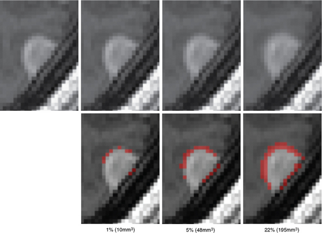
Surgeons and oncologists frequently analyze the evolution of tumors by viewing brain scans via a light box or visualization software. The analysis often includes sophisticated measuring techniques, as simple visual inspections of the images typically ignore small tumor growth (Fig. 17-1). These techniques commonly measure the size of the tumor individually for each scan, then compute the growth by combining the measurements of consecutive scans. Because change in the tumor dimension may be so difficult to appreciate between any two sequential scans it becomes critical that the clinician compare the most recent scan to the earliest available image as only by comparing these may the growth of the tumor be visibly evident (see Fig. 17-1 for an example). Thus, the patient may undergo extra testing and tumor growth may not be promptly detected. In addition, such methods do not provide a quantitative measure that could give an indication of the rate of growth and thus aid in treatment decisions. One metric for performing this task is the World Health Organization (WHO) response criteria.³ The criteria infer the size of each tumor through bidimensional measurements, which are the tumor’s largest diameter and perpendicular diameter.⁴ To increase efficiency and reproducibility, the Response Evaluation Criteria in Solid Tumors (RECIST)⁵ is based only on the largest diameter. However, both measurements ignore small growth deviating from the largest diameter directions.^6,7 More accurate measures have come from manual segmentations of the tumor volume, but these approaches are very labor intensive, and are sensitive to large variations in experts identifying tumor regions.⁸ To streamline the process, researchers have developed automatic methods.^9,10 These methods generally outline pathology by combining the image data with general information about the visual appearance of healthy tissue and pathology. The automatic methods are, however, still impacted by intrarater variability caused by image artifacts or altered head position, as they determine the tumor volume separately for each scan. To date, there has not been a technique that has been widely adopted by clinicians.

FIGURE 17-1 The real scan of the patient with synthetically evolving pathology of 1%, 5%, and 22% volume growth (shown in red in the second row). Visually detecting growths of 1% and 5% is extremely difficult.

In recent years, a new line of automatic tools has emerged that analyzes growth of lesions by processing a sequence of scans simultaneously.^11–13 These tools first normalize the sequence of images and then relate unusual patterns across the scans to regions of change. In this spirit, Rey and colleagues¹⁴ aligned the series of scans of multiple sclerosis patients to each other, a process that resulted in a deformation map that defined region-specific transformations from one scan to the next. They then showed that growing lesions produce patterns in the maps that are inherently different from dormant tissue. Angelini and colleagues¹⁵ proposed an alternative approach for brain tumors in which expected variations across the scan due to magnetic resonance acquisition were accounted for by aligning the head in each scan to a fixed pose and equalizing the global intensity patterns across the scans. They then related gross regional differences in intensity patterns across the scans to tumor growth.

To the best of our knowledge, state-of-the-art software tools are tested on scans with visible tumor/lesion growth only, as was the case for Rey¹⁴ and Angelini and colleagues.¹⁵ To address this gap, in the remainder of this chapter, we describe a semi-automatic procedure specifically targeted toward identifying difficult-to-detect changes in pathology. The software is easy to calibrate and, in less than 5 minutes, returns the total area of tumor change in cubic millimeters. We tested the tool on post-gadolinium, T1-weighted MRI acquired via a standard clinical acquisition sequence. This approach has been disseminated as part of the 3D Slicer (www.slicer.org), a publicly available software package targeted toward medical imaging processing and visualization.

A SOFTWARE TOOL FOR MONITORING SLOWLY GROWING TUMORS

Our software pipeline detects subtle changes in pathology at the level of a few voxels in three steps. The tool identifies the tumor in the first scan, then normalizes the series of scans, and finally detects growth based on the previous results.

The first step semi-automatically detects the tumor in the first scan. At this point, the method processes only the first scan, avoiding issues of intrarater variability. Further, we require manual supervision of the segmentation process to ensure the accuracy of the results. The user specifies a region of interest in the tumor and a lower bound on the intensities characterizing the pathology. From this input, the pipeline reliably extracts most of the pathology from post-gadolinium, T1-weighted MRIs, as meningiomas are generally characterized as homogeneous, bright objects.¹⁶ The software then removes small islands and holes caused by noise in the MRIs from the resulting binary map. We note that the resulting map will also include part of the dura, vessels, and skull because these structures have intensity patterns similar to pathology (Fig. 17-2). Because these structures are dormant, however, they should not substantially impact the analysis.

FIGURE 17-2 The top row shows images related to the first scan and the bottom row to the second scan. The first column consists of the input of the pipeline. The second column is the result of the second step of the pipeline. The top right shows the outcome of the semi-automatic segmentation of the image to the left. The bottom right is the outcome of the analysis with red indicating areas of growth.

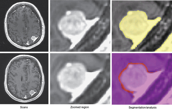
The second step automatically aligns the pathology of the remaining scan to the first. It does so by registering the scans to a common reference frame.¹⁷ The (rigid) registration only adjusts the global pose of each scan, preserving the size of the tumor. Now, the tumor regions across all scans are roughly aligned with each other so that the previously assigned region of interest defines the tumor region across all scans. The method then increases the resolution within each region to address partial voluming effects in the MRIs. Partial voluming artifacts are caused by insufficient image resolution leading to multiple structures within a voxel. Tissue boundaries then often become blurry as the intensity of these voxels is correlated to combinations of intensities of the adjacent structures. Finally, the framework addresses non-linear perturbation artifacts by repeating the initial alignment procedure and focusing only on the tumor regions. This process results in a series of images where, in theory, barring temporal changes, the pathology is well aligned (see second column of Fig. 17-2).

The final step of the pipeline measures the evolution of the tumor via two metrics. Motivated by Angelini and colleagues,¹⁵ the first metric detects change via analyzing differences in local intensity patterns. It does so by first mapping the segmentation of this first scan to the reference framework defined by the second step. The method then infers from the segmentation a conservative estimate of dormant tissue and learns its intensity patterns across the scans. Intensity patterns violating these learned patterns are then labeled as growth, from which the method computes the total growth volume. The second metric is motivated by the work of Rey,¹⁴ through which change is detected using a more flexible registration framework¹⁸ than the one used in the second step of the pipeline. The pipeline segments the tumor in each individual scan by realigning the segmentation of the first to all of the other scans. It then computes the volume of each individual tumor and infers the growth from these computations. Based on our experiments with synthetic images, the first metric tends to be more conservative compared to the second one.

EXPERIMENTS WITH CLINICAL MRI SCANS

The experiment consisted of two consecutive scans of nine patients with slowly evolving meningiomas. Each scan was acquired through the Department of Radiology, Brigham and Women’s Hospital, Boston under a normal hospital environment using a 1.5 T General Electric scanner (axial slice direction, post-gadolinium, FOV: 240 mm; matrix: 256 × 256 × 130; voxel dimension: 0.9375 mm × 0.9375 mm × 1.2 mm; scan time: 8 minutes). A radiologist determined the volume growth by manually segmenting the tumor in each scan. Based on the manual measurements, seven out of the nine cases changed by less than 10% in volume, which is generally very difficult to detect.

We first tested the manual segmentations for intrarater variability by repeating the manual segmentations of the scans shown in Figure 17-3 three times. The growth measurements varied substantially (first: 883.8 mm³, second: 545.8 mm³, third: −99.8 mm³), thus demonstrating the large variability in manual measurements of small tumor growth (<1 cm³ in volume). The figure also illustrates well the difficulties in visually detecting growth, where the outcome of manual growth detection is highlighted in red.

FIGURE 17-3 Comparing automatic growth detection (yellow and green) with manual metric (red). We observe that the evolution of the tumor is indeed very small.

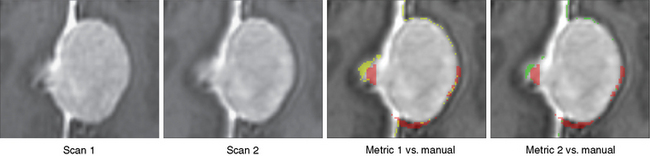
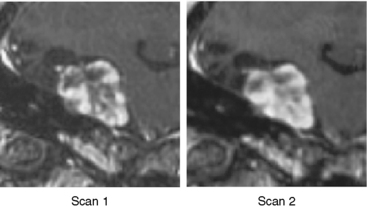
We then repeated the tumor growth analysis with our semi-automatic tool. Figure 17-3 shows an example of the analysis in which yellow corresponds to the first automatic metric, green corresponds to the second automatic metric, and red corresponds to the manual results. In seven out of the nine cases, the variations between automatic and manual measurements were within the expected range of variations found across experts’ segmentations. Further, the follow-up study by Konukoglu and colleagues¹⁹ showed that our automatic measure was more consistent in detecting subtle growth compared to manual measures. Figure 17-4 shows one of the two cases where our method disagreed with the manual findings. The intensity patterns of the tumor vary considerably between the acquisitions, which is unusual in our experience, and violates one of the underlying assumptions of the pipeline. The inconsistencies observed in the second case were due to the tumor’s relatively small size (334 mm³). In this case, distinguishing growth from interpolation artifacts is relatively difficult. However, not all radiologists we consulted diagnosed these two cases as meningiomas.

FIGURE 17-4 Our approach had difficulties analyzing growth due to uncommon changes in the intensity profile between the two scans, as shown in the images to the left.

CONCLUSION

We have discussed an approach that successfully measures the volume change of slowly evolving meningiomas from successive MRI scans. The correlation to expert findings shows the potential for the software tool to be used in standard clinical practice. The experiment not only reveals the need for observer-independent tools for detecting volume change in slowly growing tumors but also provides a possible solution.