Assessment of biopharmaceutical properties
Marianne Ashford
Chapter contents
Measurement of key biopharmaceutical properties
Release of drug from its dosage form into solution
Stability in physiological fluids
Plasma concentration-time curves
Cumulative urinary drug excretion curves
Absolute and relative bioavailability
Assessment of site of release in vivo
Key points
Introduction
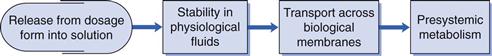
Biopharmaceutics is concerned with factors that influence the rate and extent of drug absorption. As discussed in Chapters 19 and 20, the factors that affect the release of a drug from its dosage form, its dissolution into physiological fluids, its stability within those fluids, its permeability across the relevant biological membranes and its presystemic metabolism will all influence its rate and extent of absorption (Fig. 21.1). Once the drug is absorbed into the systemic circulation, its distribution within the body tissues (including to its site of action), its metabolism and elimination are described by the pharmacokinetics of the compound (discussed in Chapter 18). This in turn influences the length and magnitude of the therapeutic effect or the response of the compound, i.e. its pharmacodynamics.
The key biopharmaceutical properties that can be quantified and therefore give an insight into the absorption of a drug are its:
• release from its dosage form into solution at the absorption site
As most drugs are delivered via the mouth, these properties will be discussed with respect to the peroral route. The bioavailability of a compound is an overall measure of its availability in the systemic circulation and so the assessment of bioavailability will also be discussed. Other methods of assessing the performance of dosage forms in vivo will also be briefly mentioned. The Biopharmaceutics Classification System (BCS), which classifies drugs according to dose and two of their key biopharmaceutical properties, solubility and permeability, is outlined.
Measurement of key biopharmaceutical properties
Release of drug from its dosage form into solution
As discussed in Chapter 20 and Part 5 of this book, a dosage form is normally formulated to aid and/or control the release of drug from it. For example, for an immediate-release tablet, the tablet needs to disintegrate to yield the primary drug particles. Further, a suspension should not be so viscous that it impedes the diffusion of dissolving drug away from the solid particles.
The solubility of a drug across the gastrointestinal pH range will be one of the first indicators as to whether dissolution is liable to be rate limiting in the absorption process. Knowledge of the solubility across the gastrointestinal pH range can be determined by measuring the equilibrium solubility in suitable buffers or by using an acid or a base titration method.
Methods of measuring the dissolution rate of both a drug itself (intrinsic dissolution rate) and of various dosage forms are discussed in Chapters 2 and 35, and in the relevant chapters of Part 5.
The aim of dissolution testing is to find an in vitro characteristic of a potential formulation that reflects its in vivo performance. When designing a dissolution test to assess drug release from a biopharmaceutical perspective, it is important to mimic as closely as possible the conditions of the gastrointestinal tract. Clinical scientists increasingly want to rely on dissolution tests to establish in vitro/in vivo correlations between the release of drug from the dosage form and its absorption. If this can be successfully achieved, it is possible that the dissolution test could replace some of the in vivo studies that need to be performed during product development and registration. Such correlations should have the benefits of reducing the use of animals to evaluate formulations and the size and number of costly clinical studies to assess bioavailability as well as being used to allow formulation, process and site of manufacture changes.
An in-vitro/in-vivo correlation may only be possible for those drugs where dissolution is the rate-limiting step in the absorption process. Determining full dissolution profiles of such drugs in a number of different physiologically representative media will aid the understanding of the factors affecting the rate and extent of dissolution. The profiles can also be used to generate an in vitro/in vivo correlation. To achieve this, at least three batches that differ in their in vivo as well as their in vitro behaviour should be available. The differences in the in vivo profiles need to be mirrored by the formulations in vitro. Normally, the in vitro test conditions can be modified to correspond with the in vivo data to achieve a correlation. Very often, a well-designed in vitro dissolution test is found to be more sensitive and discriminating than an in vivo test. From a quality assurance perspective, a more discriminating dissolution method is preferred because the test will indicate possible changes in the product before the in vivo performance is affected.
In-vitro dissolution testing of solid dosage forms is discussed fully in Chapter 35. The reader is referred there for consideration of the apparatus available and suitable dissolution media to simulate as closely as possible gastric and intestinal fluids. This application of dissolution testing is discussed further here in the context of the assessment of biopharmaceutical properties.
A dilute hydrochloric acid-based solution at pH 1.2 can simulate gastric fluid quite closely (but obviously not exactly) and phosphate-buffered solution at pH 6.8 can mimic intestinal fluid. However, dissolution media more closely representing physiological conditions may well provide more relevant conditions. A range of dissolution media that are widely accepted to mimic physiological parameters in gastric and intestinal fluids in the fed and fasted states are available. Each of these media takes into account not only the pH of the fluids in the different states but their ionic composition, surface tension, buffer capacity and bile and lecithin contents. Details of simulated gastric and intestinal fluids for both the fed and fasted state are given in Tables 35.2 and 35.3.
The conditions within the stomach in the fed state are highly dependent on the composition of the meal eaten and are therefore difficult to simulate. In trying to produce an in vitro/in vivo correlation, it has been suggested that a more appropriate way of simulating the fed-state gastric fluids is to homogenize the meal to be used in clinical studies and then dilute it with water. Long-life milk has also been used to simulate gastric conditions in the fed state.
It has been proposed that the duration of the dissolution test should depend on the site of absorption of the drug and its timing of administration. Thus, in designing a dissolution test, some knowledge or prediction of the permeability properties of the drug is beneficial. If, for example, the drug is absorbed from the upper intestine and is likely to be dosed in the fasted state, the most appropriate dissolution conditions may be a short test (~5–30 minutes) in a medium simulating gastric fluid in the fasted state. Alternatively, if it is advised that a drug should be administered with food and the drug is known to be well absorbed throughout the length of the gastrointestinal tract, a far longer dissolution test may be more appropriate. This could perhaps be several hours in duration with a range of media such as, initially, simulated gastric fluid to mimic the fed state, followed by simulated intestinal fluid to mimic both fed and fasted states.
The volumes of fluid within, and the degree of agitation of, the stomach and intestines vary enormously, particularly between the fed and the fasted states. Consequently, it is difficult to choose a representative volume and degree of agitation for an in vitro test. Guidance given to industry on the dissolution testing of immediate-release solid oral dosage forms suggests volumes of 500, 900 or 1000 mL and gentle agitation conditions. Regulatory authorities will expect justification of a dissolution test to ensure that it will discriminate between a good and a poor formulation, and thus see it as a critical quality test in submissions of applications for Marketing Authorizations.
Stability in physiological fluids
The stability of drugs in physiological fluids (in the case of orally administered drugs, the gastrointestinal fluids) depends on two factors:
Means of assessing the chemical stability of a drug are discussed in Chapters 48 and 49. The stability of a drug in gastrointestinal fluids can be assessed by simulated gastric and intestinal media or by obtaining gastrointestinal fluids from humans or animals. The latter provides a harsher assessment of gastrointestinal stability but is more akin to the in vivo setting. In general, the drug is incubated with either real or simulated fluid at 37 °C for a period of 3 hours and the drug content analysed. A loss of more than 5% of drug indicates potential instability. Many of the permeability methods described below can be used to identify whether gastrointestinal stability is an issue for a particular drug.
For drugs that will still be in the gastrointestinal lumen when they reach the colonic region, resistance to the bacterial enzymes present in this part of the intestine needs to be considered. The bacterial enzymes are capable of a whole host of reactions. There may be a significant portion of a poorly soluble drug still in the gastrointestinal tract by the time it reaches the colon. If the drug is absorbed along the length of the gastrointestinal tract, and is susceptible to degradation or metabolism by the bacterial enzymes within the tract, the drug’s absorption and hence its bioavailability is liable to be reduced. Similarly, for sustained- or controlled-release products that are designed to release their drug along the length of the gastrointestinal tract, the potential of degradation or metabolism by bacterial enzymes should be assessed. If a drug is metabolized to a metabolite which can be absorbed, the potential toxicity of this metabolite should be considered.
Permeability
There is a wealth of techniques available for either estimating or measuring the rate of permeation across membranes that are used to gain an assessment of oral absorption in humans. These range from computational (in silico) predictions to both physicochemical and biological methods. The biological methods can be further subdivided into in vitro, in situ and in vivo methods. In general, the more complex the technique, the more information that can be gained and the more accurate is the assessment of oral absorption in humans. The range of techniques is summarized in Table 21.1. Some of the more widely used ones are discussed below.
Table 21.1
Some of the models available for predicting or measuring drug absorption
| Model type | Model | Description |
| Computational/In silico | clog P | Commercial software that calculates n-octanol/ water partition coefficient based on fragment analysis, known as the Leo-Hansch method |
| mlog P | Method of calculating log P, known as the Moriguchi method (see text) | |
| Physicochemical | Partition coefficient | Measure of lipophilicity of drug, usually measured between n-octanol and aqueous buffer via a shake-flask method |
| Immobilized artificial membrane | Measures partition into more sophisticated lipidic phase on an HPLC column | |
| Cell culture | Caco-2 monolayer | Measures transport across monolayers of differentiated human colon adenocarcinoma cells |
| HT-29 | Measures transport across polarized cell monolayer with mucin-producing cells | |
| Excised tissues | Cells | Measures uptake into cell suspensions, e.g. erythrocytes |
| Freshly isolated cells | Measures uptake into enterocytes; however; the cells are difficult to prepare and are short-lived | |
| Membrane vesicles | Measures uptake into brush border membrane vesicles prepared from intestinal scrapings or isolated enterocytes | |
| Everted sacs | Measures uptake into intestinal segments/sacs | |
| Everted intestinal rings | Studies the kinetics of uptake into the intestinal mucosa | |
| Isolated sheets | Measures the transport across sheets of intestine | |
| In situ studies | In situ perfusion | Measures drug disappearance from either closed or open loop perfusate of segments of intestine of anaesthetized animals |
| Vascularly perfused intestine | Measures drug disappearance from perfusate and its appearance in blood | |
| In vivo studies | Intestinal loop | Measures drug disappearance from perfusate of loop of intestine in awake animal |
| Human data | Loc-I-Gut | Measures drug disappearance from perfusate of human intestine |
| High-frequency capsule | Non-invasive method; measures drug in systemic circulation | |
| InteliSite capsule | Non-invasive method; measures drug in systemic circulation | |
| Bioavailability | Deconvolution of pharmacokinetic data |
Partition coefficients
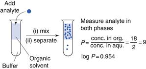
One of the first properties of a molecule that should be predicted or measured is its partition coefficient between oil and a water phase (log P). This gives a measure of the lipophilicity of a molecule, which can be used to predict how well it will be able to cross a biological membrane. It is a very useful parameter for many reasons relating to formulation design and drug absorption and is discussed elsewhere in Chapters 2, 20 and 23. As discussed in Chapter 20, n-octanol is most commonly chosen as the solvent for the oil phase as it has similar properties to biological membranes although other oil phases have been used (as considered in Chapter 23). One of the most common ways of measuring partition coefficients is to use the shake flask method (Fig. 21.2). It relies on the equilibrium distribution of a drug between oil and an aqueous phase. Prior to the experiment the aqueous phase should be saturated with the oil phase and vice versa. The experiment should be carried out at constant temperature. The drug should be added to the aqueous phase and the oil phase which, in the case of n-octanol, as it is less dense than water, will sit on top of the water. The system is mixed and then left to reach equilibrium (usually at least 24 hours). The two phases are separated and the concentration of drug is measured in each phase and a partition coefficient calculated. This technique is discussed further in the context of preformulation in Chapter 23.
If the aqueous phase is at a particular pH, the distribution coefficient at that pH is measured (log D); this then accounts for the ionization of the molecule at that pH. In the case of a weakly acidic or a weakly basic drug, the log D measured at an intestinal pH (e.g. 6.8) is liable to give a better prediction of the drug’s ability to cross the lipid gastrointestinal membrane than its partition coefficient, log P, which does not take the degree of ionization into account.
As discussed in Chapter 20, within a homologous series, increasing lipophilicity (log P or log D) tends to result in greater absorption. A molecule is unlikely to cross a membrane (i.e. be absorbed via the transcellular passive route) if it has a log P less than 0.
Instead of determining log P experimentally, computational methods can be used to estimate it. There are a number of software packages available to do this. There is a reasonably good correlation between calculated and measured values. Log P can be estimated by breaking down the molecule into fragments and calculating the contribution of each fragment to overall lipophilicity (often called the clog P). Another way of estimating log P is the Moriguchi method, which uses 13 parameters for hydrophobic and hydrophilic atoms, proximity effects, unsaturated bonds, intramolecular bonds, ring structures, amphoteric properties and several specific functionalities to obtain a value for the partition coefficient. This is often called the mlog P. The advantages of these methods are in drug discovery, where an estimate of the lipophilicity of many molecules can be obtained before they are actually synthesized.
Another, more sophisticated physicochemical means of estimating how well a drug will partition into a lipophilic phase is by investigating how well the molecule can be retained on a high-performance liquid chromatography (HPLC) column. HPLC columns can be simply coated with n-octanol to mimic n-octanol-aqueous partition or, more elaborately, designed to mimic biological membranes. For example the immobilized artificial membrane (IAM) technique provides a measure of how well a solute (i.e. the drug) in the aqueous phase will partition into biological membranes (i.e. be retained on the column). Good correlations between these methods and biological in vitro methods of estimating transcellular passive drug absorption have been obtained.
Cell culture techniques
Cell culture techniques for measuring the intestinal absorption of molecules have been increasingly used over recent decades and are now a well-accepted model for absorption. The cell line that is most widely used is Caco-2.
Caco-2 cells are a human colon carcinoma cell line that was first-proposed and characterized as a model for oral drug absorption by Hidalgo. In culture, Caco-2 cells spontaneously differentiate to form a monolayer of polarized enterocytes. These enterocytes resemble those in the small intestine, in that they possess microvilli and many of the transporter systems present in the small intestine, for example those for sugars, amino acids, peptides and the P-glycoprotein efflux transporter. Adjacent Caco-2 cells adhere through tight junctions. However, the tightness of these junctions is more like those of the colon than those of the leakier small intestine.
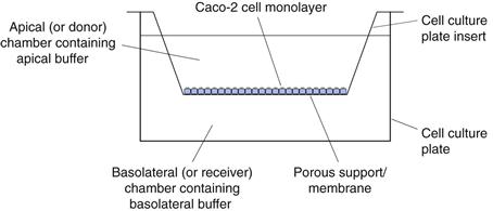
There are many variations on growing and carrying out transport experiments with Caco-2 monolayers. In general, the cells are grown on porous supports, usually for a period of 15–21 days in typical cell culture medium, Dulbecco’s Modified Eagle Medium supplemented with 20% foetal bovine serum, 1% non-essential amino acids and 2 mM L-glutamine. The cells are grown at 37 °C in 10% carbon dioxide at a relative humidity of 95%. The culture medium is replaced at least twice each week. Transport experiments are carried out by replacing the culture medium with buffers, usually Hank’s Balanced Salt Solution adjusted to pH 6.5 on the apical surface and Hank’s Balanced Salt Solution adjusted to pH 7.4 on the basolateral surface (Fig. 21.3).
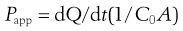
After a short incubation period, usually about 30 minutes, when the cells are maintained at 37°C in a shaking water bath, the buffers are replaced with fresh buffers and a dilute solution of drug is introduced to the apical chamber. At regular intervals, the concentration of the drug in the basolateral chamber is determined. The apparent permeability coefficient across cells can be calculated as follows:
 (21.1)
where Papp is the apparent permeability coefficient (cm/s), dQ/dt is the rate of drug transport (µg s−1), C0 is the initial donor concentration (mg/mL) and A is the surface area of the monolayer (cm2).
To check that the monolayer has maintained its integrity throughout the transport process, a marker for paracellular absorption, such as mannitol, which is often radiolabelled for ease of assay, is added to the apical surface. If less than 2% of this crosses the monolayer in an hour then the integrity of the monolayer has been maintained. Another way to check the integrity of the mono-layer is by measuring the transepithelial resistance (TER).
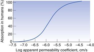
To use the Caco-2 cells as an absorption model, a calibration curve needs to be generated. This is done for compounds for which the absorption in humans is known. Figure 21.4 shows the general shape of the curve of fraction absorbed in humans versus the apparent permeability coefficient in Caco-2 cells. As cells are biological systems, small changes in their source, method of culture and the way in which the transport experiment is performed will affect the apparent permeability of a drug, such that this curve can shift significantly to the right or left, or alter in its gradient. Therefore, when carrying out Caco-2 experiments, it is important always to standardize the procedure within a particular laboratory and ensure that this procedure is regularly calibrated with a set of standard compounds.
Caco-2 monolayers can also be used to elucidate the mechanism of permeability. If the apparent permeability coefficient is found to increase linearly with increasing concentration of drug (i.e. the transport is not saturated), is the same whether the drug transport is measured from the apical to basolateral or the basolateral to apical direction, and is independent of pH, it can be concluded that the transport is a passive and not an active process. If the transport in the basolateral to apical direction is significantly greater than that in the apical to basolateral direction then it is likely that the drug is actively effluxed from the cells by a counter-membrane transporter, such as P-glycoprotein. If the transport of the drug is also inhibited by the presence of compounds that are known inhibitors of P-glycoprotein this gives a further indication that the drug is susceptible to P-glycoprotein efflux.
To help elucidate whether other membrane transporters are involved in the absorption of a particular drug, further competitive inhibition studies can be carried out with known inhibitors of the particular transporter. For example, the dipeptide glycosyl-sarcosine can be used to probe whether the dipeptide transporter is involved in the absorption of a particular drug.
To evaluate whether a compound is absorbed via the paracellular or the transcellular pathway, the tight junctions can be artificially opened with compounds such as EDTA, which chelates calcium. Calcium is involved in keeping the junctions together. If the apparent permeability of a compound is not affected by the opening of these junctions, which can be assessed by using a paracellular marker such as mannitol, one can assume the drug transport is via a transcellular pathway.
If the disappearance of drug on the apical side of the membrane is not mirrored by its appearance on the basolateral side, and/or the mass balance at the end of the transport experiment does not account for 100% of the drug, there may be a problem with binding to the membrane porous support. This will need investigation, or the drug may have a stability issue. The drug could be susceptible to enzymes secreted by the cells and/or to degradation by hydrolytic enzymes as it passes through the cells, or it may be susceptible to metabolism by cytochrome P450 within the cell. Thus the Caco-2 cells are not only capable of evaluating the permeability of drugs but also have value in investigating whether two of the other potential barriers to absorption, namely stability and presystemic metabolism, are likely to affect the overall rate and extent of absorption.
Caco-2 cells are very useful tools for understanding the mechanism of drug absorption and have furthered significantly our knowledge of the absorption of a variety of drugs. Other advantages of Caco-2 cells are that they are a non-animal model, require only small amounts of compound for transport studies, can be used as a rapid screening tool to assess the permeability of large numbers of compounds in the discovery setting and can be used to evaluate the potential toxicity of compounds to cells. The main disadvantages of Caco-2 monolayers as an absorption model are that, because of the tightness of the monolayer, they are more akin to the paracellular permeability of the colon rather than that of the small intestine and that they lack a mucus layer.
Further information on the use of Caco-2 monolayers as an absorption model can be obtained from Artusson et al (1996) and Yang and Yu (2009).
Tissue techniques
A range of tissue techniques have been used as absorption models (Table 21.1). Two of the more popular ones are the use of isolated sheets of intestinal mucosa and of everted intestinal rings. These are discussed in more detail below.
Isolated sheets of intestinal mucosa are prepared by cutting the intestine into strips. The musculature is then removed and the sheet mounted and clamped in a diffusion chamber or an Ussing chamber filled with appropriate biological buffers (Fig. 21.5). The transepithelial resistance is measured across the tissue to check its integrity. The system is maintained at 37 °C and stirred so that the thickness of the unstirred water layer is controlled and oxygen provided to the tissue. The drug is added to the donor chamber and the amount accumulating in the receiver chamber is measured as a function of time. The permeability across the tissue can then be calculated.
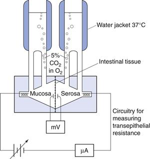
Fig. 21.5 Diagram of a diffusion chamber.
Similar to cell monolayers, the two sides of the tissue can be sampled independently and thus fluxes from mucosal to serosal and from serosal to mucosal sides can be measured. Any pH dependence of transport can be determined by altering the pH of the buffers in the donor and/or receiver chambers. This system can also therefore be used to probe active transport.
One advantage of this technique over cell culture techniques is that permeability across different regions of the intestine can be assessed. It is particularly helpful to be able to compare permeabilities across intestinal and colonic tissue, especially when assessing whether a drug is suitable for a controlled-release delivery system. In addition, different animal tissues that permit an assessment of permeability in different preclinical models can be used. The rat intestine is usually preferred for absorption studies as its permeability correlates well with that of human intestine. Human tissue and cell monolayers have also been used in this system.
Everted intestinal rings use whole intestinal segments rather than just sheets. The musculature is therefore intact. Intestinal segments are excised, again usually from rats. The segment is then tied at one end and carefully everted by placing it over a glass rod. It is cut into small sections or rings and these rings incubated in stirred oxygenated drug-containing buffer at 37 °C. After a set period of time, drug uptake is quenched by quickly rinsing the ring with ice-cold buffer and carefully drying it. The ring is then assayed for drug content and the amount of drug taken up per gram of wet tissue over a specific period of time is calculated (mol g−1 time−1). The advantage of using intestinal rings is that the test is relatively simple and quick to perform. A large number of rings can be prepared from each segment of intestine, which allows each animal to act as its own control. In addition, the conditions of the experiment can be manipulated and so provide an insight into the mechanisms of absorption.
The disadvantages of this system are that it is biological and that care must be taken to maintain the viability of the tissue for the duration of the experiment. As the drug is taken up into the ring, the tissue needs to be digested and the drug extracted from it before it is assayed. This results in lengthy sample preparation and complicates the assay procedure. In addition, as this is an uptake method, no polarity of absorption can be assessed.
Both these absorption models can be calibrated with a standard set of compounds similar to the Caco-2 model. A similarly shaped curve for the percentage of drug absorbed in humans versus apparent permeability or uptake (mole per weight of tissue) for the isolated sheet and everted ring methods, respectively, is obtained.
Perfusion studies
Many variations of intestinal perfusion methods have been used as absorption models over the years. In general, because of its relative ease of use and similarity to the permeability of the human intestine, the rat model is preferred. In situ intestinal perfusion models have the advantage that the whole animal is used, with the nerve, lymphatic and blood supplies intact. Therefore there should be no problem with tissue viability and all the transport mechanisms present in a live animal should be functional.
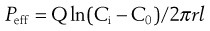
The animal is anaesthetized and the intestine exposed. In the open loop method a dilute solution of drug is pumped slowly through the intestine and the difference in drug concentration between the inlet and outlet concentrations is measured (Fig. 21.6). An absorption rate constant or effective permeability coefficient across the intestine can be calculated as follows:
 (21.2)
where Peff is the effective permeability coefficient (cm/s), Q is the flow rate in mL s−1, Ci is the initial drug concentration, C0 is the final drug concentration, r is the radius of the intestinal loop (cm), and, l is the length of intestinal loop (cm).
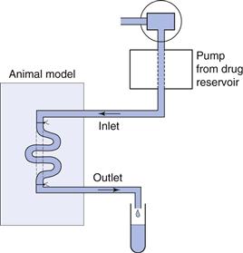
Fig. 21.6 Diagram of an in situ rat perfusion.
In the closed loop method a dilute solution of drug is added to a section of the intestine and the intestine closed. The intestine is then excised and drug content analysed immediately and after an appropriate time or time intervals, depending on the expected rate of absorption. Again, assuming a first-order rate process and hence an exponential loss of drug from the intestine, an absorption rate constant and effective permeability can be calculated. Like the intestinal ring method, the closed loop in situ perfusion model requires a lengthy digestion, extraction and assay procedure to analyse the drug remaining in the intestinal loop.
There is a lot of fluid moving in and out of the intestine and so the drug concentrations in both these in situ perfusion methods need to be corrected for fluid flux. This is normally done by gravimetric means or by using a non-absorbable marker to assess the effect of fluid flux on the drug concentration. As with other absorption models, correlations have been made with standard compounds where the fraction absorbed in humans is known (see Fig. 21.4). In these models the ‘absorption rate’ is calculated by measuring the disappearance of the drug from the lumen and not its accumulation in the plasma. It is therefore important to check that the drug is not degraded in the lumen or intestinal wall as drug that has disappeared will be erroneously assumed to have been absorbed.
More sophisticated techniques are those involving vascular perfusion. In these techniques, either a pair of mesenteric vessels supplying an intestinal segment or the superior mesenteric artery and portal vein perfusing almost the entire intestine are cannulated. The intestinal lumen and sometimes the lymph duct are also cannulated for the collection of luminal fluid and lymph, respectively. This model, although complicated, is very versatile as drug can be administered into the luminal or the vascular perfusate. When administered to the intestinal lumen, drug absorption can be evaluated from both its disappearance from the lumen and its appearance in the portal vein. Using this method, both the rate and extent of absorption can be estimated, as well as carrier-mediated transport processes. Collection of the lymph allows the contribution of lymphatic absorption for very lipophilic compounds to be assessed. One of the other advantages of this system is the ability to determine whether any intestinal metabolism occurs before or after absorption.
A further extension of this model is to follow the passage of drugs from the intestine through the liver, and several adaptations of rat intestinal-liver perfusion systems have been investigated. Such a combined system gives the added advantage of assessing the first-pass or presystemic metabolism through the liver, and determining the relative importance of the intestine and liver in presystemic metabolism.
The disadvantage of these perfusion systems is that as they become more complex, a larger number of animals are required to establish suitable perfusion conditions and the reproducibility of the technique. However, in general, as the complexity increases so does the amount of information obtained.
Assessment of permeability in humans
Intestinal perfusion studies.
Until relatively recently, the most common way to evaluate the absorption of drugs in humans was by performing bioavailability studies and deconvoluting the data available to calculate an absorption rate constant. This rate constant, however, is dependent on the release of the drug from the dosage form and is affected by intestinal transit and presystemic metabolism. Therefore, very often it does not reflect the true intrinsic intestinal permeability of a drug.
Extensive studies have been carried out using a regional perfusion technique which has afforded a greater insight into human permeability (Loc-I-Gut). The Loc-I-Gut is a multichannel tube system with a proximal and a distal balloon (Fig. 21.7). These balloons are 100 mm apart and allow a segment of intestine 100 mm long to be isolated and perfused. Once the proximal balloon passes the ligament of Treitz, both balloons are filled with air, thereby preventing mixing of the luminal contents in the segment of interest with other luminal contents. A non-absorbable marker is used in the perfusion solution to check that the balloons work to occlude the region of interest. A tungsten weight is placed in front of the distal balloon to facilitate its passage down the gastrointestinal tract.
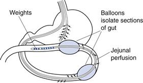
Fig. 21.7 Diagram of the Loc-I-Gut.
Drug absorption is calculated from the rate of disappearance of the drug from the perfused segment. This technique has afforded greater control in human intestinal perfusions, primarily because it isolates the luminal contents of interest, and has greatly facilitated the study of permeability mechanisms and the metabolism of drugs and nutrients in the human intestine.
Non-invasive approaches.
There is concern that the invasive nature of perfusion techniques can affect the function of the gastrointestinal tract, in particular the fluid content, owing to the intubation process altering the absorption and secretion balance. To overcome this problem, several engineering-based approaches have been developed to evaluate drug absorption in the gastrointestinal tract. These include the InteliSite® and the Enterion®capsules and the MAARS® capsule.
The InteliSite capsule is a radiofrequency-activated, non-disintegrating delivery device. Either a liquid or a powder formulation can be filled into the capsule, the transit of which is followed by γ-scintigraphy (see later in this chapter). Once the capsule reaches its desired release site, it is externally activated to open a series of windows to the drug reservoir within the capsule. The Enterion capsule is similar in that it contains a drug reservoir and uses γ-scinitigraphy to locate the capsule in the gastrointestinal tract. However, its payload is released via an electromagnetic field triggering the actuation of a spring resulting in the instantaneous release of the formulation as a bolus. For both these systems, blood samples need to be taken to quantify drug absorption. The MAARS® system is a magnetic active agent release system and thus relies on a magnetic impulse to disassemble the capsule and release the drug; this is a simpler system and can contain a large volume of drug. More sophisticated systems with cameras incorporated into capsules, such as the M2A capsule, are being developed to visualize the gastrointestinal tract. These can be used to help design better products.
Presystemic metabolism
Presystemic metabolism is the metabolism that occurs before the drug reaches the systemic circulation. Therefore, for an orally administered drug, this includes the metabolism that occurs in the gut wall and the liver. As discussed above, perfusion models that involve both the intestines and the liver allow an evaluation of the presystemic metabolism in both organs. In other models it is sometimes possible to design mass balance experiments that will assess whether presystemic intestinal metabolism is likely to occur.
Intestinal cell fractions, such as brush border membrane preparations that contain an abundance of hydrolytic enzymes, and homogenized preparations of segments of rat intestine can also be used to determine intestinal presystemic metabolism. Drugs are incubated with either brush border membrane preparations or gut wall homogenate at 37 °C and the drug content analysed.
Various liver preparations, for example subcellular fractions such as microsomes, isolated hepatocytes and liver slices, are used to determine hepatic metabolism in vitro. These are classified as phase I metabolism, which mainly involves oxidation but can be reduction or hydrolysis, and phase II metabolism, which follows phase I and involves conjugation reactions. Microsomes are prepared by high-speed centrifugation of liver homogenates (100 000 g) and are composed mainly of fragments of the endoplasmic reticulum. They lack cystolic enzymes and cofactors and are therefore only suitable to evaluate some of the metabolic processes (phase I metabolism) of which the liver is capable. Hepatocytes must be freshly and carefully prepared from livers and are only viable for a few hours. It is therefore difficult to obtain human hepatocytes. Hepatocytes are very useful for hepatic metabolism studies as it is possible to evaluate most of the metabolic reactions, i.e. both phase I and II metabolism. Whole liver slices again have the ability to evaluate both phase I and II metabolism. As liver slices are tissue slices rather than cell suspensions, and because they do not require enzymatic treatment in their preparation, they may give a higher degree of in vivo correlation than hepatocytes or microsomes.
Assessment of bioavailability
The measurement of bioavailability gives the net result of the effect of the release of drug into solution in the physiological fluids at the site of absorption, its stability in those physiological fluids, its permeability and its presystemic metabolism on the rate and extent of drug absorption by following the concentration-time profile of drug in a suitable physiological fluid. The concentration-time profile also gives information on other pharmacokinetic parameters, such as the distribution and elimination of the drug. The most commonly used method of assessing the bioavailability of a drug involves the construction of a blood plasma concentration-time curve, but urine drug concentrations can also be used and are discussed below.
Plasma concentration-time curves
When a single dose of a drug is administered orally to a patient, serial blood samples are withdrawn and the plasma assayed for drug concentration at specific time points after administration. This enables a plasma concentration-time curve to be constructed. Figure 21.8 shows a typical plasma concentration-time curve following the oral administration of a tablet.
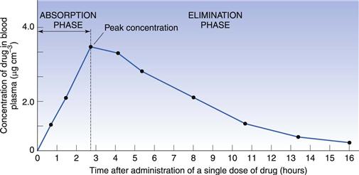
At zero time, when the drug is first administered, the concentration of drug in the plasma will be zero. As the tablet passes into the stomach and/or intestine it disintegrates, the drug dissolves and absorption occurs. Initially, the concentration of drug in the plasma rises as the rate of absorption exceeds the rate at which the drug is being removed by distribution and elimination. Concentrations continue to rise until a maximum (or peak) is attained. This represents the highest concentration of drug achieved following the administration of a single dose, often termed the Cmax (or Cpmax in the specific case of maximum plasma concentration). It is reached when the rate of appearance of drug in the plasma is equal to its rate of removal by distribution and elimination.
The ascending portion of the plasma concentration-time curve is sometimes called the absorption phase. Here the rate of absorption outweighs the rate of removal of drug by distribution and elimination. Drug absorption does not usually stop abruptly at the time of peak concentration but may continue for some time into the descending portion of the curve. The early descending portion of the curve can thus reflect the net result of drug absorption, distribution, metabolism and elimination. In this phase, the rate of drug removal from the blood exceeds the absorption rate and therefore the concentration of the drug in the plasma declines.
Eventually drug absorption ceases when the bioavailable dose has been absorbed, and the concentration of drug in the plasma is now controlled only by its rate of elimination by metabolism and/or excretion. This is sometimes called the elimination phase of the curve. It should be appreciated, however, that elimination of a drug begins as soon as it appears in the plasma.
Several parameters based on the plasma concentration-time curve that are important in bioavailability studies are shown in Figure 21.9, and are discussed below.
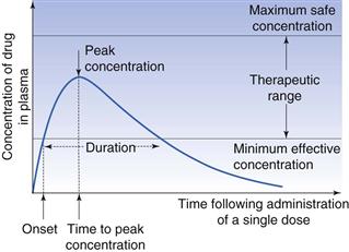
Minimum effective (or therapeutic) plasma concentration.
It is generally assumed that some minimum concentration of drug in the plasma must be reached before the desired therapeutic or pharmacological effect is achieved. This is called the minimum effective (or minimum therapeutic) plasma concentration. Its value not only varies from drug to drug but also from individual to individual and with the type and severity of the disease state. In Figure 21.9 the minimum effective concentration is indicated by the lower line.
Maximum safe concentration.
The concentration of drug in the plasma above which side-effects or toxic effects occur is known as the maximum safe concentration.
Therapeutic range or window.
A range of plasma drug concentrations is also assumed to exist over which the desired response is obtained, yet toxic effects are avoided. This range is called the therapeutic range or therapeutic window. The intention in clinical practice is to maintain plasma drug concentrations within this range.
Onset.
The onset may be defined as the time required to achieve the minimum effective plasma concentration following administration of the dosage form.
Duration.
The duration of the therapeutic effect of the drug is the period during which the concentration of drug in the plasma exceeds the minimum effective plasma concentration.
Peak concentration.
The peak concentration represents the highest concentration of the drug achieved in the plasma, often referred to as the Cmax.
Time to peak concentration.
This is the period of time required to achieve the peak plasma concentration of drug after the administration of a single dose. This parameter is related to the rate of absorption of the drug and can be used to assess that rate. It is often referred to as the Tmax.
Area under the plasma concentration-time curve.
This is related to the total amount of drug absorbed into the systemic circulation following the administration of a single dose, and is often known as the AUC.
Use of plasma concentration-time curves in bioavailability studies
In order to illustrate the usefulness of plasma concentration-time curves in bioavailability studies in the assessment of the rate and extent of absorption, the administration of single equal doses of three different formulations, A, B and C of the same drug to the same healthy individual by the same route of administration on three separate occasions can be considered. The assumption is made that sufficient time is allowed to elapse between the administration of each formulation such that the systemic circulation contained no residual concentration of drug and no residual effects from any previous administrations. It is also assumed that the kinetics and pattern of distribution of the drug, its binding phenomena, the kinetics of elimination and the experimental conditions under which each plasma concentration-time profile is obtained are the same on each occasion. The plasma concentration-time profiles for the three formulations are shown in Figure 21.10. The differences between the three curves are attributed solely to differences in the rate and/or extent of absorption of the drug from each formulation.
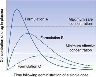
The three plasma profiles in Figure 21.10 show that each of the three formulations (A, B and C) of the same dose of the same drug results in different peak plasma concentrations. The area under the curves for formulations A and B are similar indicating that the drug is absorbed to a similar extent from these two formulations. However, the absorption rate is different with the drug being absorbed faster from formulation A than from formulation B. This means that formulation A shows a fast onset of therapeutic action but as its peak plasma concentration exceeds the maximum safe concentration, it is likely that this formulation will result in toxic side-effects. Formulation B, which has a slower rate of absorption than A, shows a slower therapeutic onset than A, but its peak plasma concentration lies within the therapeutic range. In addition, the duration of action of the therapeutic effect obtained with formulation B is longer than that obtained with A. Hence formulation B appears to be superior to formulation A from a clinical viewpoint, in that its peak plasma concentration lies within the therapeutic range of the drug and the duration of the therapeutic effect is longer.
Formulation C gives a much smaller area under the plasma concentration-time curve, indicating that a lower proportion of the dose has been absorbed. This, together with the slower rate of absorption from formulation C (the time of peak concentration is longer than for formulations A and B), results in the peak plasma concentration not reaching the minimum effective concentration. Thus formulation C does not produce a therapeutic effect and consequently is clinically ineffective as a single dose.
This simple hypothetical example illustrates how differences in bioavailability exhibited by a given drug from different formulations can result in a patient being either over-, under- or correctly medicated.
It is important to realize that the study of bioavailability based on drug concentration measurements in the plasma (or urine or saliva) is complicated by the fact that such concentration-time curves are affected by factors other than the biopharmaceutical factors of the drug product itself. Factors such as:
• sex and age of the test subjects
• genetic differences in drug metabolism
• concomitant administration of other drugs
• stress
are some of the variables that can complicate the interpretation of bioavailability studies. As far as possible, studies should be designed to control these factors.
Although plots such as those in Figure 21.10 can be used to compare the relative bioavailability of a given drug from different formulations, they cannot be used indiscriminately to compare different drugs. It is quite usual for different drugs to exhibit different rates of absorption, metabolism, excretion and distribution, different distribution patterns and differences in their plasma binding phenomena. All of these will influence the plasma concentration-time curve. Therefore, it would be extremely difficult to attribute differences in the concentration-time curves obtained for different drugs presented in different formulations to differences in their bioavailabilities.
Cumulative urinary drug excretion curves
Measurement of the concentration of intact drug and/or its metabolite(s) in the urine can also be used to assess bioavailability.
When a suitable specific assay method is not available for the intact drug in the urine or the specific assay method available for the parent drug is not sufficiently sensitive, it may be necessary to assay the principal metabolite or intact drug plus its metabolite(s) in the urine to obtain an index of bioavailability. Measurements involving metabolite levels in the urine are only valid when the drug in question is not subject to metabolism prior to reaching the systemic circulation. If an orally administered drug is subject to intestinal metabolism or first-pass liver metabolism, then measurement of the principal metabolite or of intact drug plus metabolites in the urine would give an overestimate of the systemic availability of that drug. It should be remembered that the definition of bioavailability is in terms of the extent and the rate at which intact drug appears in the systemic circulation after the administration of a known dose.
The assessment of bioavailability by urinary excretion is based on the assumption that the appearance of the drug and/or its metabolites in the urine is a function of the rate and extent of absorption. This assumption is only valid when a drug and/or its metabolites are extensively excreted in the urine, and where the rate of urinary excretion is proportional to the concentration of the intact drug in the blood plasma. This proportionality does not hold if:
The important parameters in urinary excretion studies are the cumulative amount of intact drug and/or metabolites excreted and the rate at which this excretion takes place. A cumulative urinary excretion curve is obtained by collecting urine samples (resulting from the total emptying of the bladder) at known intervals after a single dose of the drug has been administered. Urine samples must be collected until all drug and/or its metabolites have been excreted (this is indicated by the cumulative urinary excretion curve becoming parallel to the abscissa) if a comparison of the extent of absorption of a given drug from different formulations or dosage forms is to be made. A typical cumulative urinary excretion curve and the corresponding plasma concentration-time curve obtained following the administration of a single dose of a given drug by the oral route to a subject is shown in Figure 21.11.
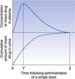
The initial segments (X-Y) of the curves reflect the absorption phase (i.e. where absorption is the dominant process) and the slope of this segment of the urinary excretion curve is related to the rate of absorption of the drug into the blood. The total amount of intact drug (and/or its metabolite(s) ) excreted in the urine at point Z corresponds to the time at which the plasma concentration of intact drug is zero and essentially all the drug has been eliminated from the body. The total amount of drug excreted at point Z may be quite different from the total amount of drug administered (i.e. the dose) either because of incomplete absorption or because of the drug being eliminated by processes other than urinary excretion.
Use of urinary drug excretion curves in bioavailability studies
In order to illustrate how cumulative urinary excretion curves can be used to compare the bioavailabilities of a given drug from different formulations, let us consider the urinary excretion data obtained following the administration of single equal doses of the three different formulations A, B and C of the same drug to the same healthy individual by the same extravascular route on three different occasions. Assume that these give the same plasma concentration-time curves as shown in Figure 21.10. The corresponding cumulative urinary excretion curves are shown in Figure 21.12.
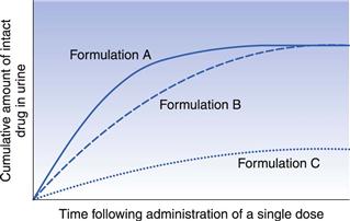
Fig. 21.12 Cumulative urinary excretion curves corresponding to the plasma concentration-time curves shown in Fig. 21.10 for three different formulations of the same drug administered in equal single doses by the same extravascular route.
The cumulative urinary excretion curves show that the rate at which drug appeared in the urine (i.e. the slope of the initial segment of each urinary excretion curve) from each formulation decreases in the order A > B > C. Because the slope of the initial segment of the urinary excretion curve is related to the rate of drug absorption, the cumulative urinary excretion curves indicate that the rates of absorption of drug from the three formulations decrease in the order A > B > C. The corresponding plasma concentration-time curves in Figure 21.10 shows that this is the case, i.e. peak concentration times (which are inversely related to the rate of drug absorption) for the three formulations increase in the order A > B > C. Although Figure 21.12 shows that the rate of appearance of drug in the urine from formulation A is faster than from B, the total amount of drug eventually excreted from these two formulations is the same, i.e. the cumulative urinary excretion curves for formulations A and B eventually meet and merge. As the total amount of intact drug excreted is assumed to be related to the total amount absorbed, the cumulative urinary excretion curves for formulations A and B indicate that the extent of drug absorption from these two formulations is the same. This is confirmed by the plasma concentration-time curves for formulations A and B in Figure 21.10 that exhibit similar areas under their curves.
Thus, both the plasma concentration-time curves and the corresponding cumulative urinary excretion curves for formulations A and B show that the extent of absorption from these formulations is equal, despite the drug being released at different rates from the respective formulations.
Consideration of the cumulative urinary excretion curve for C shows that this formulation not only results in a slower rate of appearance of intact drug in the urine but also that the total amount of drug eventually excreted is much less than from the other two formulations. This is confirmed by the plasma concentration-time curve shown in Figure 21.10 for formulation C.
Absolute and relative bioavailability
Absolute bioavailability
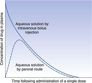
The absolute bioavailability of a given drug from a dosage form is the fraction (or percentage) of the administered dose which is absorbed intact into the systemic circulation. Absolute bioavailability may be calculated by comparing the total amount of intact drug that reaches the systemic circulation after the administration of a known dose of the dosage form via a route of administration, with the total amount that reaches the systemic circulation after the administration of an equivalent dose of the drug in the form of an intravenous bolus injection. An intravenous bolus injection is used as a reference to compare the systemic availability of the drug administered via different routes. This is because when a drug is delivered intravenously, the entire administered dose is introduced directly into the systemic circulation, i.e. it has no absorption barrier to cross, and is therefore considered to be totally bioavailable.
The absolute bioavailability of a given drug using plasma data may be calculated by comparing the total areas under the plasma concentration-time curves obtained following the administration of equivalent doses of the drug via any route of administration and that following delivery via the intravenous route in the same subject on different occasions. Typical plasma concentration-time curves obtained by administering equivalent doses of the same drug by the intravenous route (bolus injection) and the gastrointestinal route are shown in Figure 21.13.
For equivalent doses of administered drug:
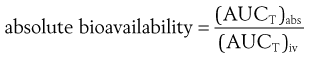 (21.3)
where (AUCT)abs is the total area under the plasma concentration-time curve following the administration of a single dose via an absorption site and (AUCT)iv is the total area under the plasma concentration-time curve following administration by rapid intravenous injection.
If different doses of the drug are administered by both routes, a correction for the sizes of the doses can be made as follows:
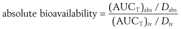 (21.4)
where Dabs is the size of the single dose of drug administered via the absorption site and Div is the size of the dose of the drug administered as an intravenous bolus injection. Sometimes it is necessary to use different dosages of drugs via different routes. Often the dose administered intravenously is lower to avoid toxic side-effects and for ease of formulation. Care should be taken when using different dosages to calculate bioavailability data as sometimes the pharmacokinetics of a drug are non-linear and different doses will then lead to an incorrect figure for the absolute bioavailability if calculated using a simple ratio, as in Equation 21.4.
Absolute bioavailability using urinary excretion data may be determined by comparing the total cumulative amounts of unchanged drug ultimately excreted in the urine following administration of the drug via an absorption site and the intravenous route (bolus injection) on different occasions to the same subject.
For equivalent doses of administered drug:
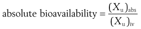 (21.5)
where (Xu)abs and (Xu)iv are the total cumulative amounts of unchanged drug ultimately excreted in the urine following administration of equivalent single doses of drug via an absorption site and as an intravenous bolus injection, respectively.
If different doses of drug are administered:
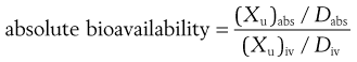 (21.6)
The absolute bioavailability of a given drug from a particular type of dosage form may be expressed as a fraction or, more commonly, as a percentage.
Measurements of absolute bioavailability obtained by administering a given drug in the form of a simple aqueous solution (that does not precipitate on contact with, or on dilution by, gastrointestinal fluids) by both the oral and the intravenous routes provide an insight into the effects that factors associated with the oral route may have on bioavailability, e.g. presystemic metabolism by the intestine or liver, the formation of complexes between the drug and endogenous substances (e.g. mucin) at the site of absorption and drug stability in the gastrointestinal fluids.
It should be noted that the value calculated for the absolute bioavailability will only be valid for the drug being examined if the kinetics of elimination and distribution are independent of the route and time of administration and the size of dose administered (if different doses are administered by the intravenous route and absorption site). If this is not the case, one cannot assume that the observed differences in the total areas under the plasma concentration-time curves or in the total cumulative amounts of unchanged drug ultimately excreted in the urine are due entirely to differences in bioavailability.
Relative bioavailability
In the case of drugs that cannot be administered by intravenous bolus injection, the relative (or comparative) bioavailability is determined rather than the absolute bioavailability. In this case, the bioavailability of a given drug from a ‘test’ dosage form is compared to that of the same drug administered in a ‘standard’ dosage form. The latter is either an orally administered solution (from which the drug is known to be well absorbed) or an established commercial preparation of proven clinical effectiveness. Hence relative bioavailability is a measure of the fraction (or percentage) of a given drug that is absorbed intact into the systemic circulation from a dosage form relative to a recognized (i.e. clinically proven) standard dosage form of that drug.
The relative bioavailability of a given drug administered at equal doses of a test dosage form and a recognized standard dosage form, respectively, by the same route of administration to the same subject on different occasions may be calculated from the corresponding plasma concentration-time curves as follows:
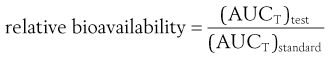 (21.7)
where (AUCT)test and (AUCT)standard are the total areas under the plasma concentration-time curves following the administration of a single dose of the test dosage form and of the standard dosage form, respectively.
When different doses of the test and standard dosage forms are administered, a correction for the size of dose is made as follows:
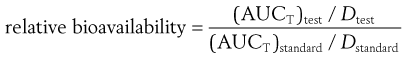 (21.8)
where Dtest and Dstandard are the sizes of the single doses of the test and standard dosage forms, respectively.
Like absolute bioavailability, relative bioavailability may be expressed as a fraction or as a percentage. Urinary excretion data may also be used to measure relative bioavailability as follows:
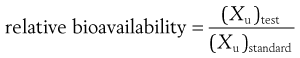 (21.9)
where (Xu)test and (Xu)standard are the total cumulative amounts of unchanged drug ultimately excreted in the urine following the administration of single doses of the test dosage form and the standard dosage form, respectively. If different doses of the test and standard dosage forms are administered on separate occasions, the total amounts of unchanged drug ultimately excreted in the urine per unit dose of drug must be used in this equation.
It should be noted that measurements of relative and absolute bioavailability based on urinary excretion data may also be made in terms of either the total amounts of principal drug metabolite or of unchanged drug plus its metabolites ultimately excreted in the urine. However, the assessment of relative and absolute bioavailability in terms of urinary excretion data is based on the assumption that the total amount of unchanged drug (and/or its metabolites) ultimately excreted in the urine is a reflection of the total amount of intact drug entering the systemic circulation (as discussed in the earlier section on cumulative urinary excretion curves).
Relative bioavailability measurements are often used to determine the effects of dosage form differences on the systemic bioavailability of a given drug. Numerous dosage form factors can influence the bioavailability of a drug. These include the type of dosage form (e.g. tablet, solution, suspension, hard gelatin capsule), differences in the formulation of a particular type of dosage form, and manufacturing variables employed in the production of a particular type of dosage form. A more detailed account of the influence of these factors on bioavailability is given in Chapter 20.
Bioequivalence
An extension of the concept of relative bioavailability, which essentially involves comparing the total amounts of a particular drug that are absorbed intact into the systemic circulation from a test and a recognized standard dosage form, is that of determining whether test and standard dosage forms containing equal doses of the same drug are equivalent or not in terms of their systemic availabilities (i.e. rates and extents of absorption). This is called bioequivalence.
Two or more chemically equivalent products, i.e. products containing equal doses of the same therapeutically active ingredient(s) are said to be bioequivalent if they do not differ significantly in their bioavailability characteristics when administered in the same dose under similar experimental conditions. Hence, in those cases where bioavailability is assessed in terms of plasma concentration-time curves, two or more drug products may be considered bioequivalent if there is no significant difference between any of the following parameters: maximum plasma concentration (Cmax), time to peak height concentration (Tmax) and area under the plasma concentration-time curve (AUC).
In conducting a bioequivalence study, it is usual for one of the chemically equivalent drug products under test to be a clinically proven, therapeutically effective product that serves as a standard against which the other ‘test’ products may be compared. If a test product and the standard product are found to be bioequivalent then it is reasonable to expect that the test product will also be therapeutically effective, i.e. the test and the reference products are therapeutically equivalent. Bioequivalence studies are therefore important in determining whether chemically equivalent drug products manufactured by different companies are therapeutically equivalent, i.e. each will produce identical therapeutic responses in patients.
If two drug products are absolutely bioequivalent, their plasma concentration-time and/or cumulative urinary excretion curves would be superimposable. In such a case there would be no problem in concluding that these products were bioequivalent. Nor would there be a problem in concluding bioinequivalence if the parameters associated with the plasma concentration-time and/or cumulative urinary excretion profiles for the test differed from the standard product by, for instance, 50%. However, a problem arises in deciding whether the test and standard drug products are bioequivalent when such products show relatively small differences in their plasma concentration-time curves and/or cumulative urinary excretion curves.
The problem is, how much of a difference can be allowed between two chemically equivalent drug products still to permit them to be considered bioequivalent? Should this be 10%, 20%, 30% or more? The magnitude of the difference that could be permitted will depend on the significance of such a difference on the safety and therapeutic efficacy of the particular drug. This will depend on such factors as the toxicity, the therapeutic range and the therapeutic use of the drug. In the case of a drug with a wide therapeutic range, the toxic effects of which occur only at relatively high plasma concentrations, chemically equivalent products giving quite different plasma concentration-time curves (Fig. 21.14) may still be considered satisfactory from a therapeutic point of view, although they are not strictly bioequivalent.
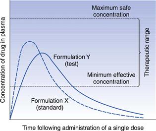
In the case of the hypothetical example shown in Figure 21.14, provided that the observed difference in the rates of absorption (as assessed by the times of peak plasma concentration), and hence in the times of onset, for formulations X and Y is not considered to be therapeutically significant, both formulations may be considered to be therapeutically satisfactory. However, if the drug in question was a hypnotic, in which case the time of onset for the therapeutic response is important, then the observed difference in the rates of absorption would become more important and the two formulations may be considered to be non-equivalent.
If the times of peak plasma concentration for formulations X and Y were 0.5 and 1.0 hour, respectively, it is likely that both formulations would still be deemed to be therapeutically satisfactory despite a 100% difference in their times of peak plasma concentration. However, if the times of peak plasma concentration for formulations X and Y were 2 and 4 hours, respectively, these formulations might no longer be regarded as being therapeutically equivalent even though the percentage difference in their peak plasma concentration was the same.
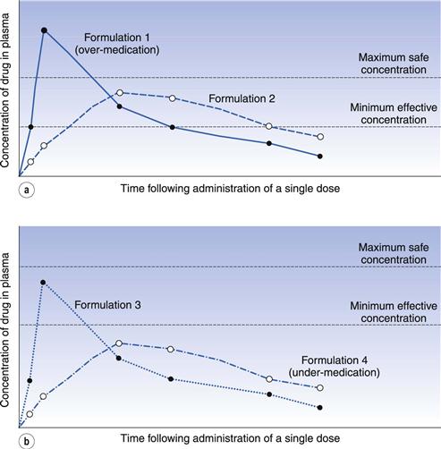
It is difficult to quote a universally acceptable percentage difference that can be tolerated before two chemically equivalent drug products are regarded as being bioinequivalent and/or therapeutically inequivalent. In the case of drug products containing a drug which exhibits a narrow range between its minimum effective plasma concentration and its maximum safe plasma concentration (e.g. digoxin), the concept of bioequivalence is fundamentally important, as in such cases small differences in the plasma concentration-time curves of chemically equivalent drug products may result in patients being over-medicated (i.e. exhibiting toxic responses) or under-medicated (i.e. experiencing therapeutic failure). These two therapeutically unsatisfactory conditions are illustrated in Figure 21.15a and b, respectively.
Despite the problems of putting a value on the magnitude of the difference that can be tolerated before two chemically equivalent drug products are deemed to be bioinequivalent, a value of 20% for the tolerated difference can be regarded as a general criterion for determining bioequivalence. Thus, if all the major parameters in either the plasma concentration-time or cumulative urinary excretion curves for two or more chemically equivalent drug products differ from each other by less than 20%, these products could be judged to be bioequivalent. However, if any one or more of these parameters differ by more than 20% then there might be a problem with the bioequivalence of the test product(s) with respect to the standard product. However, recently some regulatory authorities have been adopting more stringent requirements for bioequivalence, involving statistical models and considerations of average, population and individual pharmacokinetics.
A further crucial factor in establishing bioequivalence, or in determining the influence that the type of dosage form, route of administration, etc., have on the bioavailability of a given drug, is the proper design, control and interpretation of such experimental studies.
Assessment of site of release in vivo
There are many benefits of being able to assess the fate of a dosage form in vivo and the site and release pattern of the drug. Particularly for drugs that show poor oral bioavailability, or in the design and development of controlled- or sustained-release delivery systems, the ability to follow the transit of the dosage form and the release of drug from it is advantageous. The technique of gamma-scintigraphy is now used extensively and enables a greater knowledge and understanding to be gained of the transit and fate of pharmaceuticals in the gastrointestinal tract.
Gamma (γ)-scintigraphy is a versatile, non-invasive and ethically acceptable technique that is capable of obtaining information both quantitatively and continuously. The technique involves the radiolabelling of a dosage form with a γ-emitting isotope of appropriate half-life and activity. Technetium-99m is often the isotope of choice for pharmaceutical studies because of its short half-life (6 hours). The radiolabelled dosage form is administered to a subject who is positioned in front of a γ-camera. γ-Radiation emitted from the isotope is focused by a collimator and detected by a scintillation crystal and its associated circuitry. The signals are assembled by computer software to form a two-dimensional image of the dosage form in the gastrointestinal tract. The anatomy of the gastrointestinal tract can be clearly seen from liquid dosage forms, and the site of disintegration of solid dosage forms identified. The release of the radiolabel from the dosage form can be measured by following the intensity of the radiation. By co-administration of a radiolabelled marker and a drug in the same dosage form, and simultaneous imaging and the taking of blood samples, the absorption site and release rate of a drug can be determined (for example with the InteliSite capsule described earlier in this chapter). When used in this way, the technique is often referred to as pharmacoscintigraphy.
Biopharmaceutics Classification System
As a result of the plethora and variability of biopharmaceutical properties of existing and potential drugs, an attempt has been made to classify drugs into a small number of categories. A scientific basis for a Biopharmaceutics Classification System (BCS) has been proposed that classifies drugs into four classes according to their dose, their aqueous solubility across the gastrointestinal pH range and their permeability across the gastrointestinal mucosa.
The scheme was originally proposed for the identification of immediate-release solid oral products for which in vivo bioequivalence tests may not be necessary. It is also useful to classify drugs and predict bioavailability issues that may arise during the various stages of the development process and is now utilized widely by many regulatory authorities.
The four classes are defined in terms of high and low aqueous solubility and high and low permeability:
• Class I – high solubility/high permeability
• Class II – low solubility/high permeability
A drug is considered to be highly soluble where the highest dose strength is soluble in 250 mL or less of aqueous media over the pH range 1–8. The volume is derived from the minimum volume anticipated in the stomach when a dosage form is taken in the fasted state with a glass of water. If the volume of aqueous media needed to dissolve the drug in pH conditions ranging from 1 to 8 is greater than 250 mL then the drug is considered to have low solubility. The classification therefore takes into account the dose of the drug as well as its solubility.
A drug is considered to be highly permeable when the extent of absorption in humans is expected to be greater than 90% of the administered dose. Permeability can be assessed using one of the methods discussed earlier in this chapter that has been calibrated with known standard compounds or by pharmacokinetic studies.
Class I drugs.
Class I drugs will dissolve rapidly when presented in immediate-release dosage forms, and are also rapidly transported across the gut wall. Therefore (unless they form insoluble complexes, are unstable in gastric fluids or undergo presystemic clearance) it is expected that such drugs will be rapidly absorbed and thus show good bioavailability. Examples of class I drugs are the β-blockers propranolol and metoprolol.
Class II drugs.
In contrast, for drugs in class II, the dissolution rate is liable to be the rate-limiting step in oral absorption. For class II drugs it should therefore be possible to generate a strong correlation between in vitro dissolution and in vivo absorption (discussed earlier in this chapter). Examples of class II drugs are the non-steroidal anti-inflammatory drug ketoprofen and the antiepileptic carbamazepine. This class of drug should be amenable to formulation approaches to improve the dissolution rate and hence oral bioavailability.
Class III drugs.
Class III drugs are those that dissolve rapidly but which are poorly permeable. Examples are the H2-antagonist ranitidine and the β-blocker atenolol. It is important that dosage forms containing class III drugs release them rapidly in order to maximize the amount of time these drugs, which are slow to permeate the gastrointestinal epithelium, are in contact with it.
Class IV drugs.
Class IV drugs are those that are classed as poorly soluble and poorly permeable. These drugs are liable to have poor oral bioavailability, or the oral absorption may be so low that they cannot be given by the oral route. The diuretics hydrochlorothiazide and furosemide are examples of class IV drugs. Forming prodrugs of class IV compounds, the use of novel drug delivery technologies or finding an alternative route of delivery are approaches that have to be adopted to significantly improve their absorption into the systemic circulation.
Summary
This chapter discusses a range of approaches to assessing the biopharmaceutical properties of drugs that are intended for oral administration. Methods of measuring and interpreting bioavailability data are also described. The concepts of bioequivalence and the Biopharmaceutics Classification System of drugs are introduced.
It is imperative that the biopharmaceutical properties of drugs are fully understood, both in the selection of candidate drugs during the discovery process and in the design and development of efficacious immediate- and controlled-release dosage forms.
References
1. Artusson P, Palm K, Luthman K. Caco-2 monolayers in experimental and theoretical predictions of drug transport Advanced Drug Delivery. Reviews. 1996;22:67–84.
2. Yang Y, Yu LX. Oral drug absorption, evaluation and prediction. In: Qiu Y, Chen Y, Zhang GGZ, Liu L, Porter WR, eds. Developing Solid Oral Dosage Forms: Pharmaceutical Theory and Practice. London: Academic Press; 2009.
Bibliography
1. Dickinson PA, Lee WW, Stott PW, et al. Clinical relevance of dissolution testing in Quality by Design. American Association of Pharmaceutical Scientists Journal. 2008;10:380–390.
2. Ehrhardt Carsten, Kim Kwang-jin. Drug Absorption Studies; in situ, in vitro and in silico Models. New York: Springer; 2008.
3. Selen A, Cruañes MT, Müllertz A, et al. Conference Report: Applied Biopharmaceutics and Quality by Design for Dissolution/Release Specification Setting: Product Quality for Patient Benefit. American Association of Pharmaceutical Scientists Journal. 2010;12:465–472.