Chapter 8 Ankle, Foot, and Lower Leg Ultrasound
 Additional videos for this topic are available online at www.expertconsult.com.
Ankle and Foot Anatomy
Osseous Anatomy
The ankle joint is a hinged synovial articulation between the talus and the distal tibia and the fibula (Fig. 8-1). Inferiorly, the talus articulates with the calcaneus through three facets, joined by the cervical and interosseous talocalcaneal ligaments located in a cone-shaped region termed the sinus tarsi, which opens laterally.1 The Chopart joint represents the articulations between the talus and navicular and the calcaneus and cuboid bones. The navicular, in turn, articulates with the medial, middle, and lateral cuneiforms, which then articulate with the first through third metatarsals. The fourth and fifth metatarsals articulate directly with the cuboid bone, and the tarsometatarsal articulations collectively are called the Lisfranc joint. Phalangeal bones extend beyond the metatarsals.
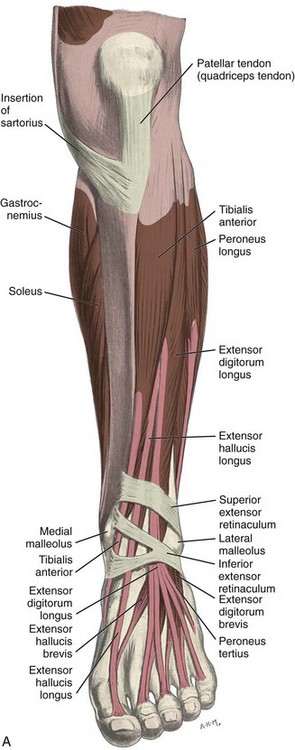
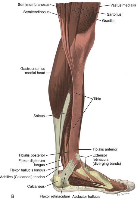
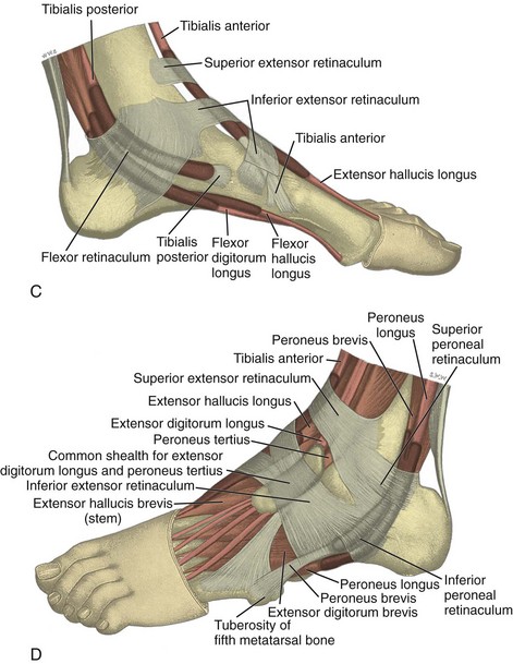
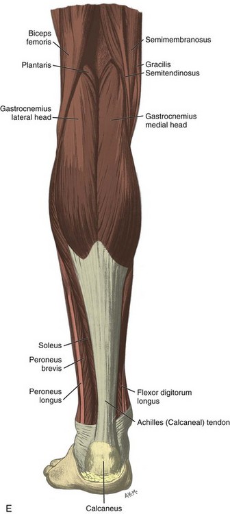
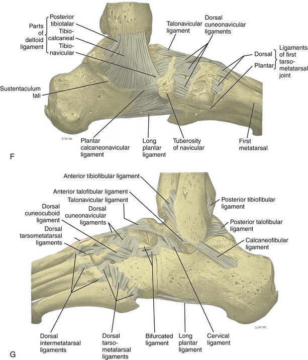
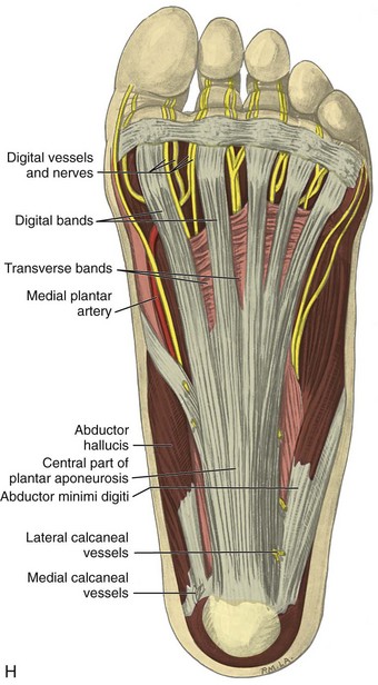
FIGURE 8-1 Leg, ankle, and foot anatomy.
(A and E, From Schaefer, EA, Symington J, Bryce TH [eds]: Quain’s anatomy, 11th ed, London, 1915, Longmans, Green, with permission from Pearson Education; B, C, D, and H, from Standring S: Gray’s anatomy: the anatomical basis of clinical practice, 39th ed, Edinburgh, 2005, Churchill Livingstone; F and G, drawn from a specimen in the Museum of the Royal College of Surgeons of England, with permission from the Council.)
Muscle and Tendon Anatomy
Anteriorly, from medial to lateral, are the tibialis anterior (origin: proximal tibia and interosseous membrane; insertion: base of first metatarsal and medial cuneiform), the extensor hallucis longus (origin: fibula and interosseous membrane; insertion: distal phalanx of the first digit), and the extensor digitorum longus tendons (origin: tibia, fibula, and interosseous membrane; insertion: phalanges of the second through fifth digits) (see Fig. 8-1A to C). The peroneus tertius extends from the fibula and interosseous membrane to the base of the fifth metatarsal. The anterior tendons are held in place by the superior and inferior extensor retinacula. The anterior tibial artery courses beneath the superior extensor retinaculum and becomes the dorsalis pedis artery, located between the extensor hallucis and extensor digitorum longus tendons. The deep peroneal nerve follows the anterior tibial artery and dorsal pedis and bifurcates as medial and lateral branches anterior to the ankle.
Medially, from anterior to posterior, are the tibialis posterior (origin: tibia, fibula, and interosseous membrane; insertion: navicular, cuneiforms, and second through fourth metatarsals), the flexor digitorum longus (origin: tibia; insertion: distal phalanges of second through fifth digits), and the flexor hallucis longus tendons (origin: fibula; insertion: base of distal phalanx of first digit) (see Fig. 8-1A to D). Between the flexor digitorum and flexor hallucis longus tendons at the posterior ankle are the tibial nerve and posterior tibial artery and veins. The order of structures from anterior to posterior from the medial malleolus can be remembered with the phrase “Tom, Dick, And Very Nervous Harry” (T, Tibialis posterior tendon; D, flexor Digitorum longus tendon; A, tibial Artery; V, tibial Veins; N, tibial Nerve; and H, flexor Hallucis longus tendon). The flexor retinaculum extends from the medial malleolus to the calcaneus superficial to the medial tendons and tibial nerve, which forms the roof of the tarsal tunnel. The tibial nerve divides into medial and lateral plantar nerves and a smaller medial calcaneal nerve.2 The inferior calcaneal nerve usually originates from the medial plantar branch and courses between the abductor hallucis and quadratus plantae muscles and then adjacent to the calcaneus.3 The medial and lateral plantar nerves continue toward the digits as the common plantar digital nerves and then as the proper plantar digital nerves. More distally under the mid-foot, the flexor digitorum and flexor hallucis longus tendons cross each other, a configuration termed the knot of Henry. The flexor digitorum and flexor hallucis brevis muscles are located in the plantar aspect of the foot.
Laterally, the peroneus brevis (origin: distal fibula; insertion: fifth metatarsal base) and peroneus longus tendons (origin: proximal fibula and tibial condyle; insertion: first metatarsal base and medial cuneiform) are found posterior to the fibula (see Fig. 8-1A, B, D, and E). The musculotendinous junction of the peroneus longus is more superior to that of the peroneus brevis; at the level of the distal fibula, the peroneus brevis muscle and tendon are found medial and anterior to the tendon of the peroneus longus. More distally, the peroneus brevis tendon is typically in contact with the posterior fibular or retromalleolar groove. The normal peroneus muscle belly should taper so that only tendon is present at the fibula tip.4 The peroneal tendons are held in place by the superior and inferior peroneal retinacula.5 The peroneal tendons then course anteriorly on each side of the peroneal tubercle of the calcaneus and extend to their insertions. As a normal variant, an accessory tendon called the peroneus quartus may be found posterior to the fibula; this tendon most commonly originates from the peroneus brevis and inserts on the lateral aspect of the calcaneus at the retrotrochlear eminence.6 Over the lateral aspect of the calcaneus, the extensor digitorum brevis muscle originates from the calcaneus and extensor retinaculum and inserts distally on the second through fifth phalanges.
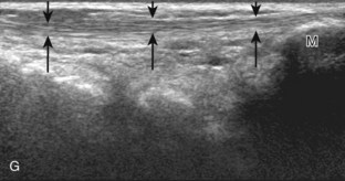
Posteriorly in the calf, the medial and lateral heads of the gastrocnemius muscle converge with the soleus to form the Achilles tendon (termed the triceps surae), which inserts onto the calcaneus (see Fig. 8-1B and E).7 The plantaris muscle originates from the lateral femur, courses obliquely through the popliteal region, continues as a thin tendon between the muscle bellies of the medial head of the gastrocnemius and soleus muscles, courses distally at the medial aspect of the Achilles tendon, and then inserts onto the calcaneus. At the plantar aspect of the calcaneus, the plantar aponeurosis originates from the medial calcaneus and extends distally as medial, central, and lateral cords (see Fig. 8-1H). The central cord envelops the flexor digitorum brevis muscle.
Ligamentous Anatomy
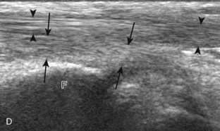
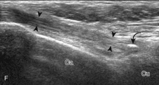
The stabilizing structures of the lateral ankle include the anterior talofibular ligament, which extends from the fibular to the talus in the transverse plane; the calcaneofibular ligament, which extends from the fibula inferiorly and posteriorly to the calcaneus deep to the peroneal tendons; and the posterior talofibular ligament, which extends from the fibula to the posterior aspect of the tibia in the transverse plane (see Fig. 8-1G).8 In addition, the anterior and posterior tibiofibular ligaments extend laterally and inferiorly in an oblique fashion from the tibia to the fibula. An accessory anterior tibiofibular ligament may be present, also called Bassett ligament.9 At the medial aspect of the ankle, the deltoid ligament is found, consisting of deep (anterior tibiotalar and posterior tibiotalar) and superficial (tibiocalcaneal and tibionavicular) components (see Fig. 8-1F).8 The spring ligament complex consists of superomedial, medioplantar, and inferoplantar calcaneonavicular ligaments.10 In addition to other small ligaments that connect the various tarsal bones and are named by their osseous attachments, the Lisfranc ligament proper is a strong ligament that connects obliquely from the medial cuneiform to the base of the second metatarsal bone.11 The bifurcate ligament extends from the calcaneus to the navicular and cuboid bones at the lateral aspect of the mid-foot.
Ultrasound Examination Technique
Table 8-1 is a checklist for ankle, calf, and forefoot ultrasound examination. Examples of diagnostic ankle ultrasound reports are available online at www.expertconsult.com (see eBox 8-1 and 8-2).
TABLE 8-1 Ankle, Calf, and Forefoot Ultrasound Examination Checklist
| Location | Structures of Interest |
|---|---|
| Ankle: anterior |
eBox 8-1 Sample Diagnostic Ankle Ultrasound Report
Normal
Examination: Ultrasound of the Right Ankle
History: Pain, evaluate for tendon tear
Findings: No evidence of ankle joint effusion. Anteriorly, the tibialis anterior, extensor hallucis longus, and extensor digitorum longus are normal. Medially, the tibialis posterior, flexor digitorum longus, flexor hallucis longus, tibial nerve, and deltoid ligament are normal. Laterally, the peroneus brevis and longus are normal, as are the anterior talofibular, calcaneofibular ligament, and anterior tibiofibular ligaments. Posteriorly, the Achilles tendon and plantar fascia are normal. Focused ultrasound examination directed by patient symptoms over the lateral ankle revealed no abnormality.
Impression: Unremarkable ultrasound examination of the right ankle. No tendon abnormality.
eBox 8-2 Sam.ple Diagnostic Ankle Ultrasound Report
Abnormal
Examination: Ultrasound of the Right Ankle
History: Pain, evaluate for tendon tear
Findings: There is a small ankle joint effusion. No synovial hypertrophy. Laterally, there is abnormal anechoic fluid and hypoechoic synovial hypertrophy surrounding the peroneal tendons at the level of the distal fibula. A longitudinal tear is seen in the peroneus brevis. The superior peroneal retinaculum is torn at the fibula, and peroneal tendon dislocation occurs with dynamic evaluation in ankle dorsiflexion and eversion. No low-lying peroneus brevis muscle. Otherwise, the anterior talofibular, calcaneofibular ligament, and anterior tibiofibular ligaments.
Anteriorly, the tibialis anterior, extensor hallucis longus, and extensor digitorum longus are normal. Medially, the tibialis posterior, flexor digitorum longus, flexor hallucis longus, tibial nerve, and deltoid ligament are normal.
Posteriorly, the Achilles tendon and plantar fascia are normal. Focused ultrasound examination directed by patient symptoms over the lateral ankle corresponded to the peroneal tendon tear.
Anterior Ankle Evaluation
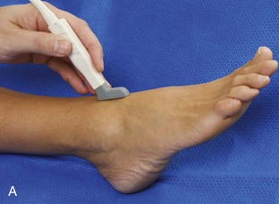
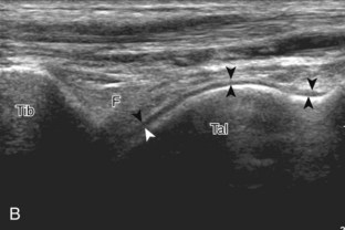
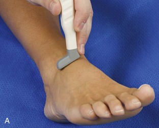
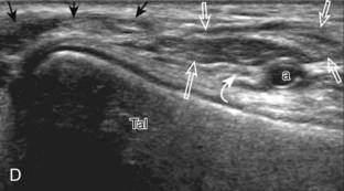
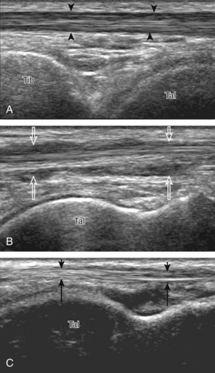
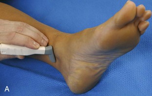
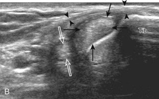
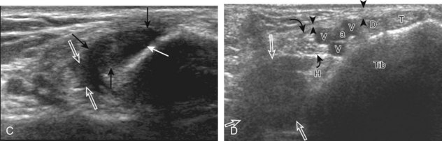
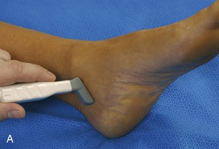
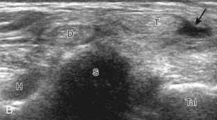
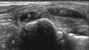
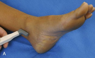
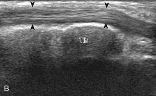
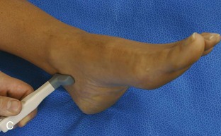
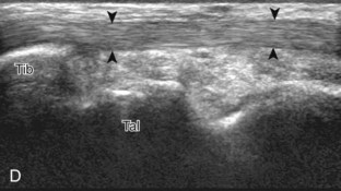
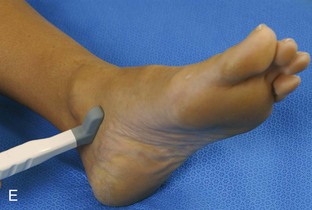
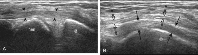
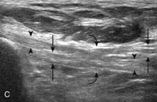
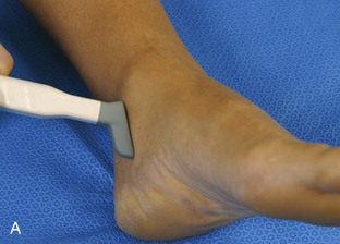
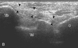
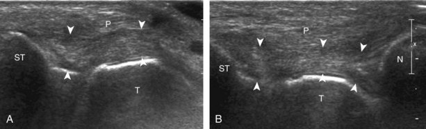
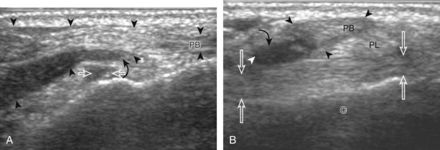
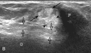
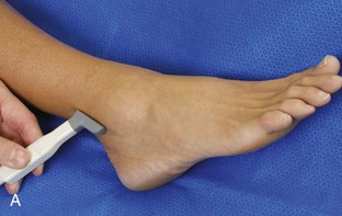
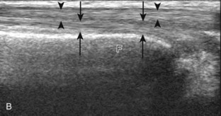
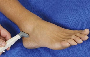
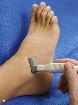
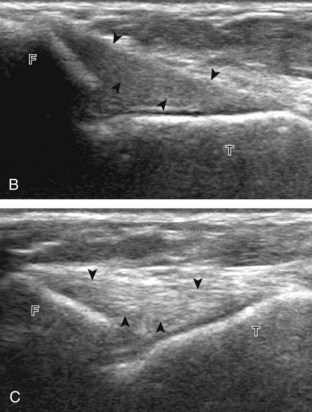
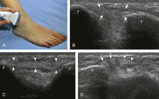
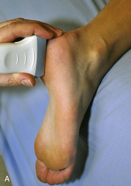
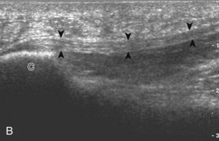
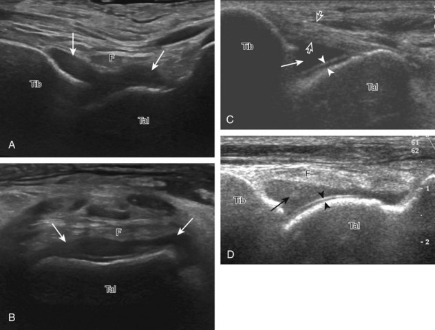
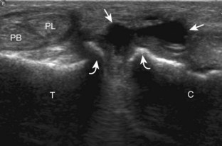
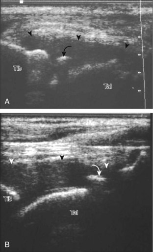
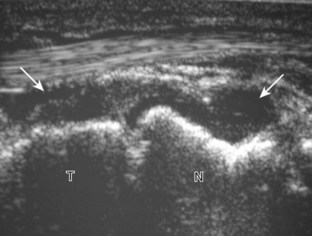
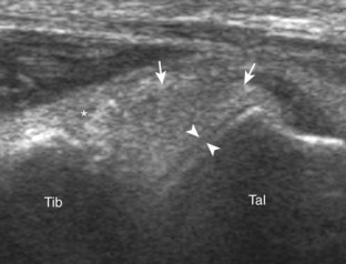
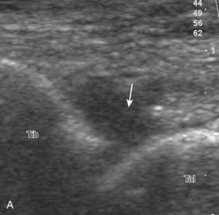
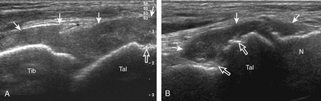
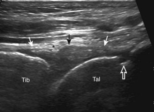
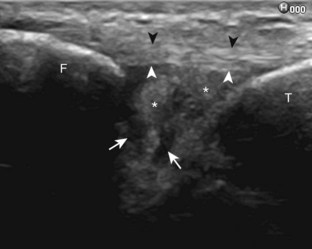
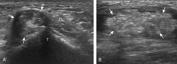
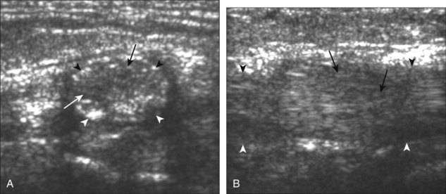
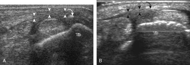
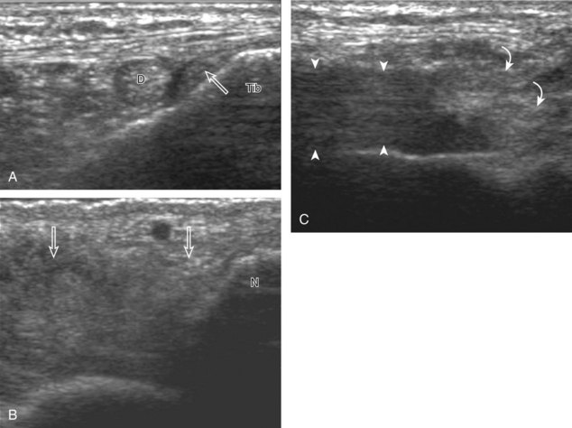
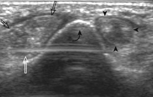
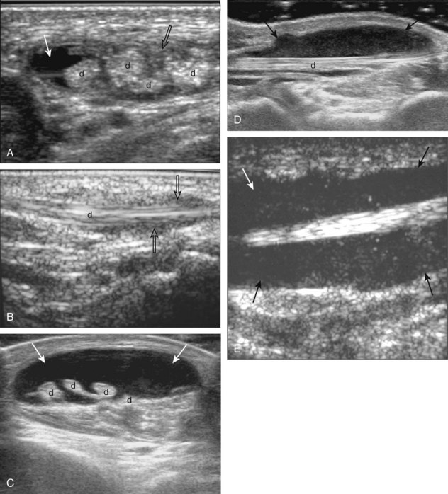
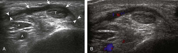
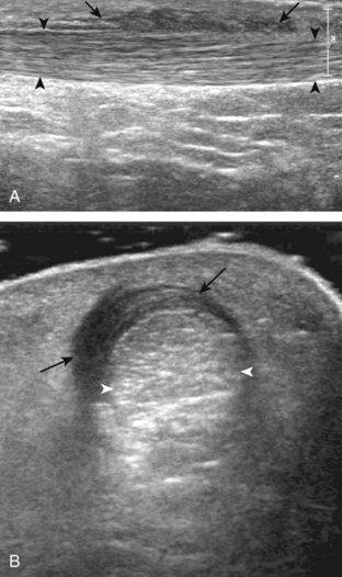
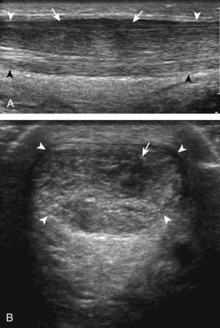
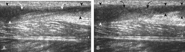
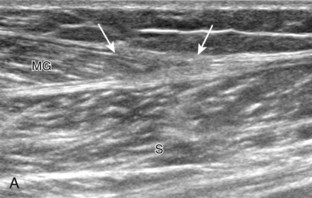
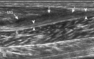
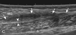
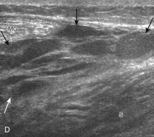
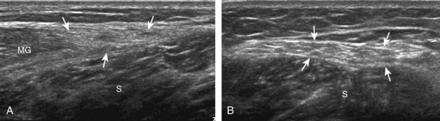
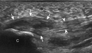
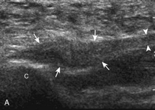
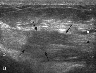
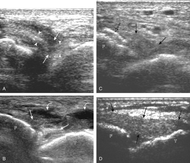
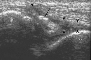
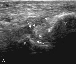
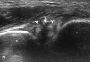
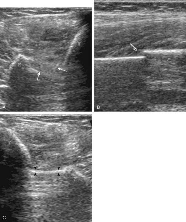
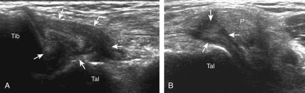
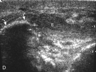
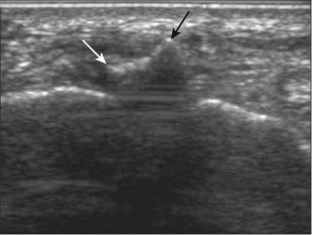
The primary structures evaluated from the anterior approach are the anterior ankle joint recess, the tibialis anterior, the extensor hallucis longus, the dorsalis pedis artery and superficial peroneal nerve, and the extensor digitorum longus. The transducer is first placed in the sagittal plane at the level of the tibiotalar joint with the foot in mild plantar flexion (Fig. 8-2A). The hyperechoic bone landmarks of the distal tibia and proximal talus are used for orientation, and the anterior ankle joint region is evaluated for joint abnormality (see Fig. 8-2B). It is important to evaluate not only the anterior joint recess in the sagittal plane but also the parasagittal plane laterally near the anterior talofibular ligament because small amounts of joint fluid may be present only at this site. Next, to evaluate the anterior tendons, the transducer is placed transversely at the level of the ankle joint (Fig. 8-3A). It is important to begin in the transverse plane, short axis to the tendons so that each of the tendons can be accounted for and differentiated from each other as they may appear similar in long axis. The tibialis anterior tendon is the largest, located most medially, with the typical hyperechoic and fibrillar echotexture (see Fig. 8-3B). One may toggle the transducer (see Fig. 1-5B) to assist in identification of the tendons in short axis. This maneuver causes the normally hyperechoic tendon to appear artifactually hypoechoic from anisotropy, which will make the tendon more conspicuous surrounded by the hyperechoic fat (see Fig. 8-3C). Lateral to the tibialis anterior is the extensor hallucis longus (see Fig. 8-3D). The muscle belly of this structure extends more inferiorly compared with the other anterior tendons, and this hypoechoic muscle tissue should not be mistaken for tenosynovitis. The adjacent anterior tibial artery is seen as it crosses from medial to lateral deep to the extensor hallucis longus, which continues as the dorsal pedis artery once beyond the superior extensor retinaculum. The next lateral structure is the extensor digitorum longus with its multiple tendons that extend distally to the digits (see Fig. 8-3D and E). Lateral to this, the peroneus tertius extends to the fifth metatarsal base. Each of these structures should then be evaluated in long axis from proximal to the ankle joint to at least the mid-foot region, the extent of which can be guided by physical examination findings or patient history (Fig. 8-4). For identification of the deep peroneal nerve, the anterior tibial artery is an ideal landmark (Fig. 8-5); when moving the transducer from proximal to distal over the anterior tibial artery in short axis, the deep peroneal nerve is identified as it crosses from medial to lateral over the anterior tibial artery.
Medial Ankle Evaluation
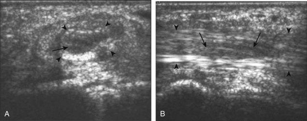
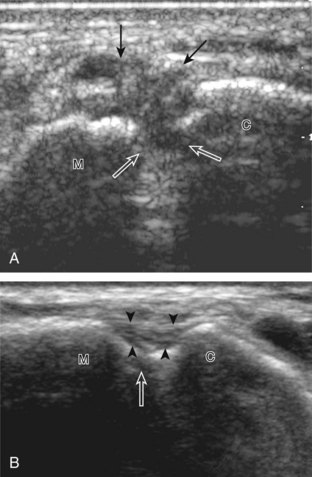
For medial evaluation, the supine patient externally rotates at the hip or rolls partially onto the ipsilateral side to gain access to the medial aspect of the ankle. Ultrasound examination begins in the transverse plane superior to the medial malleolus (Fig. 8-6A). The hyperechoic and shadowing surface of the tibia is seen, and the transducer is moved posteriorly. The first tendon identified is the tibialis posterior tendon in short axis (see Fig. 8-6B). One may toggle the transducer (see Fig. 1-3B) to assist in identification of the tendons in short axis, which causes the tendon to appear hypoechoic from anisotropy and improves conspicuity compared with the adjacent hyperechoic fat (see Fig. 8-6C). The transducer is then moved posteriorly to identify the flexor digitorum longus tendon, the posterior tibial artery and veins, the tibial nerve, and then the flexor hallucis longus tendon in order from anterior to posterior (see Fig. 8-6D). The tibialis posterior tendon is typically twice the size of the adjacent flexor digitorum longus tendon. The thin and hyperechoic flexor retinaculum can also be identified superficial to the tendons, and it attaches to the tibia.
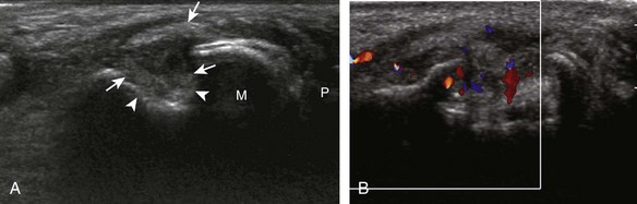
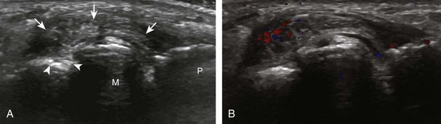
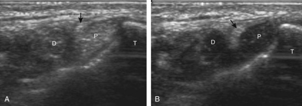
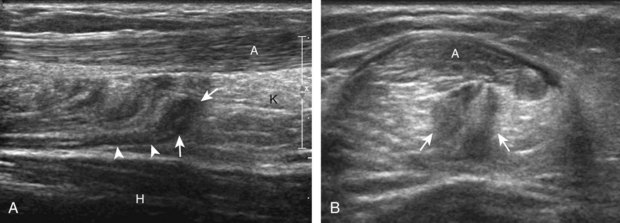
Evaluation is continued distally with the transducer short axis to each tendon; the transducer is rotated to the coronal plane as each tendon is followed distally (Fig. 8-7A). Anisotropy is again used to help delineate each tendon in short axis (see Fig. 8-7B and C). At the medial aspect of the calcaneus, a bony protuberance called the sustentaculum tali protrudes medially to articulate with the talus as the middle facet of the anterior subtalar joint. The medial tendons have characteristic locations relative to the sustentaculum tali (see Fig. 8-7B). The tibialis posterior tendon is dorsal and superficial, the flexor digitorum longus lies immediately superficial, and the flexor hallucis longus tendon lies plantar to the sustentaculum tali in a bony groove of the calcaneus.
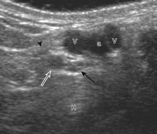
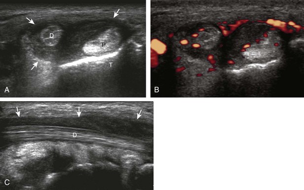
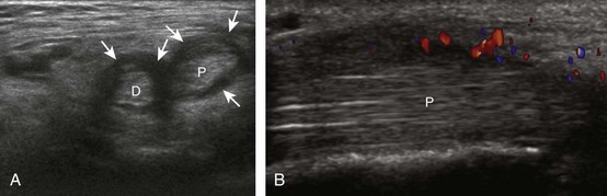
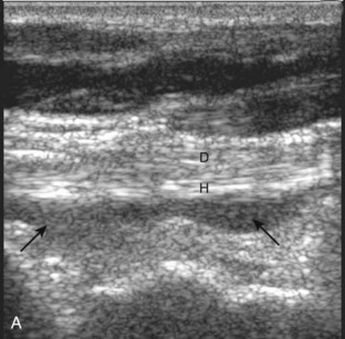
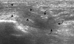
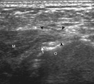
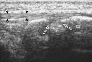
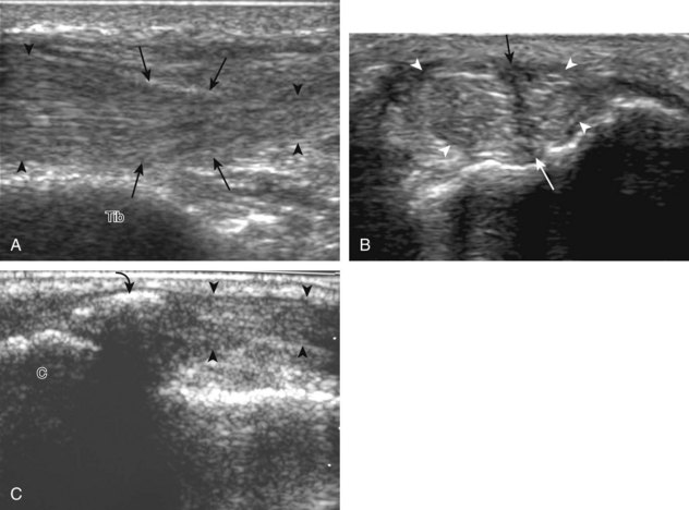
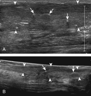
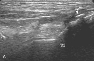
In the supramalleolar region, the tibial nerve is located between the flexor digitorum longus and flexor hallucis longus tendons. In cross section, the individual hypoechoic nerve fascicles surrounded by hyperechoic connective tissue take on a honeycomb appearance (see Fig. 8-6D), whereas in long axis a fascicular pattern is appreciated that, in contrast to adjacent tendons, is coarser in echotexture. In the supramalleolar region, a small medial calcaneal nerve arising from the tibial nerve can be identified; this branch courses directly inferior, medial to the calcaneus (Fig. 8-8). The tibial nerve then divides into medial and lateral plantar branches, which continue under the mid-foot to give off the common plantar digital nerves and then the proper plantar digital branches.
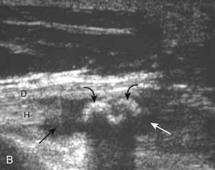
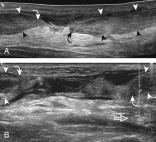
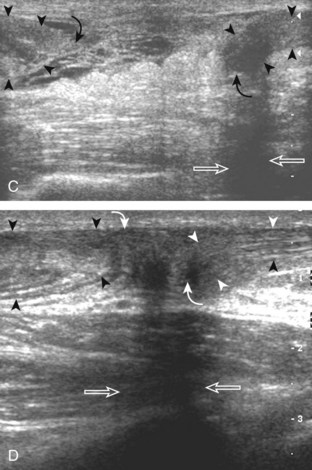
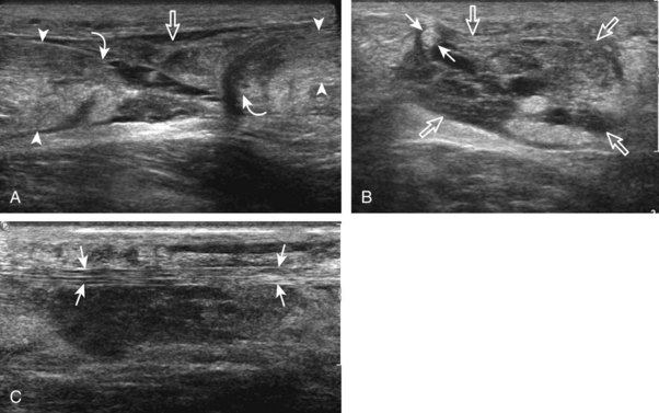
To assess for medial tendon abnormality in long axis, the transducer is then moved back to the level of the distal tibia over the tibialis posterior tendon and is turned 90 degrees (Fig. 8-9A and B). As the transducer follows the course of the tibialis posterior tendon in long axis, the transducer moves from a coronal plane relative to the body to the axial plane (see Fig. 8-9C to F). At the navicular bone, it is common to visualize mild thickening and decreased echogenicity of the distal tibialis posterior tendon, related to its insertion on the talus and anisotropy from several of the tibialis posterior tendon fibers that course plantar to the navicular to insert at the cuneiforms and the second through fourth metatarsals (see Fig. 8-9F). It is also common to see a small amount of fluid within the tendon sheath of the tibialis posterior tendon just beyond the medial malleolus, usually seen only along one side of the tendon; asymptomatic fluid should not be present at the navicular where a tendon sheath is absent.12 An accessory navicular bone may be seen within the distal tibialis posterior tendon near the navicular bone (see Fig. 8-79). To assess the flexor digitorum longus tendon, examination again begins transversely superior and posterior to the medial malleolus, followed by assessment in long axis and distally (Fig. 8-10A). Similarly, the flexor hallucis longus tendon can be assessed first in short axis and then in long axis (see Fig. 8-10B). As the flexor digitorum longus and flexor hallucis longus tendons are followed distally beneath the mid-foot, the two tendons cross, called the knot of Henry (see Fig. 8-10C).
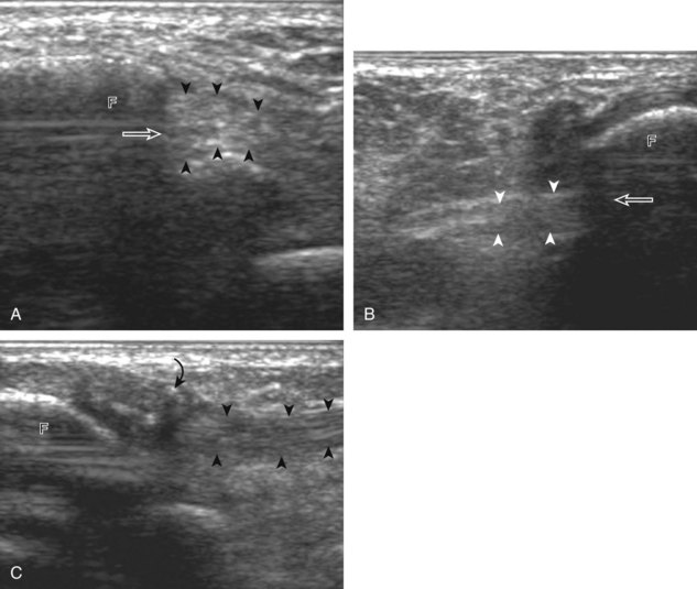
After assessment of the medial tendons, the components of the deltoid ligament are evaluated. The transducer is initially placed in the coronal plane at the medial malleolus (Fig. 8-11A). At this location, a superficial hyperechoic and fibrillar tibiocalcaneal component of the deltoid ligament is identified, extending from the tibia to the calcaneus (see Fig. 8-11B). With rotation of the distal aspect of the transducer anteriorly with the proximal aspect fixed to the medial malleolus, the more superficial tibionavicular and deeper anterior tibiotalar components are identified (see Fig. 8-11C). The distal aspect of the transducer is then rotated posteriorly while the proximal aspect remains fixed to the medial malleolus with the foot in dorsiflexion. In this position, the thick hyperechoic and fibrillar posterior tibiotalar component of the deltoid ligament is identified deep to the tibialis posterior tendon (see Fig. 8-11D).
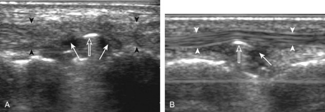
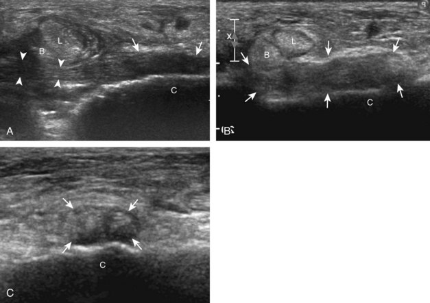
The spring ligament complex consists of superomedial, medioplantar, and inferoplantar calcaneonavicular ligaments.10 To visualize each component, the transducer is initially placed in the transverse plane inferior to the medial malleolus and over the sustentaculum tali. By moving the transducer anteriorly and angling superior toward the talar head, the superomedial calcaneonavicular ligament is identified in long axis between the tibialis posterior tendon and the talus (Fig. 8-12).13
Lateral Ankle Evaluation
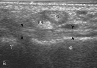
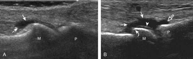
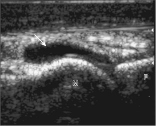
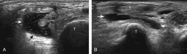
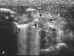
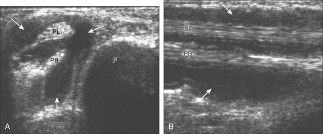
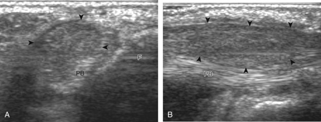
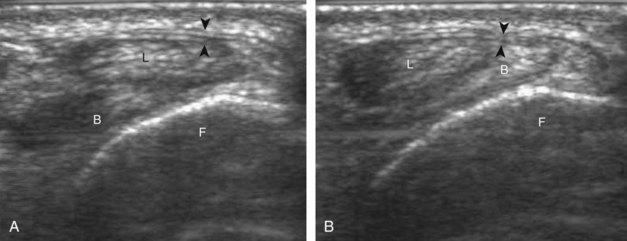
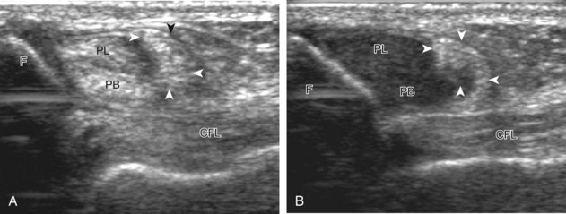
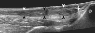
Structures of interest include the peroneal tendons and the lateral ligamentous structures of the ankle. Examination begins in the supramalleolar region in the transverse plane, directly posterior to the fibula in the retromalleolar groove or sulcus (Fig. 8-13A). At this location, the muscle belly and tendon of the peroneus brevis are identified in short axis (see Fig. 8-13B). An adjacent tendon, the peroneus longus is also seen, characterized by lack of a muscle belly at this level. With movement of the transducer from superior to inferior, the normal peroneus brevis muscle belly will taper; only the peroneus brevis and longus tendons should be visible at the extreme fibula tip (see Fig. 8-13C). If the peroneus brevis muscle is present beyond the fibular tip, this normal variation is termed a low-lying muscle belly of the peroneus brevis and may be associated with tendon tear (see Fig. 8-92).4 Although variable, the peroneus brevis is usually directly against the posterior cortex of the fibula, with the adjacent peroneus longus tendon more posterior. The thin and hyperechoic superior peroneal retinaculum can be seen extending over the tendons to insert on the posterolateral margin of the fibula.
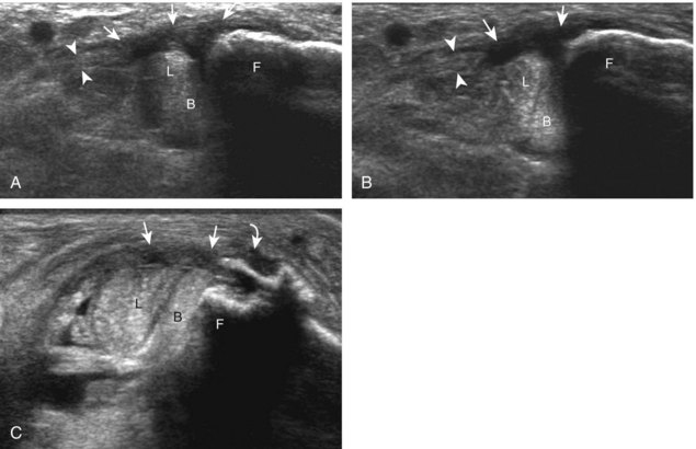
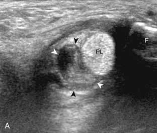
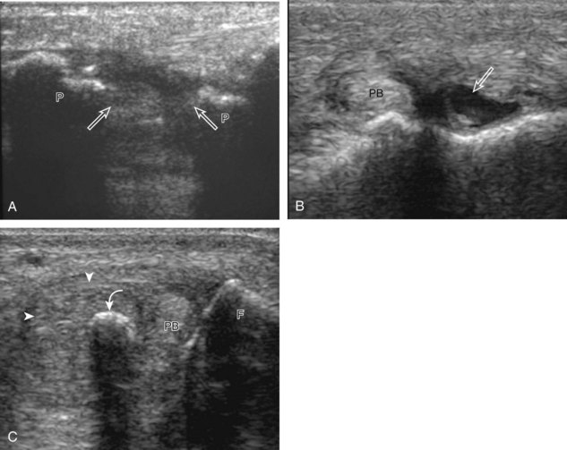
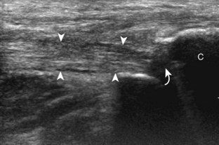
Assessment is continued short axis to the peroneal tendons. Toggling the transducer is a helpful maneuver to identify the tendons in short axis, which causes the tendon to appear hypoechoic from anisotropy and improves conspicuity compared with the adjacent hyperechoic fat (see Fig. 1-12). As the transducer crosses the oblique plane between the tip of the fibular and the posterior aspect of the heel, the normal calcaneofibular ligament can be seen deep to the peroneal tendons (Fig. 8-14). As the peroneal tendons are followed in short axis, the transducer becomes positioned in the coronal plane (Fig. 8-15A). At the lateral aspect of the calcaneus, a bony prominence of variable size called the peroneal tubercle is present (see Fig. 8-15B). At this site, the peroneus brevis and longus tendons diverge into different directions. Because of their different respective orientations at the peroneal tubercle, it is difficult to image both tendons in short axis without one tendon appearing artifactually hypoechoic from anisotropy (see Fig. 8-15B). With minimal clockwise and counterclockwise transducer rotation and toggling, anisotropy of each tendon can be eliminated (see Fig. 8-15C). The peroneus brevis can be followed distally to its insertion on the fifth metatarsal base, and the peroneus longus similarly can be imaged under the mid-foot and forefoot to its insertion on the medial cuneiform and first metatarsal base.
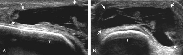
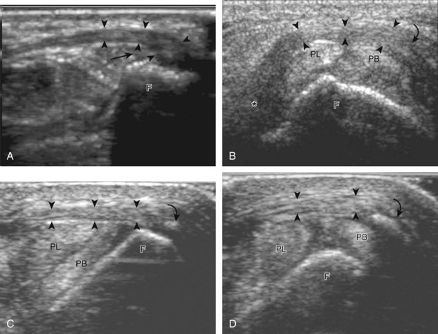
For assessment of the peroneal tendons in long axis, one again returns to the supramalleolar region and places the transducer over the retromalleolar groove with the transducer in the oblique-sagittal plane toward the posterior aspect of the fibula (Fig. 8-16A). This approach allows visualization of the peroneus brevis and longus tendons in one imaging plane (see Fig. 8-16B). As the transducer is moved distally, the tendons begin to diverge distal to the fibula (see Fig. 8-16C and D). At this point, the peroneus longus and brevis are followed individually (see Fig. 8-16E). The peroneus longus courses deep toward the cuboid, where it commonly demonstrates anisotropy (see Fig. 8-16F). An echogenic os peroneum may be seen within the peroneus longus tendon.14 More distal assessment of the peroneus longus may be completed if symptoms warrant. The peroneus brevis tendon can be followed distally from the fibula to its insertion on the base of the fifth metatarsal (see Fig. 8-16G).
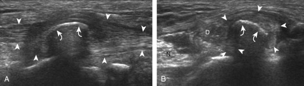
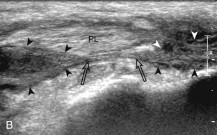
The first lateral ankle ligament to be assessed is the anterior talofibular ligament. For localization, the transducer is first placed directly over the lateral aspect of the distal fibula. The transducer is then moved inferiorly. Once the extreme distal fibula tip is reached, the transducer is moved slightly superiorly and anteriorly to visualize the talus (Fig. 8-17A). In this position, the anterior talofibular ligament appears as a homogeneously hypoechoic structure from anisotropy resulting from the oblique course of the ligament toward the talus (see Fig. 8-17B). The transducer is then angled (heel-toe maneuver) so that the ligament fibers are perpendicular to the sound beam, to eliminate anisotropy, and the normal anterior talofibular ligament is seen as a continuous compact fibrillar structure that extends from the fibula to the talus in long axis (see Fig. 8-17C) (Video 8-1) . Anisotropy is used to one’s advantage in this application because initial identification of the anterior talofibular ligament is enhanced; the hypoechoic ligament is more conspicuous adjacent to the hyperechoic fat. Once the ligament is identified, it is important to eliminate anisotropy to exclude ligament abnormality.
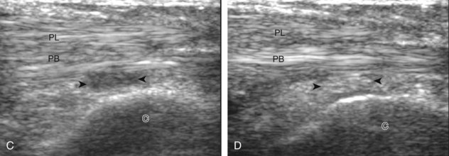
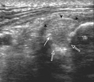
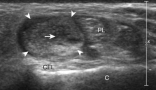
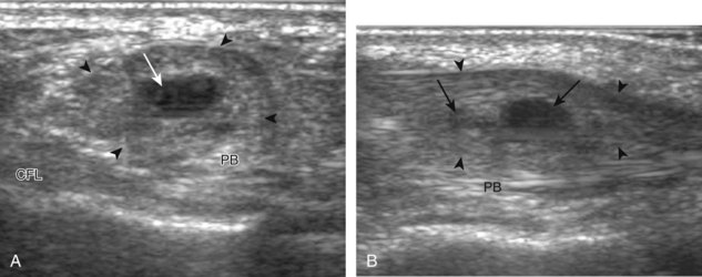
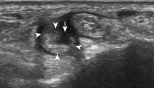
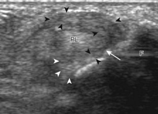
To evaluate the calcaneofibular ligament in long axis, the transducer is placed in an oblique-coronal plane between the fibular tip and the posterior aspect of the heel where the calcaneofibular ligament is identified between the peroneal tendons and calcaneus (Figs. 8-18A and B). The calcaneofibular ligament is often incidentally seen during evaluation of the peroneal tendons in (see Fig. 8-14B). In short axis, the normal calcaneofibular ligament may appear hypoechoic from anisotropy and simulate a complex ganglion cyst associated with the peroneal tendons (see Fig. 8-18C and D).
To evaluate the anterior inferior tibiofibular ligament, the transducer is initially placed in the axial plane over the distal tibia and fibula. As the transducer is moved inferiorly, the cortex of the tibia disappears from view, and the talus appears, a finding that indicates the level of the ankle joint. The transducer is moved superiorly again to identify the most distal aspect of the tibia, and then the lateral aspect of the transducer is rotated inferiorly to visualize the hyperechoic and compact fibrillar anterior inferior tibiofibular ligament, which courses inferiorly from the tibia to the fibula (Fig. 8-19A and B). Another manner in identifying the anterior inferior tibiofibular ligament is to begin at the anterior talofibular ligament; fix the transducer over the fibula, and rotate the transducer so that the medial aspect moves superiorly from the talus to the tibia in an oblique plane. An accessory anterior inferior tibiofibular ligament (Bassett ligament) may also be identified as a discrete ligament bundle inferior to the anterior inferior tibiofibular ligament, slightly more horizontal and spanning a greater distance between tibia and fibula (see Fig. 8-19C).9 Variability exists in the number of bundles or fascicles in the anterior inferior tibiofibular ligament (see Fig. 8-19D).15,16
It is very important to evaluate the interosseous membrane between the tibia and the fibula in the setting of an anterior tibiofibular ligament tear. At ultrasound, the interosseous membrane appears as a thin and hyperechoic often bilaminar structure extending from the tibia to the fibula and best evaluated in the transverse plane perpendicular to the sound beam (Fig. 8-20).17 The interosseous membrane extends inferiorly and becomes thickened as the interosseous ligament superior to the tibiotalar joint. The combination of the interosseous ligament, the anterior and posterior inferior tibiofibular ligaments, and the posteriorly located inferior transverse ligament stabilizes the ankle syndesmosis or articulation.15 Although visible, the posterior talofibular is not routinely evaluated (Fig. 8-21; see Fig. 8-13C). The posterior inferior tibiofibular ligament may also be assessed; however, the posterior ligamentous structures are more difficult to evaluate, given their depth.
Posterior Ankle and Heel Evaluation
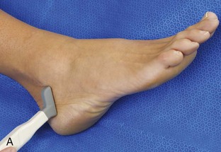
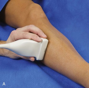
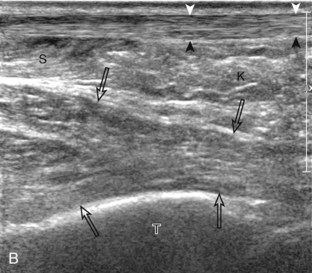
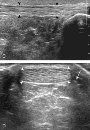
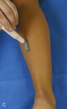
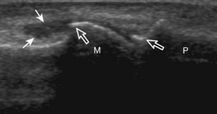
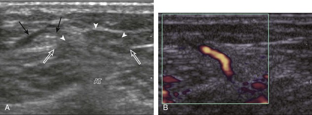
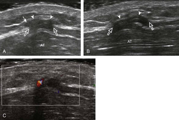
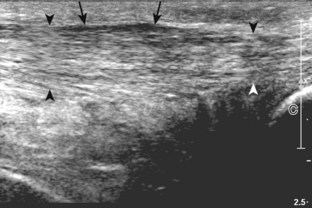
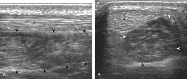
If the patient has no symptoms posteriorly and one wants simply to screen the distal Achilles tendon and plantar aponeurosis for abnormalities, the patient can externally rotate the leg while supine to gain limited access to the posterior ankle. However, for a thorough examination, the patient should lie prone for complete access to the calf and posterior ankle. Dorsiflexion of the ankle elongates the Achilles tendon and reduces anisotropy. The Achilles tendon is easily evaluated because the transducer is placed in the sagittal plane long axis to the tendon fibers from a posterior approach (Fig. 8-22A). In long axis, the Achilles tendon should be fairly uniform in thickness (see Fig. 8-22B and C). The transducer is moved superiorly from the distal calf to the calcaneus, and the transducer is turned 90 degrees for evaluation in short axis; in this plane, the anterior margin of the Achilles tendon is predominantly flat or concave and should not be diffusely convex posterior (see Fig. 8-22D). When imaged from superior to inferior in short axis, the Achilles tendon fibers rotate 90 degrees, with the gastrocnemius component lateral and the soleus medial. A thin tendon, the plantaris, can be seen directly medial to the Achilles tendon (see Fig. 8-22D) but is often best appreciated in the setting of an Achilles tendon tear. The plantaris tendon may be absent in up to 20% of individuals.7 Anterior to the Achilles tendon is a somewhat heterogeneous fat pad called Kager fat pad. Distally, a small amount of anechoic fluid (up to 2.5 mm anteroposterior) can be seen in the retrocalcaneal bursa.12 In evaluation of the retro-Achilles bursa, located superficial to the distal Achilles tendon, it is important to float the transducer on a layer of thick gel so as not to efface the bursa and displace fluid out of the field of view.
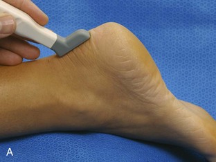
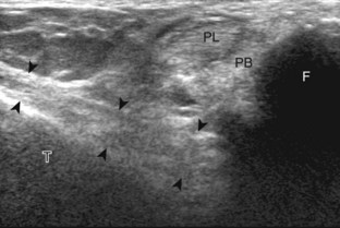
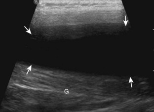
The transducer is then moved over the plantar aspect of the heel to evaluate the plantar aponeurosis (Fig. 8-23A). The transducer is placed in the sagittal plane over the plantar and medial aspect of the heel long axis to the plantar aponeurosis, which appears hyperechoic, uniform, and 4 mm or less in thickness at the calcaneal attachment (see Fig. 8-23B).18 Any identified disorder is also assessed in short axis. More distal assessment of the plantar aponeurosis can be carried out if symptoms or history warrants such evaluation.
Evaluation of the Calf
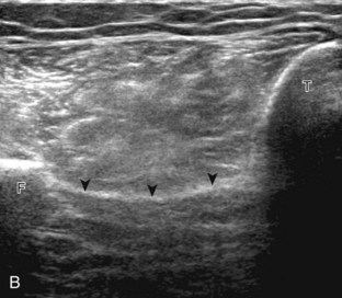
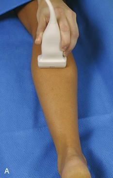
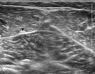
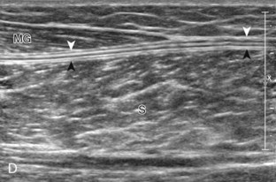
Structures of interest in the posterior calf include the soleus, the medial and lateral heads of the gastrocnemius, and the plantaris. Evaluation begins in the transverse plane over the posterior mid-calf (Fig. 8-24A). At this location, the medial and lateral heads of the gastrocnemius muscle are identified superficial to the larger soleus muscle (see Fig. 8-24B). At this point, the transducer is centered over the medial head of the gastrocnemius and then is moved distally until the muscle tapers. The transducer is then turned 90 degrees to visualize the normal tapering appearance of the medial gastrocnemius head over the soleus in long axis, a very common site of injury (see Fig. 8-24C and D). The lateral head of the gastrocnemius can be evaluated in a similar manner. It is also important to evaluate the entire calf for pathologic processes, although the patient often indicates a site of symptoms to focus evaluation. The thin, hyperechoic plantaris tendon, when present, can be seen in the posterior calf deep to the gastrocnemius muscle.7 Initially, the plantaris crosses midline posterior to the knee joint and then moves medial directly between the muscle bellies of the medial head of the gastrocnemius and soleus muscles. Distally, the medial and lateral heads of the gastrocnemius combine with the soleus to form the Achilles tendon. The plantaris tendon courses along the medial aspect of the Achilles tendon to insert on the calcaneus.
Evaluation of the Forefoot
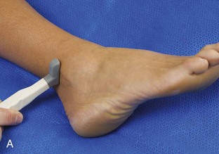
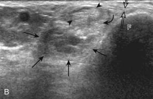
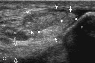
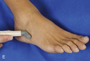
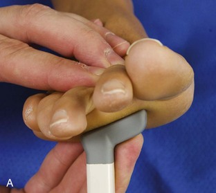
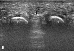
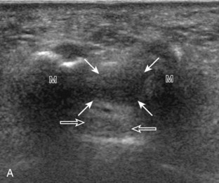
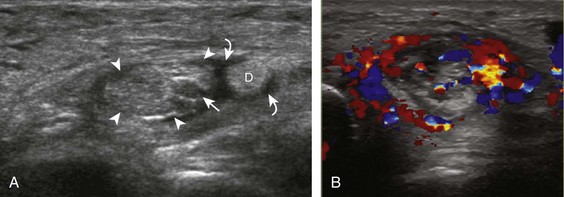
Evaluation of the distal aspect of the foot is largely guided by the patient’s symptoms or history. Tendons around the digits, joint processes, soft tissue fluid collections, and masses can be assessed with ultrasound. If indicated, the forefoot can be assessed for Morton neuroma.19 This is accomplished by placement of the transducer in the coronal plane on the body or short axis to the metatarsals, over the metatarsal heads from a plantar approach (Fig. 8-25A). The examiner’s finger from the other hand is placed at the dorsal aspect of the forefoot over the web space to be evaluated (see Fig. 8-25B). This maneuver assists evaluation because the distal metatarsals are separated and the intermetatarsal space is widened, and it also reproduces the patient’s symptoms when a neuroma is present. Evaluation for Morton neuroma also continues in long axis in the sagittal plane (see Fig. 8-25C). A similar long axis image can be obtained with the transducer over the dorsal foot and manual palpation over the plantar aspect. Resolution is often improved given the thinner dorsal soft tissues compared with the plantar aspect. Returning to the plantar short axis approach, dynamic assessment for Morton neuroma can be completed by manually squeezing the metatarsals together from side to side and imaging from a plantar approach. This maneuver (called the sonographic Mulder sign) will cause plantar displacement of a neuroma also producing symptoms.20 When screening for inflammatory arthritis, in addition to evaluation of a symptomatic region, the fifth metatarsal head and medial first metatarsal head should be routinely imaged to assess for rheumatoid arthritis and gout, respectively.
Joint and Bursal Abnormalities
Joint Effusion and Synovial Hypertrophy
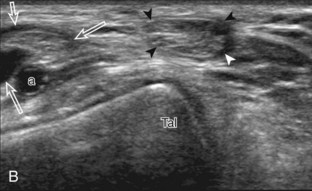
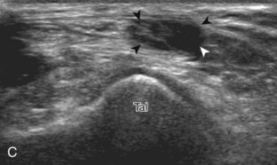
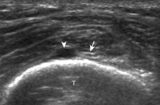
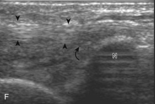
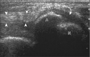
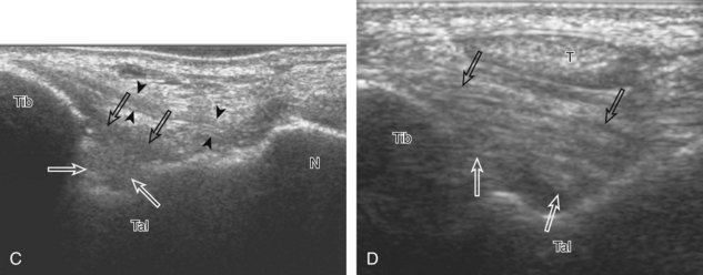
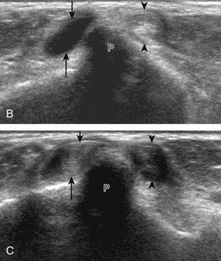
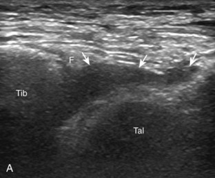
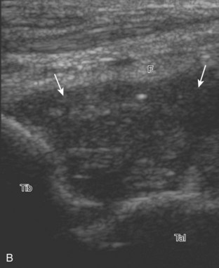
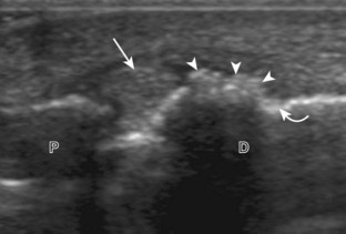
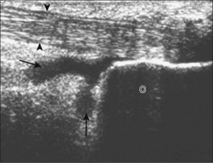
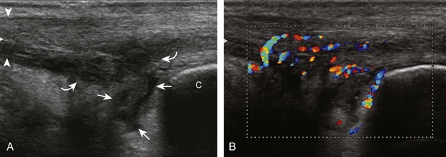
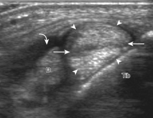
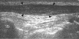
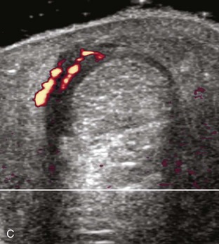
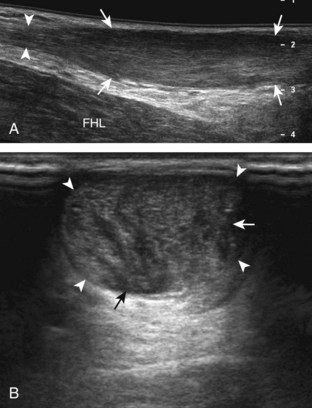
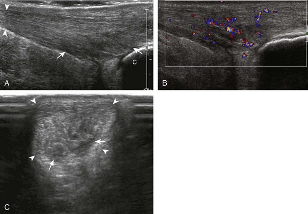
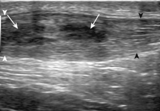
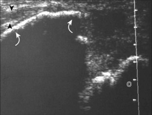
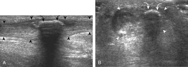
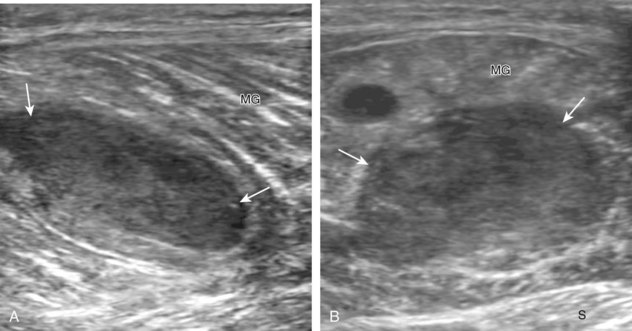
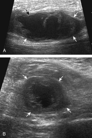
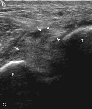
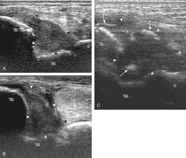
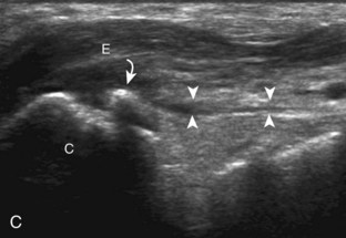
Evaluation for joint pathology should focus on key joint recesses for effusion and synovial hypertrophy. For the ankle or tibiotalar joint, the anterior recess with the foot in slight plantar flexion is the most sensitive position and location to identify joint effusion.21 Simple fluid distention of a joint is typically anechoic. Joint distention is seen in the sagittal plane or in the lateral aspect of the anterior joint recess (Fig. 8-26). A small amount of fluid may be found in the anterior ankle joint recess in normal volunteers; this fluid may measure up to 1.8 mm anteroposterior.12 It is important not to mistake the 1 to 2 mm of hypoechoic hyaline cartilage that covers the talar dome to the talar neck for joint effusion (see Fig. 8-2B). For the foot, dorsal recesses of the tarsal, metatarsophalangeal, and interphalangeal joints are targeted. With regard to the metatarsophalangeal joints, each dorsal joint recess distends proximally over the metatarsal (Fig. 8-27A) as well as over the proximal phalanx when large (see Fig. 8-27B). Causes for anechoic joint effusion are many and include infection (Fig. 8-28), trauma, osteoarthritis (Fig. 8-29), and other arthritides (discussed later). Although commonly seen and asymptomatic, joint fluid within the first metatarsophalangeal joint often relates to early degenerative joint disease because this joint is a common site for osteoarthritis. Intra-articular bodies from degenerative arthritis and trauma appear hyperechoic with possible shadowing within a joint recess (Fig. 8-30). Intra-articular bodies may also migrate to the medial ankle tendon sheaths (see Fig. 8-68B) because communication with the ankle joint is common.
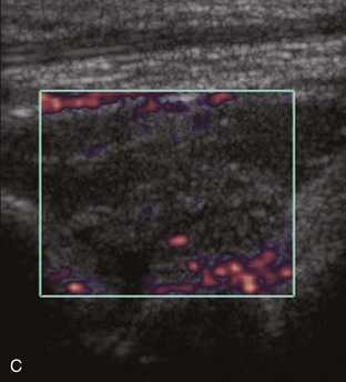
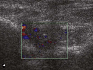
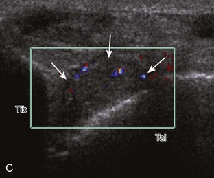
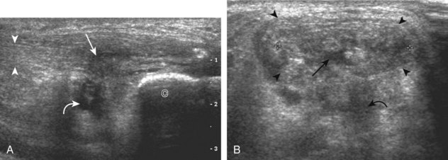
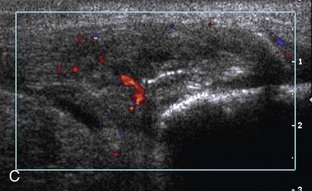
Increased echogenicity of joint fluid can be the result of complex fluid, as seen in infection (Figs. 8-31 and 8-32) and hemorrhage (Fig. 8-33). Echogenic joint fluid may resemble synovial hypertrophy (Figs. 8-34). To assist in this differentiation, compressibility and internal echo movement with transducer pressure, redistribution with joint movement, and lack of flow on color and power Doppler imaging suggest complex fluid rather than synovitis (Videos 8-2 and 8-3) . Echogenicity and vascularity do not predict infection, and ultrasound-guided aspiration should be considered if there is concern for infection. In the setting of synovial hypertrophy, adjacent cortical irregularity may be from erosions, which can be seen in inflammatory (see below for inflammatory arthritis and Chapter 2 for infection) and noninflammatory conditions, which include pigmented villonodular synovitis22 (Fig. 8-35) and synovial (osteo)chondromatosis (Fig. 8-36). In the latter condition, hyperechoic and possibly shadowing foci may be identified.23 Synovial hypertrophy may also be found in the ankle joint deep to the anterior talofibular ligament in anterolateral impingement syndrome (Fig. 8-37), where echogenic synovial hypertrophy greater than 10 mm is associated with symptoms and adjacent ligament abnormality.24 Nonspecific mild synovial thickening, usually with little or no flow on color or power Doppler imaging, can be seen with osteoarthritis and may not correlate with patient symptoms (Fig. 8-38).25,26
Inflammatory Arthritis
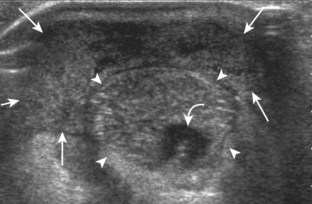
Important target sites for arthritis evaluation in addition to any focal symptomatic area include the distal fifth and first metatarsal heads because these are common sites for involvement from rheumatoid arthritis and gout, respectively. With regard to rheumatoid arthritis, ultrasound findings include joint effusion (Fig. 8-39) and synovial hypertrophy, which is usually hypoechoic (Figs. 8-40 and 8-41) (see Video 8-2), but is possibly isoechoic (Figs. 8-42 and 8-43) (see Video 8-3), compared with subcutaneous fat, with possible increased flow on color or power Doppler imaging.27 In the presence of synovial hypertrophy, disruption of the normally smooth bone cortex in two planes indicates erosions. Because the ultrasound findings of rheumatoid arthritis are not specific and resemble other inflammatory conditions, including other systemic arthritides and infection, the distribution of the findings is very helpful along with radiographic and serologic correlation. The fifth metatarsal head is the most common site of erosions in rheumatoid arthritis (Fig. 8-44) (Video 8-4) , with less common involvement of the other metatarsophalangeal joints and first interphalangeal joint.28–30 It is important not to misinterpret the numerous concavities of the distal metatarsal cortex as an erosion.31 Other manifestations of rheumatoid arthritis in the foot and ankle include the retrocalcaneal bursitis (Fig. 8-45), adventitious bursae (see Fig. 8-61A and Video 8-4), hypoechoic rheumatoid nodules (Fig. 8-46),32 and abnormalities of the tendons and tendon sheath (see Tendon and Muscle Abnormalities).
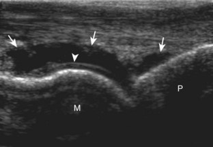
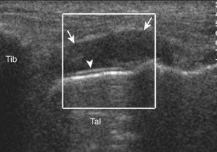
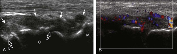
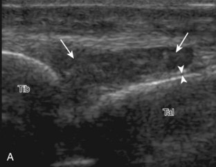
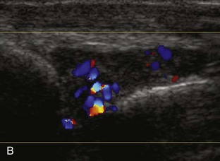
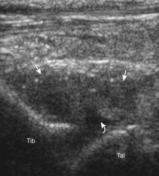
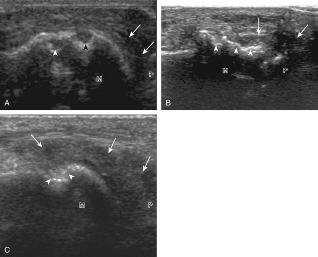
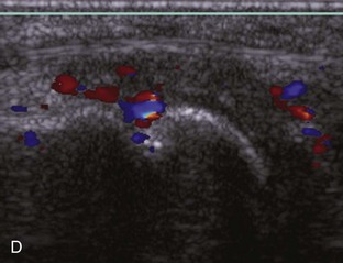
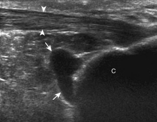
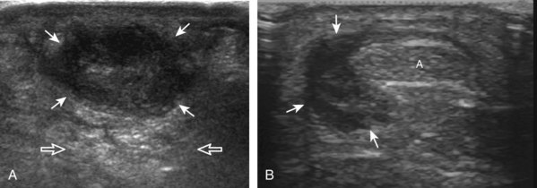
FIGURE 8-46 Rheumatoid arthritis: rheumatoid nodule.
(B, Courtesy of Brian Robertson, Ann Arbor, Mich.)
With regard to gout, the most common site of involvement is the first metatarsophalangeal joint. Within a joint, one may see effusion (Fig. 8-47), synovial hypertrophy (Fig. 8-48), hyperechoic foci (representing microtophi) (Fig. 8-49), echogenic fluid (representing diffuse crystals) (Fig. 8-50), and coating of the hyaline cartilage with monosodium urate crystals (called the double contour sign) (Fig. 8-51).33 The latter finding has been shown to disappear when the serum urate level decreases below 6 mg/dL.34 Imaging at the medial aspect long axis to the distal first metatarsal will show amorphous hyperechoic tophus with anechoic inflammatory halo, with possible direct extension into a cortical erosion (Figs. 8-52 and 8-53) (Video 8-5) .35 Tophi may also involve tendon (Fig. 8-54) and tendon sheaths (Fig. 8-55) (Video 8-6)
  , bursae, and other joints.
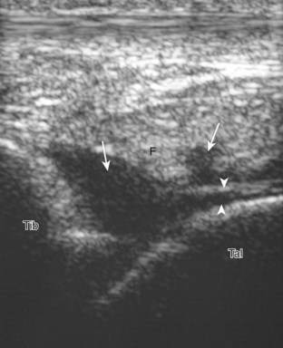
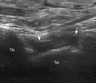
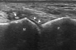
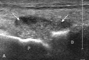
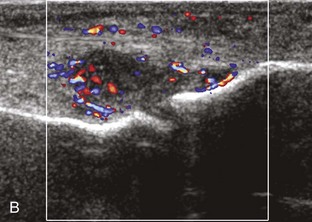
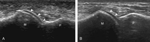
FIGURE 8-51 Gout: urate icing (double contour sign).
(A, Courtesy of Ralf Thiele, MD, Rochester, NY.)
Other inflammatory arthritides include seronegative spondyloarthropathies, such as reactive arthritis and psoriatic arthritis. The ultrasound findings of this category of inflammatory arthritis include nonspecific intra-articular findings of joint fluid, synovial hypertrophy, and possible erosions; however, the finding of bone proliferation in the form of inflammatory enthesopathy at tendon and ligament attachments is characteristic of seronegative spondyloarthropathy (Fig. 8-56).36 Because degenerative enthesopathy is common at several sites in the foot and ankle, such as at the Achilles tendon attachment, correlation with radiography and identifying true inflammatory findings at ultrasound are critical.
Bursal Abnormalities
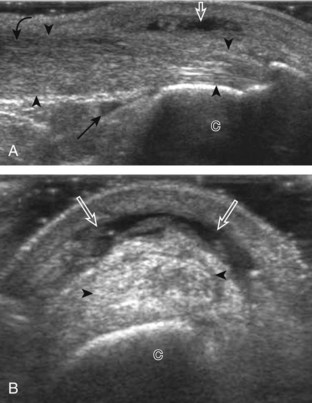
There are two bursae around the distal Achilles tendon: the retrocalcaneal and retro-Achilles bursae. The retrocalcaneal bursa, located between the calcaneus and distal Achilles tendon, may normally contain fluid with anteroposterior distention up to 2.5 mm.12 Abnormal distention of the retrocalcaneal bursa may be mechanical (Fig. 8-57), from adjacent tendon tear (Fig. 8-58), from primary inflammation as in rheumatoid arthritis (see Fig. 8-45), or related to adjacent Achilles enthesopathy. The retro-Achilles bursa, located superficial to the distal Achilles tendon, is not normally visualized and is considered an adventitious bursa. Distention of the retro-Achilles bursa may also be mechanical or inflammatory (Fig. 8-59). The presence of an abnormally distended retrocalcaneal bursa and retro-Achilles bursa with adjacent abnormalities of the Achilles tendon and a prominent posterior superior aspect of the calcaneus is described in patients with Haglund syndrome (Fig. 8-60).37
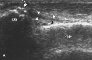
Bursae may also form around the foot and ankle at sites of abnormal pressure, termed adventitious bursae (Fig. 8-61) (Video 8-4).38 Another site of an adventitious bursa is superficial to the medial malleolus (Fig. 8-62).39 Normal bursae are located between the metatarsal heads, called intermetatarsal bursae, and are often distended in associated with Morton neuromas (see Fig. 8-151).40 Another bursa at the anterior ankle that commonly contains minimal fluid is the “bursa sinus tarsi” or “bursa mucosa Gruberi” located between the extensor digitorum longus tendons and the talus (Fig. 8-63).41 Unlike a ganglion cyst, this bursa is easily compressed with transducer pressure and in a characteristic location deep to the extensor digitorum longus (Video 8-7) .
.
Tendon and Muscle Abnormalities
Medial Ankle
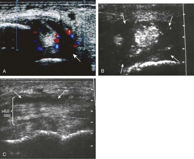
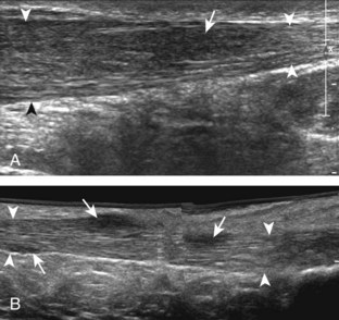
Of the medial tendons, the tibialis posterior tendon is most frequently abnormal, usually at the level of the medial malleolus. Tenosynovitis is characterized by distention of the tendon sheath and may be anechoic if it consists of simple fluid (Fig. 8-64A).42 Tendon sheath distention that is of increased echogenicity may be from complex fluid or synovial hypertrophy; when distention is not anechoic, displacement and internal movement of echoes with transducer pressure as well as absence of internal color flow suggest complex fluid (see Fig. 8-64B).43 Up to 4 mm of fluid may normally distend the posterior tibial tendon sheath just beyond the medial malleolus.12 This normal fluid may be asymmetrical, but a helpful feature is the lack of symptoms with transducer pressure and lack of flow on color Doppler imaging. In addition, the ankle joint can normally communicate with the medial tendon sheaths, especially the flexor hallucis longus tendon. Distention of the posterior tibial tendon sheath greater than 5.8 mm indicates early posterior tibial tendon dysfunction (see Fig. 8-64C).44
Tenosynovitis is commonly mechanical or traumatic, potentially associated with an underlying tendon abnormality. Inflammation related to systemic arthritis, such as seronegative spondyloarthropathy (Fig. 8-65) and rheumatoid arthritis (Fig. 8-66), is another cause. Uncommonly, infection can involve the tendon sheath as an extension from adjacent soft tissue or bone infection (see Fig. 8-64B). Regardless of origin, a peripheral rim of increased flow may be demonstrated on color or power Doppler imaging (see Fig. 8-64A). While more commonly hypoechoic, synovial tissue surrounding a tendon may be isoechoic or hyperechoic to tendon; toggling the transducer when imaging the tendon in short axis will differentiate tendon from echogenic synovial hypertrophy in that the latter does not demonstrate anisotropy and will remain hyperechoic adjacent to the hypoechoic tendon (Fig. 8-67). Tendon sheath distention may also focally involve the flexor hallucis longus tendon at the level of the os trigonum, posterior to the talus in the setting of os trigonum syndrome. More distally, tendon sheath distention may also occur where the flexor hallucis longus and flexor digitorum longus tendons cross (the knot of Henry) under the mid-foot (Fig. 8-68A). Because of the normal communication between the medial tendon sheaths and the ankle joint, intra-articular bodies may migrate into a medial tendon sheath (see Fig. 8-68B). Marked focal distention of a single tendon sheath in the absence of anterior ankle joint recess distention suggests tenosynovitis, rather than communicating ankle joint fluid (Fig. 8-69).
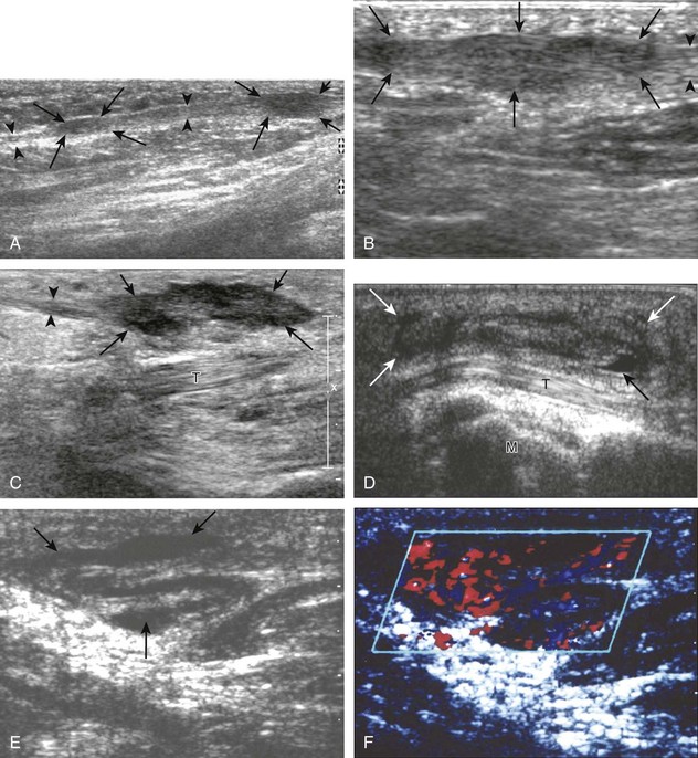
Tendinosis is characterized by hypoechoic enlargement of the involved tendon, without disruption of tendon fibers (Fig. 8-70).45 The involved tendon appears hypoechoic and swollen. The term tendinosis is used rather than tendinitis because this condition typically represents a degenerative process and not an inflammatory process. Tendinosis commonly involves a segment of tendon that courses around an osseous structure, such as at the medial malleolus.
Partial-thickness tears may initially occur as well-defined intrasubstance anechoic or hypoechoic areas or clefts that partially disrupt the tendon fibers, often in the setting of underlying tendinosis (Fig. 8-71).46 It is difficult to differentiate between severe intrasubstance tendinosis and interstitial tear in the continuum of a diseased tendon, although the latter is more likely if the abnormality is well defined and anechoic. One type of tear is a longitudinal split, which may extend to one (Fig. 8-72) or two (Fig. 8-73) tendon surfaces.47 This latter type of tear is best visualized with the tendon in short axis, where the normal tendon is split into two bundles separated by anechoic or hypoechoic fluid, hemorrhage, or synovial hypertrophy. A longitudinal split of the tibialis posterior tendon may be associated with abnormal tendon dislocation or subluxation, which may be apparent only during ankle movement (Fig. 8-74).48 Direct visualization with ultrasound is important during a dynamic maneuver because tendon subluxation may be transient. An avulsed bone fragment from the medial margin of the medial malleolus at the attachment of the flexor retinaculum increases the risk for tibialis posterior dislocation (see Fig. 8-74). Partial-thickness tendon tears may also occur from abnormal contact between a tendon and fixation hardware (Fig. 8-75), between a tendon and a fracture fragment (Fig. 8-76), or when entrapped within a fracture (Fig. 8-77).49
Full-thickness complete tears are characterized by full-width fiber disruption, tendon stump retraction, and interposed fluid, hemorrhage, or synovial hypertrophy that fills the torn tendon gap (Fig. 8-78).47 Tear of the tibialis posterior tendon may occur at the level of the medial malleolus. In short axis, it is important not to mistake the intact flexor digitorum longus tendon for the tibialis posterior tendon when the latter is torn and retracted from view. The tibialis posterior tendon may also tear distally or avulse a fragment of the navicular bone, especially in diabetic patients, associated with tendon retraction. More commonly, a bone in the distal tibialis posterior tendon represents an accessory navicular, which is a normal variant that may become symptomatic in some individuals when the synchondrosis between the accessory navicular and the native navicular is injured (Fig. 8-79). Pain induced by focal pressure from the transducer over the bone fragment is a helpful finding. The flexor digitorum longus tendon may be rerouted to the navicular for treatment of a complete tibialis posterior tendon tear. Ultrasound can evaluate for associated complications, such as flexor digitorum longus tendon avulsion from the implantation site on the navicular (Fig. 8-80).
Disorders of the other medial tendons are less common. Nonetheless, it is important to evaluate the flexor digitorum longus and flexor hallucis longus tendons, at least at locations where pathology may occur, such as at the medial malleolus and posterior malleolus, respectively. This approach ensures a thorough evaluation, which is important when patient symptoms are referred from adjacent structures or locations. Patient history and symptoms may be used to guide evaluation to ensure that pathologic features are not overlooked. Evaluation for tibialis posterior tendon dysfunction should also include the adjacent spring ligament for abnormalities.46 It is also important always to consider dynamic imaging of tendons. In addition to posterior tibial tendon dislocation (see Fig. 8-74B), another example of this application is dynamic evaluation of the flexor hallucis longus tendon to diagnose impingement (Fig. 8-81) (Video 8-8) .
.
Lateral Ankle
As in the medial tendons, tenosynovitis of the peroneal tendons may occur at the level of the lateral malleolus, which appears anechoic from simple fluid, or hypoechoic, isoechoic, or hyperechoic from complex fluid or synovial hypertrophy (Fig. 8-82).50 Although less common than the medial tendon sheaths, up to 3.1 mm of fluid may normally distend the peroneal tendon sheaths, usually just distal to the lateral malleolus.12 Synovial tissue, although more commonly hypoechoic, may also appear isoechoic or hyperechoic relative to subcutaneous fat, which may simulate tendon (see later). The presence of hyperemia on color or power Doppler imaging suggests that hypoechoic distention is from synovial hypertrophy, rather than from complex fluid.43
Tendinosis is also common at the lateral malleolus, where it appears as hypoechoic enlargement of the involved tendon without tendon fiber disruption (Fig. 8-83).51 Well-defined abnormalities within the substance of the tendon could represent severe tendinosis (Fig. 8-84) or an intrasubstance tendon tear (Fig. 8-85). An abnormal hypoechoic or anechoic cleft that extends to the tendon surface is characteristic of a longitudinal split (Figs. 8-86 and 8-87).52 In the diagnosis of peroneal tendon tear, ultrasound has been shown to be 100% sensitive and 90% accurate.51 Although involvement of either peroneal tendon is possible, the peroneus brevis tendon is more commonly torn, in part because of its more common location between the peroneus longus and fibula. Initially, the peroneus brevis tendon appears as a horseshoe shape that encompasses the peroneus longus tendon with a small cleft.51 The two segments of peroneus brevis tendon may separate, best appreciated in short axis, and the peroneus longus tendon may be seen to interpose between the two peroneus brevis tendon pieces (Video 8-9) .51
.51
At its attachment on the fibula, the superior peroneal retinaculum may be injured, which may appear as hypoechoic thickening or complete disruption with associated cortical irregularity (Fig. 8-88).53 With complete retinaculum discontinuity, subluxation or dislocation of the peroneal tendons may occur, predisposing to tenosynovitis and tendon tear. Because tendon displacement may only occur transiently, dynamic ankle evaluation with dorsiflexion and eversion is important in this setting for diagnosis of tendon displacement.52,54 With peroneal tendon displacement, the superior peroneal retinaculum may be thickened and partially stripped away from the fibula, termed a type 1 injury (Fig. 8-89A) (Video 8-10) .5 With peroneal tendon subluxation or dislocation, the retinaculum may be detached, without (see Fig. 8-89B) (Video 8-11)
 or with (see Fig. 8-89C and D) (Video 8-12)
 a fibular avulsion bone fragment.5 Peroneal tendon displacement may be transient, so continual observation with sonography is important throughout the dynamic maneuvers (see Fig. 8-89C and D). Intrasheath peroneal tendon subluxation may also be demonstrated dynamically, which is associated with an abnormal convex posterior contour of the posterior fibula, low-lying peroneus brevis muscle, peroneus quartus, and subsequent tendon tear (Fig. 8-90) (Videos 8-13 to 8-15)
 .54,55 Less commonly, tendon subluxation may occur at the level of the peroneal tubercle. Even in the absence of abnormal subluxation, an enlarged or hypertrophied peroneal tubercle may be associated with peroneal tendon pathology (Fig. 8-91).56 The presence of a low-lying muscle belly of the peroneus brevis may predispose to peroneus tendon pathology, which is diagnosed when the peroneus brevis muscle tissue is identified beyond the fibula (Fig. 8-92).4
It is also important to distinguish an accessory tendon, the peroneus quartus, from a peroneal longitudinal split (Fig. 8-93).6 If unrecognized, the accessory tendon can be misinterpreted as one of the segments of a peroneal tendon split. To differentiate between the two conditions, distal imaging is helpful because a peroneus quartus typically inserts onto the retrotrochlear eminence of the calcaneus, whereas a true longitudinal split follows the direction of the peroneal tendons, and the two tendon pieces eventually reunite to constitute a normal peroneal tendon distally. The peroneus quartus is present in up to 22% of ankles and has a variable appearance representing hypoechoic muscle, hyperechoic tendon, or both.6 It is also important not to misinterpret echogenic synovial tissue near a tendon as a separate segment of tendon, which would falsely indicate a longitudinal split. Toggling the transducer (see Fig. 1-3) causes the tendon tissue to become hypoechoic from anisotropy, whereas echogenic synovial tissue remains hyperechoic (Fig. 8-94).
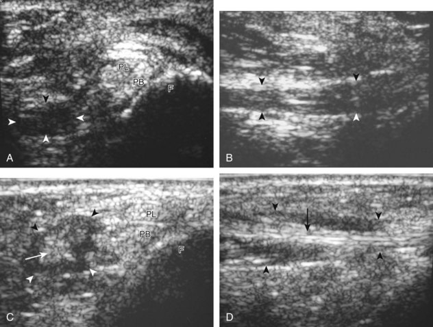
FIGURE 8-93 Peroneus quartus.
(From Chepuri NB, Jacobson JA, Fessell DP, Hayes CW: Sonographic appearance of the peroneus quartus muscle: correlation with MR imaging appearance in seven patients. Radiology 218:415-419, 2001.)
Full-thickness complete tears are characterized by full-width tendon fiber disruption, tendon stump retraction, and interposed hemorrhage or fluid in the torn tendon gap.51 Such tears may occur at the level of the lateral malleolus (Fig. 8-95). More distally, a peroneus longus tendon tear may be associated with fracture of the os peroneum, a normal ossicle within the peroneus longus tendon at the level of the cuboid bone (Fig. 8-96).14 Because the normal os peroneum may be bipartite, it is important to correlate with symptoms elicited by transducer pressure and degree of retraction of the fractured bone fragments, if present. Os peroneum fragment separation of 6 mm or more suggests os peroneum fracture and a full-thickness peroneus longus tendon tear.14 It is important to identify the distal stump of the torn peroneus longus tendon and the proximal os peroneum fragment because retraction to the level of the tibiotalar may be seen (see Fig. 8-96C). Avulsion fracture of the base of the fifth metatarsal may also be seen related to plantar aponeurosis and the peroneus brevis tendon (Fig. 8-97).57
After injury to the lateral ligaments of the ankle, the peroneal tendons may be used in lateral ligament reconstruction.58 In general, the peroneus brevis tendon may be rerouted through a tunnel in the fibula and reattached to the fifth metatarsal, the peroneal brevis tendon may be split so that one segment is looped around the fibula and reattached to itself, or the peroneus brevis may be transected above the fibula and used through various tunnels in the fibula and calcaneus while still attached to the fifth metatarsal.58 At ultrasound, the peroneus brevis split segment may be followed from distal to proximal as it enters into the anterior aspect of the fibula, exits the fibula posteriorly, and then is reattached to itself (Fig. 8-98). It is often helpful to evaluate the peroneus brevis from both the superior aspect and the distal attachment on the fifth metatarsal base to understand which procedure was used, although there are many modifications for each type of reconstruction.
Anterior Ankle and Anterior Lower Leg
Pathology of the anterior tendons is less common than of other areas of the ankle, but similar findings of tenosynovitis (Fig. 8-99), tendinosis (Fig. 8-100), and tendon tear may occur (Fig. 8-101). As a possible variation of normal, the distal tibialis anterior tendon may have a longitudinal split near its insertion.59 Findings that suggest a tendon tear rather than normal variation include associated symptoms, pain with transducer pressure, and associated findings such as hyperemia on color Doppler imaging. Most tibialis anterior tendon tears occur within 3.5 cm of its insertion.59 Full-thickness tibialis anterior tendon tears may retract significantly and produce a mass-like area at the tendon stump possibly associated with an avulsion fracture fragment. Other avulsion fractures may occur, such as extensor digitorum brevis avulsion from the calcaneus (see Fig. 8-101C). Tendon abnormalities may also result from abnormal contact between a tendon and fixation hardware (Fig. 8-102) (Video 8-16) .49 An injured superior extensor retinaculum will appear hypoechoic and thickened (Fig. 8-103).53
Other types of anterior compartment disorders include muscle hernias, which most commonly involve the tibialis anterior, although other muscle compartments may be involved (Fig. 8-104). At ultrasound, a muscle hernia is characterized by muscle tissue that extends superficial to and beyond the enveloping fascial layer (Fig. 8-105).60 A well-defined defect in the thin hyperechoic fascia may be seen, usually at the site of a perforating vessel. A muscle hernia may also occur at a site of intact but thinned fascia.60 Dynamic imaging with joint movement or muscle contraction may be needed to demonstrate the muscle hernia, which may be transient and absent at rest (Videos 8-17 to 8-19) .60,61
Posterior Ankle
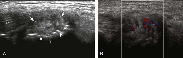
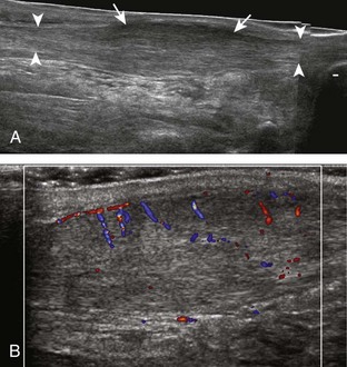
Abnormalities of the Achilles tendon may involve the tendon itself or surrounding tissues. Because the Achilles tendon does not possess a true tendon sheath but rather a peritenon, abnormal hypoechoic swelling or anechoic fluid immediately adjacent to the tendon represents paratendinitis (or paratenonitis) (Figs. 8-106 and 8-107).62 Tendinosis, a degenerative process, appears as hypoechoic fusiform swelling of the Achilles tendon but without disruption of the tendon fibers (Figs. 8-108 to 8-111). Achilles tendon abnormalities such as tendinosis may demonstrate increased flow on color or power Doppler imaging (Video 8-20) . Not present in normal Achilles tendons, increased blood flow has been shown to represent neovascularity and not inflammation, which correlates with patient symptoms.63 Power Doppler imaging demonstrates more flow than conventional color Doppler imaging, which originates from the deep or anterior surface of the tendon.63 It is important to float the transducer on a layer of thick gel in evaluation for flow on color or power Doppler imaging. The slightest amount of pressure from the transducer may obliterate visible flow in the Achilles tendon and surrounding soft tissues (Video 8-21)
 . In addition, dorsiflexion at the foot may also obliterate visible blood flow as the Achilles tendon is stretched. When enthesophytes are identified at the distal Achilles tendon, common degenerative enthesopathy should not be confused with inflammatory enthesopathy, the latter of which will show hyperemia, adjacent tendon abnormality, possible erosions, and ill-defined enthesophyte borders at ultrasound and radiography.64,65 The term tendinosis is used rather than tendinitis because no true inflammation is present.66 Tendinosis may be somewhat focal within a tendon segment or may diffusely involve the tendon diameter.66
Partial-thickness Achilles tendon tears may initially appear as a more defined hypoechoic or anechoic area or cleft within the tendon that partially disrupts tendon fibers (Fig. 8-112); Achilles tendon enlargement greater than 1 cm and significant intrinsic tendon abnormalities indicate a partial-thickness tear.66 Partial-thickness tears can extend to the surface of the Achilles tendon and usually are associated with tendinosis. The use of dynamic imaging by flexing the ankle is important to demonstrate tendon fiber continuity to exclude full-thickness tendon tear (Video 8-22) . Achilles tendinosis and partial-thickness tears may also involve the extreme distal aspect of the Achilles tendon, often associated with cortical irregularity of the calcaneus and adjacent retrocalcaneal or retro-Achilles bursal fluid (Fig. 8-113). The combination of a distal Achilles tendon abnormality, adjacent bursal distention (retrocalcaneal and retro-Achilles), and prominence of the posterosuperior corner of the calcaneus is termed Haglund syndrome (see Fig. 8-60).37
Full-thickness tears of the Achilles tendon are characterized by complete tendon fiber disruption and tendon retraction, commonly 2 to 6 cm proximal to the calcaneal attachment (Fig. 8-114).67 At the torn tendon ends, the Achilles tendon ends are tapered, and often there is posterior acoustic shadowing from refraction at the tendon stumps (see Fig. 8-114C).67 It is important to increase the depth of field to appreciate the posterior acoustic shadowing, which often assists in localization of the tendon ends for accurate measurements (see Fig. 8-114D). The distal tendon stump commonly is angled anterior toward the Kager fat pad. The torn tendon gap may fill with mixed echogenicity fluid or hemorrhage, or possibly a portion of the adjacent hyperechoic fat pad.68 One important pitfall in the setting of a full-thickness Achilles tendon tear is the presence of an intact plantaris tendon at the medial aspect of the Achilles tendon that may simulate intact Achilles tendon fibers (Fig. 8-115) (Video 8-23) .67 The plantaris tendon is often intact in the setting of a full-thickness Achilles tendon tear, which may be related to the fact that the plantaris is a stronger tendon than the Achilles.69 With a suspected full-thickness Achilles tendon tear, it is always important to consider dynamic imaging to ensure an accurate diagnosis. With passive movement of the foot, tendon retraction at the tear becomes more obvious because one tendon stump moves without translation of movement to the other tendon stump (Fig. 8-116) (Videos 8-24 and 8-25)
 . This becomes important in the setting of a subacute or chronic tendon tear, in which hemorrhage and scar tissue may simulate tendon fibers, and, in fact, partial healing may be present (Video 8-26)
 . If conservative management of a full-thickness Achilles tendon is being considered, the distance of residual distraction at the tendon stumps in neutral and plantar flexion is important information that may change management decisions. After surgical repair, the intact Achilles tendon may be heterogeneous and hypoechoic with hyperechoic suture material, although tendon fiber continuity should be seen (Fig. 8-117) (Video 8-27)
 . A full-thickness recurrent tear of the Achilles tendon repair typically shows tendon retraction (Fig. 8-118). The flexor hallucis longus may also insert into the calcaneus as a treatment for Achilles tendon tear (Fig. 8-119).70 In the diabetic patient, the distal Achilles tendon may avulse a large bone fragment from the calcaneus (Fig. 8-120, online).
Other Achilles tendon abnormalities include ossification of the Achilles tendon, associated with prior trauma, surgery, and ankle immobilization (Fig. 8-121).71 Ultrasound can also identify xanthoma deposition in the Achilles tendon, which represents xanthoma cells, extracellular cholesterol, giant cells, and inflammatory cells, seen in heterozygous familial hypercholesterolemia.72 Such deposits range from focal hypoechoic nodules to a heterogeneously hypoechoic swollen Achilles tendon (Fig. 8-122).73
Calf
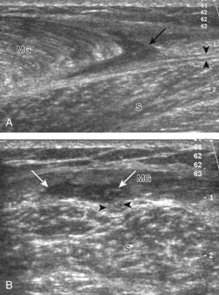
Proximal to the Achilles tendon, the calf muscles and tendons may be injured. One of the most commonly injured structures is the medial head of the gastrocnemius where it tapers distally over the soleus, also called tennis leg (Fig. 8-123).7 At this site, the tendon fibers are disrupted at the aponeurosis with anechoic or hypoechoic fluid or hemorrhage with variable degrees of tendon retraction (Fig. 8-124).74 The patient can usually indicate the site of injury based on the location of symptoms. A remote injury at this site will show increased echogenicity and distortion of the normal fiber architecture (Fig. 8-125).75
Another calf abnormality is a plantaris tendon injury.76,77 A partial-thickness tear appears as a hypoechoic and irregular but intact tendon (Fig. 8-126). A complete tear will appear as a tubular anechoic or mixed-echogenicity fluid collection between the muscle bellies of the medial gastrocnemius and soleus with lack of visualization of the plantaris tendon or tendon discontinuity (Fig. 8-127).76,78 These findings are commonly located more proximally in the calf compared with a medial head of the gastrocnemius tear. Distal medial head of the gastrocnemius and plantaris tears may occur together.
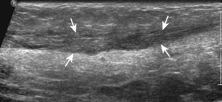
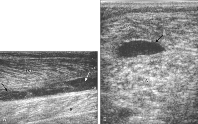
FIGURE 8-127 Plantaris tear.
(From Jamadar DA, Jacobson JA, Theisen SE, et al: Sonography of the painful calf: differential considerations. AJR Am J Roentgenol 179:709-716, 2002.)
Injuries to the soleus and lateral gastrocnemius muscles may occur less commonly, often the result of a direct injury (Fig. 8-128). Although a hematoma may occur in this setting or in patients predisposed to bleeding, the finding of a hematoma, especially if spontaneous, should raise concern for underlying primary malignancy or metastasis as a cause for the hemorrhage (Fig. 8-129). As a normal variation, an accessory soleus muscle can be identified adjacent to the Achilles tendon in the Kager fat pad, which inserts either on the Achilles or onto the calcaneus (Fig. 8-130). Although this may present clinically as a mass, its normal muscle echotexture at sonography and characteristic location are diagnostic for accessory soleus muscle.79 Injury to an accessory soleus may also occur (Fig. 8-131). The calf is a site for cosmetic surgery, where silicone implant is placed superficial to the gastrocnemius muscle for calf augmentation (Fig. 8-132).
Plantar Foot
Abnormalities of the plantar aponeurosis may take several forms.80 A common abnormality represents hypoechoic thickening (>4 mm) of the proximal plantar fascia at the calcaneal origin, best measured in long axis (Fig. 8-133).18,81 Although termed plantar fasciitis, findings may relate to repetitive microtrauma, repair of microtears, degeneration, or edema.18 An acute injury of the plantar fascia may cause hypoechoic thickening if partially torn (Fig. 8-134) or complete disruption with heterogeneous hemorrhage if a full-thickness tear.
Another abnormality that involves the plantar fascia at the central and medial aspect of the foot arch is plantar fibromatosis.82 This condition represents fibroblastic proliferation, commonly at multiple sites in the plantar fascia and bilateral. At ultrasound, plantar fibromatosis appears as hypoechoic or isoechoic fusiform nodules or masses that cause thickening of the plantar fascia and may extend in a dorsal or plantar direction from the plantar fascia (Fig. 8-135) (Video 8-28) .83,84 These nodules may show significant vascularity and increased through-transmission.82 Because the appearance of plantar fibromatosis is not specific for one diagnosis at ultrasound, the location of the abnormality and its multiplicity or bilaterality (if present) suggest the diagnosis of plantar fibromatosis.
Ligament Abnormalities
The lateral ankle is a common site for ligament injury. At ultrasound, partial ligament tears are characterized by hypoechoic thickening of the involved ligament, but some continuous ligament fibers are still seen.85 An acute full-thickness ligament tear is characterized by discontinuity or nonvisualization of the ligament and replacement with hypoechoic or heterogeneous tissue that represents the torn ligament and hemorrhage.85 Osseous avulsions appear as hyperechoic and shadowing bone fragments attached to the involved ligament. Depending on the severity of the ligament tear, remote evaluation of the ligament may show nonvisualization or a thickened ligament. Bone fragments may persist, but lack of pain with transducer pressure is a helpful indicator that the injury was remote.
Of the lateral ankle ligaments, the anterior talofibular ligament is most commonly torn, isolated or in combination with calcaneofibular ligament tear (in up to 70%).85 Isolated tears of the calcaneofibular ligament are not common, whereas posterior talofibular ligament tears are rare.85 Ultrasound has been shown to be effective in evaluation for anterior talofibular ligament tears (Fig. 8-136).86 Dynamic imaging that elicits an anterior drawer sign is helpful in equivocal cases.87 This can be accomplished with the patient lying prone, placing the transducer long axis to the anterior talofibular ligament, and then manually applying anterior directed stress over the heel and observing asymmetrical anterior translation of the talus relative to the fibula. A calcaneofibular ligament tear may appear as abnormal hypoechoic swelling deep to the peroneal tendons at the calcaneus (Fig. 8-137). Lateral ankle ligament reconstruction may involve a direct ligament repair (Fig. 8-138) or the peroneus brevis tendon (see Fig. 8-98).58
Another important lateral ankle ligament is the anterior inferior tibiofibular ligament. Injury to this ligament resembles other ligament injuries (Fig. 8-139).85 Dynamic imaging with the foot in dorsiflexion and eversion will often show widening between the distal tibia and fibula at the site of the ligament tear.88 In the setting of an anterior inferior tibiofibular ligament tear, it is important to consider a possible associated tear of the ankle syndesmosis and interosseous membrane between the tibia and fibula (Fig. 8-140).17 Also termed a high ankle sprain, this injury is associated with prolonged morbidity if it is not accurately diagnosed and treated. The superiorly transmitted force of a high ankle sprain not only may propagate through the interosseous membrane but also may exit as a high fibular fracture, which is termed a Maisonneuve fracture (see Fig. 8-140B). The fibular fracture appears as a cortical step-off at ultrasound. This type of injury may also be associated with an isolated posterior malleolus fracture of the tibia.
Deltoid ligament tears are more difficult to diagnose at ultrasound, largely because this structure represents the confluence of several ligaments, unlike the single defined ligaments laterally.8 Although each of the individual components of the deltoid ligament can be evaluated in the normal ankle, deltoid ligament injuries typically produce hypoechoic swelling that involves several components with possible ligament disruption. At ultrasound, there is diffuse hypoechoic swelling or discontinuity of the deltoid ligament with possible hyperechoic avulsion fracture fragments (Fig. 8-141).85,89 Pain with transducer pressure directly over the deltoid ligament is further evidence to support acute injury. The spring ligament may also be injured, which can appear as hypoechoic thickening of the superomedial calcaneonavicular ligament, often associated with adjacent tibialis posterior tendon abnormality (Fig. 8-142).13
Other ligament injuries around the foot and ankle are often manifested by bone avulsion fragments or malalignment of the osseous structures. Although these smaller and less commonly injured ligaments are not routinely evaluated with ultrasound, a patient may direct examination to an area of ligament injury based on symptoms. Examples include avulsion at the calcaneocuboid ligament, the talonavicular ligament, and bifurcate ligament attachment on the anterior process of the calcaneus, which should not be confused with extensor digitorum brevis avulsion (Fig. 8-143).90 In addition, abnormal widening and hypoechoic hemorrhage between the medial cuneiform and second metatarsal base can indirectly suggest Lisfranc ligament disruption (Fig. 8-144).91 Tear of the dorsal tarsometatarsal ligament between the medial cuneiform and second metatarsal base, which can be identified at ultrasound, is another indirect sign of a tear of Lisfranc ligament proper. It is important to not mistake the normal variant os intermetatarsus, located between the first and second metatarsal bases, for a Lisfranc ligament injury–related fracture fragment (Fig. 8-145). Location of the os intermetatarsus distal to the middle cuneiform and normal tarsometatarsal alignment assists in this differentiation.
Fracture
Although it is understood that radiography should be the initial imaging method of choice to evaluate for fracture, it is not uncommon for an radiographically occult fracture to be identified at ultrasound. There are many osseous structures in the ankle and foot, and therefore it is not practical to assess each osseous structure routinely for abnormality. To identify a fracture at ultrasound, one relies on the patient to direct examination based on point tenderness or the focal point of symptoms. It is critical, before completion of an ultrasound examination of the foot or ankle, that the patient be asked to indicate any focal site of symptoms. Identification of a cortical step-off of the normally smooth and echogenic cortical surface is diagnostic for fracture, especially if it is associated with pain from transducer pressure.92 Knowledge of the normal osseous structures and their articulations is essential to not mistake a joint space for a displaced fracture. One may image the normal contralateral foot and ankle for comparison.
Acute fractures may occur at tendon or ligament attachments, and these were discussed earlier, in the tendon and ligament sections of this chapter. Besides these locations, acute fractures may occur essentially anywhere in the foot and ankle, related to the mechanism of injury. For example, distal fibular (Fig. 8-146A) and proximal fifth metatarsal (see Fig. 8-97) fractures are associated with inversion ankle injuries.93 Stress fractures of bone classically involve the metatarsal shafts (Fig. 8-146B and C), the navicular bone (usually in the sagittal plane) (Fig. 8-147A), and the hallux sesamoids (see Fig. 8-147B).94 With stress fractures, early ultrasound findings include focal hypoechogenicity along the cortex from hematoma or periostitis.95 A step-off deformity or fracture line may also be identified. Later with bone remodeling, hyperechoic callous formation becomes evident. Ultrasound can also diagnose physeal injuries in children, which appear as adjacent hypoechoic hemorrhage or edema and possible wide or irregular physis and adjacent subperiosteal hematoma.96 Although difficult to visualize, cortical irregularity and collapse of the metatarsal head (commonly the second) can indicate Freiberg disease or infraction, which is fracture and necrosis of the metatarsal head from repetitive trauma (Fig. 8-148). Ultrasound has been used to assess callous formation after static interlocked nail placement for tibia fracture (Fig. 8-149).94
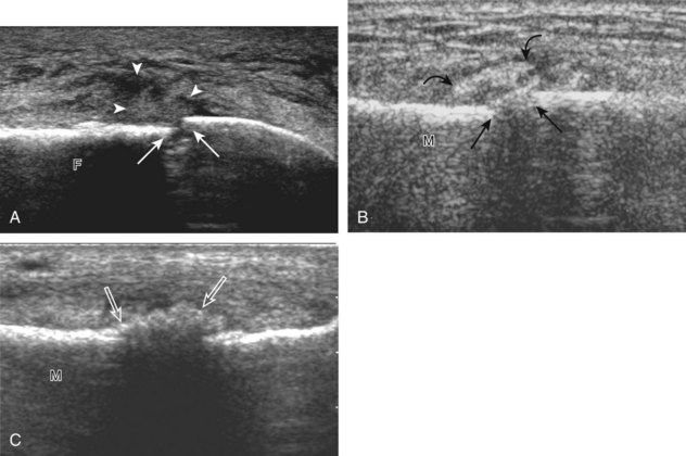
FIGURE 8-146 Fractures: fibula and metatarsal.
(C, From Craig JG, Jacobson JA, Moed BR: Ultrasound of fracture and bone healing. Radiol Clin North Am 37:737-751, ix, 1999.)
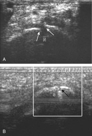
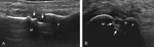
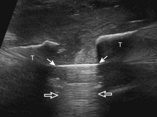
Peripheral Nerve Abnormalities
Morton neuroma is a non-neoplastic enlargement of a common plantar digital nerve as a result of nerve entrapment or trauma characterized by perineural fibrosis, vascular proliferation, endoneurium edema, and axonal degeneration.97 The most common site for Morton neuroma is the third web space, followed by the second, at the level of the metatarsal heads.97 At ultrasound, Morton neuroma appears as a hypoechoic mass, which is more likely symptomatic when it is greater than 5 mm (Fig. 8-150).98 In the coronal plane, the neuroma often extends in a plantar direction from between the metatarsal heads with concave borders medial and lateral.99 In the sagittal plane, identification of the hypoechoic common plantar digital nerve, which enters into the neuroma, ensures the diagnosis (Fig. 8-151).97 This finding, along with noncompressibility of the mass, helps to exclude bursal distention as a cause for a hypoechoic mass (Videos 8-29 and 8-30) . Compression of the neuroma between the transducer at the plantar aspect and the examiner’s finger over the dorsal aspect of the foot should reproduce the patient’s symptoms related to the neuroma. Conversely, if scanning from the dorsal aspect, compression is applied from the plantar aspect. Dynamic evaluation with application of opposed medial and lateral force to compress the metatarsal heads may displace a neuroma in a plantar direction and cause a palpable click (the sonographic Mulder sign), which can increase diagnostic confidence (Fig. 8-152) (Video 8-31)
 .20 This dynamic maneuver can increase sensitivity of ultrasound in diagnosis of an intermetarsal mass from 65% to 100%.100 It is not uncommon for Morton neuromas to be associated with intermetatarsal bursal distention, which can appear as an adjacent anechoic fluid collection or possibly a large complex heterogeneous mass.
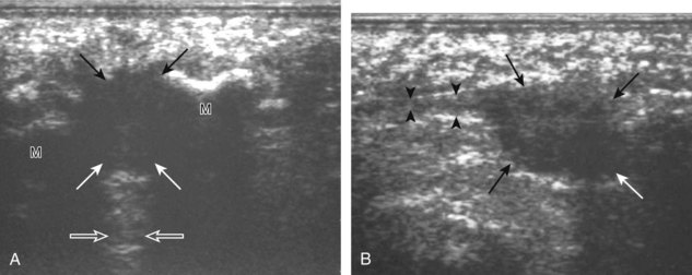
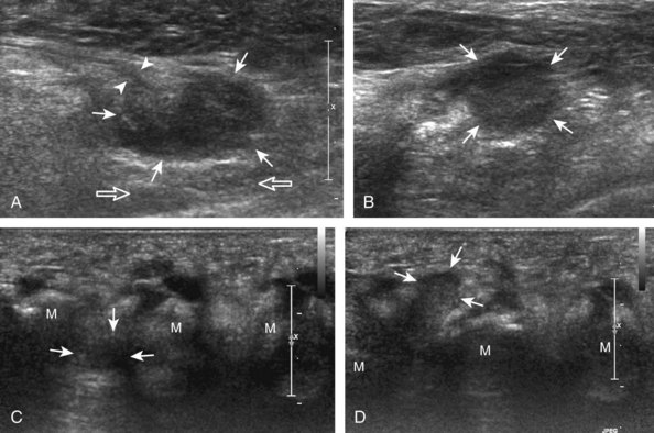
Another example is potential nerve entrapment of the tibial nerve in the tarsal tunnel, which is an enclosed space posterior to the distal tibia bound by the flexor retinaculum that contains the medial tendons and tibial nerve. Tibial nerve entrapment at this site, called tarsal tunnel syndrome, may be secondary to a ganglion cyst (Fig. 8-153) (Video 8-32) , although any space-occupying process can have the same effect.101 Tarsal tunnel syndrome also has been associated with talocalcaneal coalition.101 It is important not to mistake a hypoechoic peripheral nerve sheath tumor, which may be eccentric to the tibial nerve axis and demonstrate increased through-transmission, as a complex ganglion cyst compressing the tibial nerve (Fig. 8-154).102 Another site prone to nerve compression is the superficial peroneal nerve where it pierces the crural fascia at an average of 9 cm proximal to the fibular tip.103 A neuroma can form at this site, appearing swollen and hypoechoic, owing to traction injury, thickened fascia, or muscle hernia (Fig. 8-155) (Video 8-33)
 .104
.104
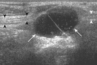
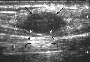
FIGURE 8-154 Schwannoma: tibial nerve.
(From Reynolds DL Jr, Jacobson JA, Inampudi P, et al: Sonographic characteristics of peripheral nerve sheath tumors. AJR Am J Roentgenol 182:741-744, 2004.)
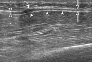
Trauma to a peripheral nerve may cause findings at ultrasound that range from hypoechoic swelling to complete nerve discontinuity with retraction. In the setting of nerve transection, neuroma formation is an expected response as the nerve attempts to regenerate, which appears as hypoechoic swelling of the terminal nerve end (Figs. 8-156 and 8-157).105 Peripheral nerve sheath tumors are discussed in Chapter 2.
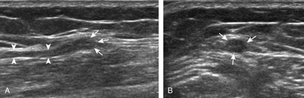
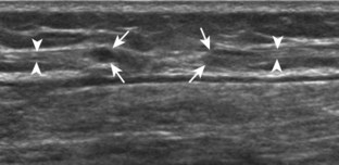
Masses and Cysts
In evaluation of a foot or ankle mass, it is important to determine whether the mass originates from a joint, from the bone, or from the soft tissues apart from a joint. Most joint processes that may manifest as a mass are synovial proliferative disorders, such as pigmented villonodular synovitis (see Fig. 8-35)22 or synovial chondromatosis (see Fig. 8-36). Similarly, a well-defined hypoechoic mass arising from a tendon sheath commonly represents a giant cell tumor of the tendon sheath (pigmented villonodular tenosynovitis) (Fig. 8-158).106 Masses that arise from bone are often malignant or aggressive (see Chapter 2) and are best evaluated with radiography and magnetic resonance imaging. Regarding other soft tissue masses, ultrasound may differentiate cystic and solid masses and may guide percutaneous biopsy or aspiration.
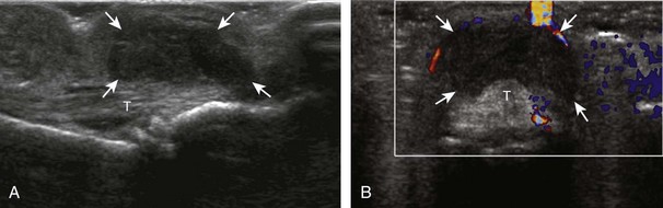
The most common benign mass in the foot and ankle is a ganglion cyst.107 Classically, a ganglion cyst is anechoic, with increased through-transmission and no associated mass (Fig. 8-159A).107 However, many ganglion cysts are hypoechoic, multilocular, and lobular (see Fig. 8-159B and C). In addition, the viscous nature of the fluid may create reflective echoes within the cyst. Location of a ganglion cyst within the tarsal tunnel may compress the tibial nerve (see Fig. 8-153). Ganglion cysts of the foot and ankle may show communication with adjacent joints or tendon sheaths and involve the sinus tarsi (see Fig. 8-159C). It is important not to mistake a bursa, such as the sinus tarsi bursa of Gruberi, between the extensor digitorum longus tendons and talus (see Fig. 8-63) as a ganglion cyst.41 Ultrasound can be used to guide percutaneous aspiration, in which a large-bore needle is often needed because of the high viscosity of the cyst contents. In evaluation of the lateral ankle, it is important not to mistake the normal calcaneofibular ligament in cross section, which may appear hypoechoic as a result of anisotropy, for a small ganglion cyst (see Fig. 8-18C and D).
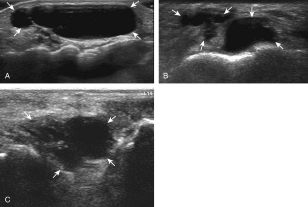
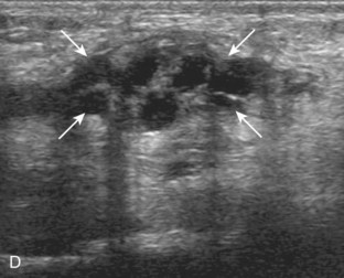
Another type of cyst that may involve the foot is an epidermal inclusion cyst, with implantation of epidermis into the dermis or subcutis from trauma proposed as one cause.108 At ultrasound, an epidermal inclusion cyst typically appears hypoechoic to surrounding tissues but with low-level internal echoes and a hypoechoic rim and increased through-transmission, which at times may simulate a solid mass (Fig. 8-160).109 Increased blood flow on color Doppler imaging and lobulated margins are more likely after cyst rupture.110
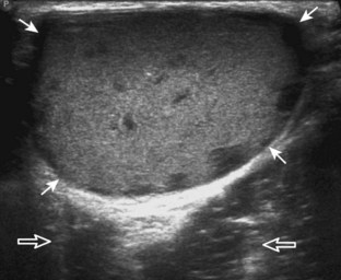
Other benign and malignant masses that are not specific to the foot and ankle are discussed in Chapter 2. Plantar fibromatosis (see Fig. 8-135) was discussed earlier in this chapter. One must also consider the possibility of an inflammatory process that simulates a soft tissue mass, such as a chronic foreign body reaction (see Chapter 2). Other causes for palpable mass include muscle hernia (see Figs. 8-104 and 8-105) and accessory soleus muscle (see Fig. 8-130). Soft tissue masses associated with inflammatory arthritis include rheumatoid nodule (see Fig. 8-46), adventitious bursa (see Fig. 8-61), and gouty tophi (see Fig. 8-55).
1 Lektrakul N, Chung CB, Lai Y, et al. Tarsal sinus: arthrographic, MR imaging, MR arthrographic, and pathologic findings in cadavers and retrospective study data in patients with sinus tarsi syndrome. Radiology. 2001;219:802–810.
2 Louisia S, Masquelet AC. The medial and inferior calcaneal nerves: an anatomic study. Surg Radiol Anat. 1999;21:169–173.
3 Chundru U, Liebeskind A, Seidelmann F, et al. Plantar fasciitis and calcaneal spur formation are associated with abductor digiti minimi atrophy on MRI of the foot. Skeletal Radiol. 2008;37:505–510.
4 Rosenberg ZS, Beltran J, Cheung YY, et al. MR features of longitudinal tears of the peroneus brevis tendon. AJR Am J Roentgenol. 1997;168:141–147.
5 Rosenberg ZS, Bencardino J, Astion D, et al. MRI features of chronic injuries of the superior peroneal retinaculum. AJR Am J Roentgenol. 2003;181:1551–1557.
6 Chepuri NB, Jacobson JA, Fessell DP, et al. Sonographic appearance of the peroneus quartus muscle: correlation with MR imaging appearance in seven patients. Radiology. 2001;218:415–419.
7 Delgado GJ, Chung CB, Lektrakul N, et al. Tennis leg: clinical US study of 141 patients and anatomic investigation of four cadavers with MR imaging and US. Radiology. 2002;224:112–119.
8 Muhle C, Frank LR, Rand T, et al. Collateral ligaments of the ankle: high-resolution MR imaging with a local gradient coil and anatomic correlation in cadavers. Radiographics. 1999;19:673–683.
9 Subhas N, Vinson EN, Cothran RL, et al. MRI appearance of surgically proven abnormal accessory anterior-inferior tibiofibular ligament (Bassett’s ligament). Skeletal Radiol. 2008;37:27–33.
10 Harish S, Jan E, Finlay K, et al. Sonography of the superomedial part of the spring ligament complex of the foot: a study of cadavers and asymptomatic volunteers. Skeletal Radiol. 2007;36:221–228.
11 Castro M, Melao L, Canella C, et al. Lisfranc joint ligamentous complex: MRI with anatomic correlation in cadavers. AJR Am J Roentgenol. 2010;195:W447–455.
12 Nazarian LN, Rawool NM, Martin CE, et al. Synovial fluid in the hindfoot and ankle: detection of amount and distribution with US. Radiology. 1995;197:275–278.
13 Mansour R, Teh J, Sharp RJ, et al. Ultrasound assessment of the spring ligament complex. Eur Radiol. 2008;18:2670–2675.
14 Brigido MK, Fessell DP, Jacobson JA, et al. Radiography and US of os peroneum fractures and associated peroneal tendon injuries: initial experience. Radiology. 2005;237:235–241.
15 Boonthathip M, Chen L, Trudell DJ, et al. Tibiofibular syndesmotic ligaments: MR arthrography in cadavers with anatomic correlation. Radiology. 2010;254:827–836.
16 van den Bekerom MP, Raven EE. The distal fascicle of the anterior inferior tibiofibular ligament as a cause of tibiotalar impingement syndrome: a current concepts review. Knee Surg Sports Traumatol Arthrosc. 2007;15:465–471.
17 Durkee NJ, Jacobson JA, Jamadar DA, et al. Sonographic evaluation of lower extremity interosseous membrane injuries: retrospective review in 3 patients. J Ultrasound Med. 2003;22:1369–1375.
18 Cardinal E, Chhem RK, Beauregard CG, et al. Plantar fasciitis: sonographic evaluation. Radiology. 1996;201:257–259.
19 Lee KS. Musculoskeletal ultrasound: how to evaluate for Morton’s neuroma. AJR Am J Roentgenol. 2009;193:W172.
20 Torriani M, Kattapuram SV. Technical innovation. Dynamic sonography of the forefoot: the sonographic Mulder sign. AJR Am J Roentgenol. 2003;180:1121–1123.
21 Jacobson JA, Andresen R, Jaovisidha S, et al. Detection of ankle effusions: comparison study in cadavers using radiography, sonography, and MR imaging. AJR Am J Roentgenol. 1998;170:1231–1238.
22 Yang PY, Wang CL, Wu CT, et al. Sonography of pigmented villonodular synovitis in the ankle joint. J Clin Ultrasound. 1998;26:166–170.
23 Roberts D, Miller TT, Erlanger SM. Sonographic appearance of primary synovial chondromatosis of the knee. J Ultrasound Med. 2004;23:707–709.
24 McCarthy CL, Wilson DJ, Coltman TP. Anterolateral ankle impingement: findings and diagnostic accuracy with ultrasound imaging. Skeletal Radiol. 2008;37:209–216.
25 Hayashi D, Roemer FW, Katur A, et al. Imaging of synovitis in osteoarthritis: current status and outlook. Semin Arthritis Rheum. 2011;41:116–130.
26 Keen HI, Conaghan PG. Ultrasonography in osteoarthritis. Radiol Clin North Am. 2009;47:581–594.
27 Wakefield RJ, Balint PV, Szkudlarek M, et al. Musculoskeletal ultrasound including definitions for ultrasonographic pathology. J Rheumatol. 2005;32:2485–2487.
28 Riente L, Delle Sedie A, Scire CA, et al. Ultrasound imaging for the rheumatologist. XXXI. Sonographic assessment of the foot in patients with rheumatoid arthritis. Clin Exp Rheumatol. 2011;29:1–5.
29 Sheane BJ, Beddy P, O’Connor M, et al. Targeted ultrasound of the fifth metatarsophalangeal joint in an early inflammatory arthritis cohort. Arthritis Rheum. 2009;61:1004–1008.
30 Lopez-Ben R, Bernreuter WK, Moreland LW, et al. Ultrasound detection of bone erosions in rheumatoid arthritis: a comparison to routine radiographs of the hands and feet. Skeletal Radiol. 2004;33:80–84.
31 Torshizy H, Hughes TH, Trudell D, et al. Anatomic features of metatarsal heads that simulate erosive disease: cadaveric study using CT, radiography, and dissection with special emphasis on cross-sectional characterization of osseous anatomy. AJR Am J Roentgenol. 2008;190:W175–181.
32 Nalbant S, Corominas H, Hsu B, et al. Ultrasonography for assessment of subcutaneous nodules. J Rheumatol. 2003;30:1191–1195.
33 Thiele RG. Role of ultrasound and other advanced imaging in the diagnosis and management of gout. Curr Rheumatol Rep. 2011;13:146–153.
34 Thiele RG, Schlesinger N. Ultrasonography shows disappearance of monosodium urate crystal deposition on hyaline cartilage after sustained normouricemia is achieved. Rheumatol Int. 2010;30:495–503.
35 de Avila Fernandes E, Kubota ES, Sandim GB, et al. Ultrasound features of tophi in chronic tophaceous gout. Skeletal Radiol. 2011;40:309–315.
36 Gutierrez M, Filippucci E, De Angelis R, et al. A sonographic spectrum of psoriatic arthritis: “the five targets. Clin Rheumatol. 2010;29:133–142.
37 Lee JC, Calder JD, Healy JC. Posterior impingement syndromes of the ankle. Semin Musculoskelet Radiol. 2008;12:154–169.
38 Studler U, Mengiardi B, Bode B, et al. Fibrosis and adventitious bursae in plantar fat pad of forefoot: MR imaging findings in asymptomatic volunteers and MR imaging-histologic comparison. Radiology. 2008;246:863–870.
39 Brown RR, Sadka Rosenberg Z, Schweitzer ME, et al. MRI of medial malleolar bursa. AJR Am J Roentgenol. 2005;184:979–983.
40 Zanetti M, Strehle JK, Zollinger H, et al. Morton neuroma and fluid in the intermetatarsal bursae on MR images of 70 asymptomatic volunteers. Radiology. 1997;203:516–520.
41 Lovell AG, Tanner HH. Synovial membranes, with special reference to those related to the tendons of the foot and ankle. J Anat Physiol. 1908;42:415–432.
42 Bianchi S, Poletti PA, Martinoli C, et al. Ultrasound appearance of tendon tears. Part 2: lower extremity and myotendinous tears. Skeletal Radiol. 2006;35:63–77.
43 Breidahl WH, Stafford Johnson DB, Newman JS, et al. Power Doppler sonography in tenosynovitis: significance of the peritendinous hypoechoic rim. J Ultrasound Med. 1998;17:103–107.
44 Chen YJ, Liang SC. Diagnostic efficacy of ultrasonography in stage I posterior tibial tendon dysfunction: sonographic-surgical correlation. J Ultrasound Med. 1997;16:417–423.
45 Premkumar A, Perry MB, Dwyer AJ, et al. Sonography and MR imaging of posterior tibial tendinopathy. AJR Am J Roentgenol. 2002;178:223–232.
46 Kong A, Van Der Vliet A. Imaging of tibialis posterior dysfunction. Br J Radiol. 2008;81:826–836.
47 Miller SD, Van Holsbeeck M, Boruta PM, et al. Ultrasound in the diagnosis of posterior tibial tendon pathology. Foot Ankle Int. 1996;17:555–558.
48 Prato N, Abello E, Martinoli C, et al. Sonography of posterior tibialis tendon dislocation. J Ultrasound Med. 2004;23:701–705.
49 Shetty M, Fessell DP, Femino JE, et al. Sonography of ankle tendon impingement with surgical correlation. AJR Am J Roentgenol. 2002;179:949–953.
50 Bianchi S, Delmi M, Molini L. Ultrasound of peroneal tendons. Semin Musculoskelet Radiol. 2010;14:292–306.
51 Grant TH, Kelikian AS, Jereb SE, et al. Ultrasound diagnosis of peroneal tendon tears: a surgical correlation. J Bone Joint Surg Am. 2005;87:1788–1794.
52 Diaz GC, van Holsbeeck M, Jacobson JA. Longitudinal split of the peroneus longus and peroneus brevis tendons with disruption of the superior peroneal retinaculum. J Ultrasound Med. 1998;17:525–529.
53 Demondion X, Canella C, Moraux A, et al. Retinacular disorders of the ankle and foot. Semin Musculoskelet Radiol. 2010;14:281–291.
54 Neustadter J, Raikin SM, Nazarian LN. Dynamic sonographic evaluation of peroneal tendon subluxation. AJR Am J Roentgenol. 2004;183:985–988.
55 Thomas JL, Lopez-Ben R, Maddox J. A preliminary report on intra-sheath peroneal tendon subluxation: a prospective review of 7 patients with ultrasound verification. J Foot Ankle Surg. 2009;48:323–329.
56 Khoury NJ, el-Khoury GY, Saltzman CL, et al. Peroneus longus and brevis tendon tears: MR imaging evaluation. Radiology. 1996;200:833–841.
57 Theodorou DJ, Theodorou SJ, Kakitsubata Y, et al. Fractures of proximal portion of fifth metatarsal bone: anatomic and imaging evidence of a pathogenesis of avulsion of the plantar aponeurosis and the short peroneal muscle tendon. Radiology. 2003;226:857–865.
58 Chien AJ, Jacobson JA, Jamadar DA, et al. Imaging appearances of lateral ankle ligament reconstruction. Radiographics. 2004;24:999–1008.
59 Mengiardi B, Pfirrmann CW, Vienne P, et al. Anterior tibial tendon abnormalities: MR imaging findings. Radiology. 2005;235:977–984.
60 Beggs I. Sonography of muscle hernias. AJR Am J Roentgenol. 2003;180:395–399.
61 Bianchi S, Abdelwahab IF, Mazzola CG, et al. Sonographic examination of muscle herniation. J Ultrasound Med. 1995;14:357–360.
62 Calleja M, Connell DA. The Achilles tendon. Semin Musculoskelet Radiol. 2010;14:307–322.
63 Richards PJ, Win T, Jones PW. The distribution of microvascular response in Achilles tendonopathy assessed by colour and power Doppler. Skeletal Radiol. 2005;34:336–342.
64 Kiris A, Kaya A, Ozgocmen S, et al. Assessment of enthesitis in ankylosing spondylitis by power Doppler ultrasonography. Skeletal Radiol. 2006;35:522–528.
65 Filippucci E, Aydin SZ, Karadag O, et al. Reliability of high-resolution ultrasonography in the assessment of Achilles tendon enthesopathy in seronegative spondyloarthropathies. Ann Rheum Dis. 2009;68:1850–1855.
66 Astrom M, Gentz CF, Nilsson P, et al. Imaging in chronic Achilles tendinopathy: a comparison of ultrasonography, magnetic resonance imaging and surgical findings in 27 histologically verified cases. Skeletal Radiol. 1996;25:615–620.
67 Hartgerink P, Fessell DP, Jacobson JA, et al. Full- versus partial-thickness Achilles tendon tears: sonographic accuracy and characterization in 26 cases with surgical correlation. Radiology. 2001;220:406–412.
68 Jacobson JA, Miller BS, Morag Y. Golf and racquet sports injuries. Semin Musculoskelet Radiol. 2005;9:346–359.
69 Alfredson H. Midportion Achilles tendinosis and the plantaris tendon. Br J Sports Med. 2011;45:1023–1025.
70 Mahajan RH, Dalal RB. Flexor hallucis longus tendon transfer for reconstruction of chronically ruptured Achilles tendons. J Orthop Surg (Hong Kong). 2009;17:194–198.
71 Richards PJ, Braid JC, Carmont MR, et al. Achilles tendon ossification: pathology, imaging and aetiology. Disabil Rehabil. 2008;30:1651–1665.
72 Bude RO, Adler RS, Bassett DR, et al. Heterozygous familial hypercholesterolemia: detection of xanthomas in the Achilles tendon with US. Radiology. 1993;188:567–571.
73 Bureau NJ, Roederer G. Sonography of Achilles tendon xanthomas in patients with heterozygous familial hypercholesterolemia. AJR Am J Roentgenol. 1998;171:745–749.
74 Bianchi S, Martinoli C, Abdelwahab IF, et al. Sonographic evaluation of tears of the gastrocnemius medial head (“tennis leg”). J Ultrasound Med. 1998;17:157–162.
75 Kwak HS, Han YM, Lee SY, et al. Diagnosis and follow-up US evaluation of ruptures of the medial head of the gastrocnemius (“tennis leg”). Korean J Radiol. 2006;7:193–198.
76 Bianchi S, Sailly M, Molini L. Isolated tear of the plantaris tendon: ultrasound and MRI appearance. Skeletal Radiol. 2011;40:891–895.
77 Leekam RN, Agur AM, McKee NH. Using sonography to diagnose injury of plantaris muscles and tendons. AJR Am J Roentgenol. 1999;172:185–189.
78 Jamadar DA, Jacobson JA, Theisen SE, et al. Sonography of the painful calf: differential considerations. AJR Am J Roentgenol. 2002;179:709–716.
79 Yu JS, Resnick D. MR imaging of the accessory soleus muscle appearance in six patients and a review of the literature. Skeletal Radiol. 1994;23:525–528.
80 McNally EG, Shetty S. Plantar fascia: imaging diagnosis and guided treatment. Semin Musculoskelet Radiol. 2010;14:334–343.
81 Cheng JW, Tsai WC, Yu TY, et al. Reproducibility of sonographic measurement of thickness and echogenicity of the plantar fascia. J Clin Ultrasound. 2012;40:14–19.
82 Griffith JF, Wong TY, Wong SM, et al. Sonography of plantar fibromatosis. AJR Am J Roentgenol. 2002;179:1167–1172.
83 Bedi DG, Davidson DM. Plantar fibromatosis: most common sonographic appearance and variations. J Clin Ultrasound. 2001;29:499–505.
84 Pham H, Fessell DP, Femino JE, et al. Sonography and MR imaging of selected benign masses in the ankle and foot. AJR Am J Roentgenol. 2003;180:99–107.
85 Peetrons P, Creteur V, Bacq C. Sonography of ankle ligaments. J Clin Ultrasound. 2004;32:491–499.
86 Oae K, Takao M, Uchio Y, et al. Evaluation of anterior talofibular ligament injury with stress radiography, ultrasonography and MR imaging. Skeletal Radiol. 2010;39:41–47.
87 Campbell DG, Menz A, Isaacs J. Dynamic ankle ultrasonography: a new imaging technique for acute ankle ligament injuries. Am J Sports Med. 1994;22:855–858.
88 Mei-Dan O, Kots E, Barchilon V, et al. A dynamic ultrasound examination for the diagnosis of ankle syndesmotic injury in professional athletes: a preliminary study. Am J Sports Med. 2009;37:1009–1016.
89 Chen PY, Wang TG, Wang CL. Ultrasonographic examination of the deltoid ligament in bimalleolar equivalent fractures. Foot Ankle Int. 2008;29:883–886.
90 Boutry N, Vanderhofstadt A, Peetrons P. Ultrasonography of anterosuperior calcaneal process fracture: report of 2 cases. J Ultrasound Med. 2006;25:381–385.
91 Woodward S, Jacobson JA, Femino JE, et al. Sonographic evaluation of Lisfranc ligament injuries. J Ultrasound Med. 2009;28:351–357.
92 Wang CL, Shieh JY, Wang TG, et al. Sonographic detection of occult fractures in the foot and ankle. J Clin Ultrasound. 1999;27:421–425.
93 Hsu CC, Tsai WC, Chen CP, et al. Ultrasonographic examination for inversion ankle sprains associated with osseous injuries. Am J Phys Med Rehabil. 2006;85:785–792.
94 Craig JG, Jacobson JA, Moed BR. Ultrasound of fracture and bone healing. Radiol Clin North Am. 1999;37:737–751. ix
95 Drakonaki EE, Garbi A. Metatarsal stress fracture diagnosed with high-resolution sonography. J Ultrasound Med. 2010;29:473–476.
96 Farley FA, Kuhns L, Jacobson JA, et al. Ultrasound examination of ankle injuries in children. J Pediatr Orthop. 2001;21:604–607.
97 Quinn TJ, Jacobson JA, Craig JG, et al. Sonography of Morton’s neuromas. AJR Am J Roentgenol. 2000;174:1723–1728.
98 Redd RA, Peters VJ, Emery SF, et al. Morton neuroma: sonographic evaluation. Radiology. 1989;171:415–417.
99 Park HJ, Kim SS, Rho MH, et al. Sonographic appearances of Morton’s neuroma: differences from other interdigital soft tissue masses. Ultrasound Med Biol. 2011;37:1204–1209.
100 Perini L, Del Borrello M, Cipriano R, et al. Dynamic sonography of the forefoot in Morton’s syndrome: correlation with magnetic resonance and surgery. Radiol Med. 2006;111:897–905.
101 Nagaoka M, Matsuzaki H. Ultrasonography in tarsal tunnel syndrome. J Ultrasound Med. 2005;24:1035–1040.
102 Reynolds DL, Jr., Jacobson JA, Inampudi P, et al. Sonographic characteristics of peripheral nerve sheath tumors. AJR Am J Roentgenol. 2004;182:741–744.
103 Canella C, Demondion X, Guillin R, et al. Anatomic study of the superficial peroneal nerve using sonography. AJR Am J Roentgenol. 2009;193:174–179.
104 Beltran LS, Bencardino J, Ghazikhanian V, et al. Entrapment neuropathies III: lower limb. Semin Musculoskelet Radiol. 2010;14:501–511.
105 Tagliafico A, Altafini L, Garello I, et al. Traumatic neuropathies: spectrum of imaging findings and postoperative assessment. Semin Musculoskelet Radiol. 2010;14:512–522.
106 Wang Y, Tang J, Luo Y. The value of sonography in diagnosing giant cell tumors of the tendon sheath. J Ultrasound Med. 2007;26:1333–1340.
107 Ortega R, Fessell DP, Jacobson JA, et al. Sonography of ankle ganglia with pathologic correlation in 10 pediatric and adult patients. AJR Am J Roentgenol. 2002;178:1445–1449.
108 Lee HS, Joo KB, Song HT, et al. Relationship between sonographic and pathologic findings in epidermal inclusion cysts. J Clin Ultrasound. 2001;29:374–383.
109 Kim HK, Kim SM, Lee SH, et al. Subcutaneous epidermal inclusion cysts: ultrasound (US) and MR imaging findings. Skeletal Radiol. 2011;40:1415–1419.
110 Jin W, Ryu KN, Kim GY, et al. Sonographic findings of ruptured epidermal inclusion cysts in superficial soft tissue: emphasis on shapes, pericystic changes, and pericystic vascularity. J Ultrasound Med. 2008;27:171–176. quiz 7–8