CHAPTER 62 Statistics in Psychiatric Research
THREE CLASSES OF STATISTICS IN PSYCHIATRIC RESEARCH
Table 62-1 illustrates the characteristics of each class, as well as the order in which the classes must be considered, since each successive class rests on the foundation of the preceding class.
Table 62-1 The Three Classes of Statistics Used in Psychiatric Research (in Order of Applicability)
| Class of Statistic | Purpose | Examples |
|---|---|---|
| Psychometric Statistics |
Concrete Examples of the Three Classes of Statistics in a Research Article
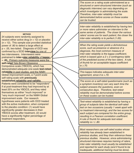
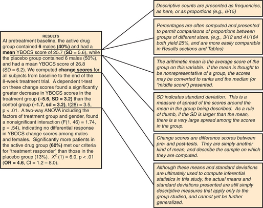
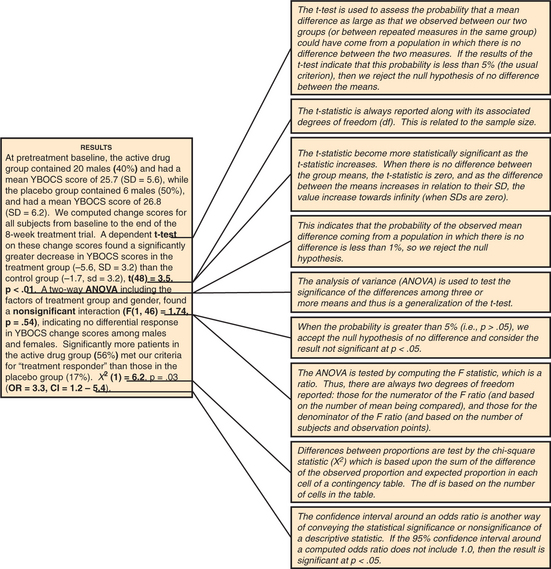
Figures 62-1 through 62-3 contain the annotated Method and Results sections for this fictional study, showing how the various psychometric statistics are presented in the Method section, while descriptive statistics are presented in the Method and Results sections, and inferential statistics are presented in the Results section (for definitions of terms used in these figures, refer to the section on statistical terms and their definitions).
Experiment-wise Error Rate
Researchers should test only a few carefully selected hypotheses (specified before collecting their data!) if their obtained p-values are to have any meaning. The more statistical tests you perform, the greater the chance of finding at least one significant by chance alone. Table 62-2 illustrates this phenomenon.
Table 62-2 Experiment-wise Error: Did the Researcher Find a Single Result Significant Solely by Chance?
| Number of Statistical Tests Performed at p < .05 | Probability of at Least One False-Positive Finding* |
|---|---|
| 1 | .05 |
| 2 | .09 |
| 3 | .14 |
| 4 | .18 |
| 5 | .22 |
| 6 | .26 |
| 7 | .30 |
| 8 | .33 |
| 9 | .36 |
| 10 | .41 |
| 15 | .53 |
| 20 | .64 |
| 30 | .78 |
| 40 | .87 |
| 50 | .92 |
One should not be impressed by a researcher who conducts eight t-tests, finds one significant at p < .05, and proceeds to interpret the findings as confirming his theory. Table 62-2 shows us that with eight statistical tests at p < .05, the researcher had a 33% chance of finding at least one result significant by chance alone.
Selecting an Appropriate Statistical Method
The two key determinants in choosing a statistical method are (1) your research goal, and (2) the level of measurement of your outcome (or dependent) variable(s). Table 62-3 illustrates the key characteristics of the various levels of measurement and provides examples of each.
| Level of Measurement | Description of Level | Examples |
|---|---|---|
| Continuous (also known as interval or ratio) | A scale on which there are approximately equal intervals between scores |
Once the level of measurement of your outcome variable has been determined, you will decide whether your research question will require you to compare two or more different groups of subjects, or to compare variables within a single group of subjects. Tables 62-4 and 62-5 will help you choose the appropriate statistical method once you have made these decisions. (Note that these tables consider only univariate statistical tests; multivariate tests are beyond the scope of this chapter.)
Table 62-4 Choosing an Appropriate Statistical Test to Compare Two or More Groups, Based on Your Research Goal, and the Level of Measurement of Your Outcome Measure
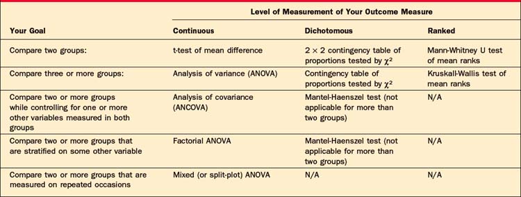
Table 62-5 Choosing an Appropriate Statistical Test for a Single Group of Subjects, Based on Your Research Goal, and the Level of Measurement of Your Outcome Measure
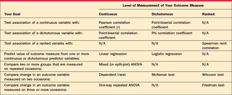
For example, if you want to conduct a study comparing a new drug to two control conditions, and your outcome measure is a continuous rating scale, Table 62-4 indicates that you would typically use the analysis of variance (ANOVA) to analyze your data. If you wanted to assess the associa-tion of two continuous measures of dissociation and anxiety in a single depressed sample, Table 62-5 indicates that you would usually select the Pearson correlation coefficient. (Note that the procedures listed for Ranked outcome measures are those typically referred to as “nonparametric tests.”)
The Importance of Assessing Statistical Power
A nonsignificant p-value is meaningless if the researcher studied too few subjects, resulting in low statistical power. Tables 62-6 through 62-8 will help you estimate the number of subjects required to have a reasonable chance (usually set at 80%, or power = .80) of detecting a true effect.
Table 62-6 Statistical Power: Did the Study Have Enough Subjects to Detect a True Significant Mean Difference between Two Groups?
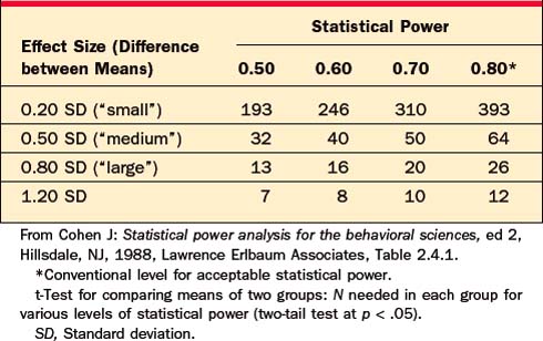
Table 62-7 Statistical Power: Did the Study Have Enough Subjects to Find a True Significant Difference in Proportions between Two Groups?
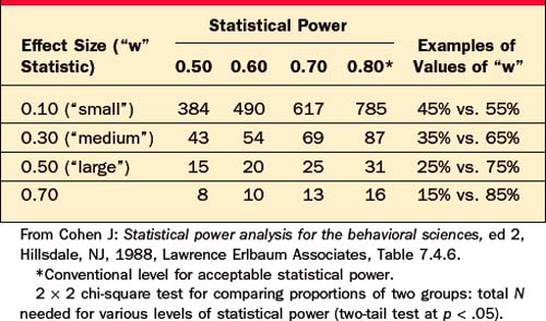
Table 62-8 Statistical Power: Did the Study Have Enough Subjects to Find a True Significant Correlation within a Group?
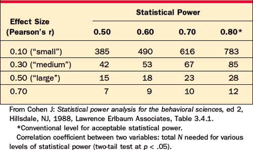
For example, a researcher reports that she has compared two groups of 12 depressed patients, and found that a new drug was not significantly better than placebo at p < .05, by t-test. However, this negative result is not informative, because Table 62-6 indicates that with only 12 subjects per group, this researcher had statistical power of less than .80 to detect even a “large” effect; that is, even if the drug were truly effective, this study had less than a 50/50 chance of finding a significant difference.
STATISTICAL TERMS AND THEIR DEFINITIONS
Correlation Matrix
This is a “Table” or “Matrix” of correlation coefficients for all variables of interest.
Effect Size
This is a measure of the practice significance of a treatment effect, as opposed to the statistical significance. For comparisons of two treatments, the most common effect size measure used is Cohen’s “d” (the mean difference between the groups in standard deviation units), with values of .20, .50, and .80 defined by Cohen as small, medium, and large effects in the behavioral sciences. Effect sizes are essential to computing statistical power (see Tables 62-6 to 62-8) and also form the basis of meta-analytic research.
Experiment-wise Error Rate
As more statistical tests are performed, you are more likely to find at least one of these tests significant by chance alone. Although you may perform each test at p < .05, your chance of finding one of many tests significant by chance alone is much higher than this nominal 5% level (see Table 62-2).
p-Value
Most journals require p < 0.05 for significance. If many statistical tests are performed in a study, a more conservative p-value can be used to minimize experiment-wise error (see Table 62-2). Caveat: Do not be overly impressed by very low p-values. Remember that all this tells you is the chance that the difference is probably not zero. Also, remember that, given enough subjects, this is easy to prove. Thus, a very low p-value does not necessarily indicate a large clinical effect, but instead represents that it is a very reliable effect. Check the effect size (the correlation coefficient squared, or the size of the t-statistic) to get an idea of the magnitude of the difference or relation.
Power
This reflects the probability of finding a true difference or relation between two or more measures with a given sample size. It is analogous to the sensitivity of a medical test. An analogy: The power of a telescope (i.e., the magnification) is analogous to the power of a study; both indicate the ability to detect even tiny objects or changes. If a study had little chance of finding a true difference between two drugs (say, with only two subjects per group), the power of the study would be nearly zero. If the study had almost no chance of missing a true difference (say, comparing the mean height of 10,000 2-year-olds with 10,000 18-year-olds), the power of the study would be nearly 1.00. Power of 0.80 is usually the minimum required by statisticians when designing a study. Caveat: Just as any tiny difference can be found to be significant just by having enough subjects, it is possible to find all but huge differences to be nonsignificant, simply by having few enough subjects! Be especially wary of false negatives in studies with few subjects (e.g., < 25 per group). Several literature reviews have found that the average behavioral science study has a power of only about 40% to detect a medium-sized effect! Consult Tables 62-6 to 62-8 to estimate the statistical power of a study.
Reliability
For scales or measures administered by a rater, the major question is, “Would this patient get the same score on this depression scale if Doctor A rated him, as if Doctor B rated him?” If the agreement was perfect for all patients, the reliability coefficient would be 1.00. If, on the other hand, there were a random relationship between the scores of the two raters, the interrater reliability would be 0.00. Reliability is necessary but not sufficient for a useful scale. Thus, a scale can be perfectly reliable, but have no validity for a particular purpose. For example, every time you ask me my phone number I will give you the same answer (perfect reliability); however, if you attempt to use my phone number to predict my anxiety level you will find a zero correlation (no validity). If a measure has no reliability (i.e., it is not reproducible), it has zero reliability. If it has perfect reliability, or repeatability, it has a reliability of 1.00.
CURRENT CONTROVERSIES AND FUTURE DIRECTIONS
Cohen J. Statistical power analysis for the behavioral sciences, ed 2. Hillsdale, NJ: Lawrence Erlbaum Associates, 1988.
Cohen J, Cohen P, West SG, Aiken LS. Applied multiple regression/correlation analysis for the behavioral sciences, ed 2. Mahwah, NJ: Lawrence Erlbaum Associates, 1983.
Gonick L, Smith W. The cartoon guide to statistics. New York: HarperCollins, 1993.
Gorsuch R. Factor analysis. Hillsdale, NJ: Lawrence Erlbaum Associates, 1983.
Green SB, Salkind NJ. Using SPSS for Windows and Macintosh: analyzing and understanding data, ed 4. Upper Saddle River, NJ: Pearson Prentice Hall, 2004.
Huff D, Geis I. How to lie with statistics. New York: WW Norton, 1954.
Keith TZ. Multiple regression and beyond. Boston: Pearson Educational, 2006.
Rosenthal R, Rosnow RL. Essentials of behavioral research: methods and data analysis, ed 2. New York: McGraw-Hill, 1991.
Tabachnick BG, Fidell LS. Using multivariate statistics, ed 4. Boston: Allyn & Bacon, 2001.