[level-membership-for-psychiatry-category]
CHAPTER 61 Psychiatric Epidemiology
OVERVIEW
Epidemiology is based on two fundamental assumptions: first, that human disease does not occur at random, and second, that human disease has causal and preventive factors that can be identified through systematic investigation of different populations in different places or at different times. By measuring disease frequency, and by examining who gets a disease within a population, as well as where and when the disease occurs, it is possible to formulate hypotheses concerning possible causal and preventive factors.1
CRITERIA FOR ASSESSMENT INSTRUMENTS
Reliability is the degree to which an assessment instrument produces consistent or reproducible results when used by different examiners at different times. Lack of reliability may be the result of divergence between observers, imprecision in the measurement tool, or instability in the attribute being measured. Interrater reliability (Table 61-1) is the extent to which different examiners obtain equivalent results in the same subject when using the same instrument; test-retest reliability is the extent to which the same instrument obtains equivalent results in the same subject on different occasions.
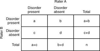 |

where Po is the observed agreement and Pc is an agreement due to chance. Po = (a + d)/n and Pc = [(a + c)(a + b) + (b + d)(c + d)]/n2. Calculation of the ICC is more involved and is beyond the scope of this text.
Assessment of New Instruments
If we assume that a reliable criterion instrument that pro-vides valid results exists, the assessment of a new measurement instrument would involve comparing the results of the new instrument to those of the criterion instrument. The criterion instrument’s results are considered “true,” and a judgment of the validity of the new instrument’s results are based on how well they match the criterion instrument’s (Table 61-2).
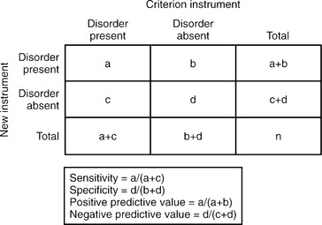 |
For any given instrument, there are tradeoffs between sensitivity and specificity, depending on where the threshold limits are set to distinguish “case” from “non-case.” For example, in the Hamilton-Depression Scale (HAM-D) instrument, the cutoff value for the diagnosis of MDD (often set at 15) would determine whether an individual would be identified as “case” or “non-case.” If the value were instead set at 5, which most clinicians would consider “normal” or not depressed, the HAM-D would be an unusually sensitive instrument (e.g., using a structured clinical interview as the criterion instrument) since most anyone evaluated with even a modicum of depressive thinking would be considered a “case” as would anybody typically considered to have major depression. However, the test would not be especially specific, since it would be poor at identifying those without depression. Conversely, if the cutoff value were set at 25, sensitivity would be low but the specificity high.
Study Designs
Descriptive Studies
The weakest of all study designs, these studies simply describe the health status of a population or of a number of subjects. Case series are an example of descriptive studies, and are simply descriptions of cases, without a comparison group. They can be useful for monitoring unusual patients, and in generating hypotheses for future study. One example is Teicher and colleagues’ 1990 case series of six patients who developed suicidal ideation on fluoxetine, which informed future studies that ultimately led to black box warnings for all antidepressants.2 Case series can also be misleading, though, as in the early 1980s when physicians began describing male homosexuals with depressed immune systems. The use of amyl nitrate–based sexual stimulants was a suspected cause, and studies on the effects of amyl nitrates on the immune system were under way when HIV was discovered.
Case-Control Studies
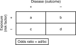
In case-control studies, subjects are selected based on whether they have the outcome (case) or not (control), and their exposures are then determined by looking backward in time. For this reason, they are also called retrospective studies, since they rely on historical records or recall. This type of study design is appropriate for rare diseases or for those with long latencies, and they can also be used to study possible risk factors. Problems with case-control studies include recall bias (which occurs if cases and controls recall past exposures differently) and difficulty in selecting controls. Ideally, one wants controls who are exactly matched to the cases in all other exposures except for the risk factor in question (Table 61-3). Thus, controls should be matched for a variety of factors, for example, gender, socioeconomic status (SES), smoking status (unless that is what is being studied), and alcohol use. For case-control studies, an odds ratio is used to determine whether the outcome is more likely in those with the exposure, or in those without one, and it is an approximation of their relative incidence rates.
Table 61-3 Association Between Risk Factors and Outcome in Case-Control and Cohort Studies
 |
Cohort Studies
Examples of cohort studies include the Framingham Heart Study (which has followed generations of residents from Framingham, Massachusetts) and the Nurses Health Study (which has followed a national sample of nurses with annual questionnaires). One classic study in Britain followed 35,445 British physicians and found that among smokers, the incidence of lung cancer was 1.30 per 1,000, but only 0.07 for nonsmokers.3 The relative risk was therefore 1.30/0.07 = 18.6, indicating that smokers had more than 18 times the risk of developing lung cancer than nonsmokers.
DEVELOPMENT OF ASSESSMENT TOOLS
Case Definition
In 1972, Cooper and colleagues4 published a United States/United Kingdom study that showed high variability in the diagnosis of psychotic disorders. It highlighted the need for having explicit operational criteria for case identification. The development of such diagnostic criteria with the publishing of the Diagnostic and Statistical Manual of Mental Disorders, Third Edition (DSM-III) in 1980 represented a notable step toward increasing the reliability and validity of psychiatric diagnoses.
CONTEMPORARY STUDIES IN PSYCHIATRIC EPIDEMIOLOGY
The Baseline National Comorbidity Survey (NCS)
The NCS General Findings
DSM-III-R disorders were more prevalent than had been expected. About 48% of the sample reported at least one lifetime disorder, and 30% of respondents reported at least one disorder in the 12 months preceding the interview. The most common disorders were major depression and alcohol dependence, followed by social and simple phobias. As a group, substance use and anxiety disorders were more prevalent than affective disorders, with approximately one in four respondents meeting criteria for a substance use disorder in their lifetime, one in four for an anxiety disorder, and one in five respondents for an affective disorder (Table 61-4).
Table 61-4 Lifetime and 12-Month Prevalence Estimates for Psychiatric Disorders, NCS Results
| Lifetime Prevalence Estimate (%) | 12-Month Prevalence Estimate (%) | |
|---|---|---|
| Major depression | 17.1 | 10.3 |
| Mania | 1.6 | 1.3 |
| Dysthymia | 6.4 | 2.5 |
| Generalized anxiety disorder | 5.1 | 3.1 |
| Panic disorder | 3.5 | 2.3 |
| Social phobia | 13.3 | 7.9 |
| Simple phobia | 11.3 | 8.8 |
| Agoraphobia without panic | 5.3 | 2.8 |
| Alcohol abuse | 9.4 | 2.5 |
| Alcohol dependence | 14.1 | 7.2 |
| Drug abuse | 4.4 | 0.8 |
| Drug dependence | 7.5 | 2.8 |
| Antisocial personality disorder | 2.8 | — |
| Nonaffective psychosis* | 0.5 | 0.3 |
* Nonaffective psychosis: schizophrenia, schizophreniform disorder, schizoaffective disorder, delusional disorder, and atypical psychosis.
Source: Adapted from Tsuang and Tohen (2002).5
NCS-Replication Survey (NCS-R)
Mental Health Services Utilization
From the NCS to the NCS-R, there was no change in the overall prevalence of mental disorders, but the rate of treatment increased in the past decade. Among patients with a psychiatric disorder, 20.3% received treatment between 1990 and 1992 compared to 32.9% between 2001 and 2003 (p < 0.001). Nevertheless, most patients with mental disorders in the NCS-R study still did not receive treatment. For those who did, there was significant delay, ranging from 6 to 8 years for mood disorders and 9 to 23 years for anxiety disorders. The unmet need of mental health services has been greatest in traditionally underserved groups (including elderly persons, racial-ethnic minorities, residents of rural areas, and those with low incomes or without insurance).
The European Study of the Epidemiology of Mental Disorders (ESEMeD) Project
The ESEMeD is a cross-sectional epidemiological study, conducted between January 2001 and August 2003, that assessed the psychiatric epidemiology of 212 million noninstitutionalized adults from Belgium, France, Germany, Italy, the Netherlands, and Spain.6 Individuals were assessed in-person at their homes using computer-assisted psychiatric interview (CAPI) instruments, and data from 21,425 respondents were collected. A stratified, multistage, clustered area, probability sample design was used to analyze the data.
EPIDEMIOLOGY OF MAJOR PSYCHIATRIC DISORDERS
Schizophrenia
Risk Factors
Genetic loading is a robust risk factor for schizophrenia (Table 61-5). The prevalence of schizophrenia in a monozygotic twin of a schizophrenia patient is 50%, and 15% in a dizygotic twin. The prevalence for a child with two schizophrenic parents is 46.3%, and 12.8% for a child with one schizophrenic parent.
Table 61-5 Prevalence of Schizophrenia in Specific Populations
| Population | Prevalence (%) |
|---|---|
| General population | 0.3 |
| First-degree relatives of parents of schizophrenic patients | 5.6 |
| Children with one schizophrenic parent | 12.8 |
| Dizygotic twins of a schizophrenic patient | 15.0 |
| Children of two schizophrenic parents | 46.3 |
| Monozygotic twins of a schizophrenic patient | 50.0 |
Bipolar I Disorder
Risk Factors
Both Epidemiology Catchment Area (ECA) and NCS studies showed that there is no gender difference in the prevalence of bipolar disorder. Some studies conducted before 1980 showed a higher prevalence of bipolar disorder in the upper socioeconomic classes, but there has been no evidence for that in recent studies. Bipolar I disorder occurs at much higher rates in first-degree biological relatives of persons with bipolar I disorder than it does in the general population. Family, adoption, and twin studies clearly support the evidence that bipolar disorder is genetically transmitted. The lifetime risks of suffering from bipolar disorder in relatives of bipolar probands are 40% to 70% in monozygotic co-twins, 5% to 10% in first-degree relatives, and 0.5% to 1.5% in non–blood-related individuals. Individuals who are cohabitating, divorced, or never married are more likely to suffer from bipolar disorder compared to those who are married. Both the ECA and the NCS studies found that there were no race differences in the prevalence of bipolar disorder.
1 Hennekens CH, Buring JE;1987, Little, Brown Boston 73-100
2 Teicher MH, Glod C, Cole JO. Emergence of intense suicidal preoccupation during fluoxetine treatment. Am J Psychiatry. 1990;147:207-210.
3 Doll R, Hill AB. Mortality in relation to smoking: ten years’ observations of British doctors. Br Med J. 1964;1(5395):1399-1410. 1(5396):1460-1467
4 Cooper JE, Kendell RE, Gurland BJ, et al. Psychiatric diagnosis in New York and London. London: Oxford University Press, 1972.
5 Tsuang MT, Tohen M. Textbook in psychiatric epidemiology, ed 2, New York: Wiley; 2002:343-479.
6 ESEMeE/MHEDEA 2000 Investigators. Prevalence of mental disorders in Europe: results from the European Study of the Epidemiology of Mental Disorders (ESEMeD) project. Acta Psychiatr Scand. 2004;109(suppl 420):21-27.
[/level-membership-for-psychiatry-category][not-level-membership-for-psychiatry-category]
CHAPTER 61 Psychiatric Epidemiology
OVERVIEW
Epidemiology is based on two fundamental assumptions: first, that human disease does not occur at random, and second, that human disease has causal and preventive factors that can be identified through systematic investigation of different populations in different places or at different times. By measuring disease frequency, and by examining who gets a disease within a population, as well as where and when the disease occurs, it is possible to formulate hypotheses concerning possible causal and preventive factors.1
CRITERIA FOR ASSESSMENT INSTRUMENTS
Reliability is the degree to which an assessment instrument produces consistent or reproducible results when used by different examiners at different times. Lack of reliability may be the result of divergence between observers, imprecision in the measurement tool, or instability in the attribute being measured. Interrater reliability (Table 61-1) is the extent to which different examiners obtain equivalent results in the same subject when using the same instrument; test-retest reliability is the extent to which the same instrument obtains equivalent results in the same subject on different occasions.
|
where Po is the observed agreement and Pc is an agreement due to chance. Po = (a + d)/n and Pc = [(a + c)(a + b) + (b + d)(c + d)]/n2. Calculation of the ICC is more involved and is beyond the scope of this text.
Assessment of New Instruments
If we assume that a reliable criterion instrument that pro-vides valid results exists, the assessment of a new measurement instrument would involve comparing the results of the new instrument to those of the criterion instrument. The criterion instrument’s results are considered “true,” and a judgment of the validity of the new instrument’s results are based on how well they match the criterion instrument’s (Table 61-2).
|
[/not-level-membership-for-psychiatry-category]
