CHAPTER 2
Acquisition and interpretation of biochemical data
CHAPTER OUTLINE
FACTORS AFFECTING TEST RESULTS
Comparison of observed results with reference limits
Comparison of results with previous values
Prevalence and predictive value
Practical applications of the predictive value model
INTRODUCTION
It was emphasized in Chapter 1 that all investigations in medicine should be performed to answer specific questions. Biochemical data obtained must be considered in relation to the reason for the request, and against the background of an understanding of the relevant normal physiological and biochemical mechanisms and the way in which these respond to disease. One of the objectives of any laboratory is to ensure these data are available in a timely manner, and generated efficiently. The achievement of this goal requires careful attention to every step in the process, from the ordering of the investigation, the collection of the specimen(s) required, their transport to the laboratory and analysis, to the delivery of a report to the clinician, appropriate action being taken and the effects of this action being assessed. Amongst these many steps, the interpretation of data by clinical biochemists adds considerably to the value of the data. The workload of most laboratories is so great that it would be impossible (as well as being unnecessary) to add such comments to all reports (e.g. where the results are clearly normal). Interpretative comments (which may be individual or rule-based) are more likely to be required for more unusual tests, and for requestors who have only limited experience of the investigation in question. Typical reports requiring more detailed interpretation include those with borderline data, results that are not consistent with the clinical findings, apparently contradictory data and changes in biochemical variables during dynamic function tests.
THE TEST REQUEST
The first step in performing a biochemical investigation is for a request form to be completed, often electronically, which prompts the collection of the appropriate specimen(s) and instructs the laboratory on the investigations(s) to be performed. Depending upon the reason for the request, the expertise of the clinician and the practice of the laboratory, the request may simply be for one or more specified analyses on a body fluid; for a set (often referred to as a ‘profile’) of standard investigations (e.g. ‘thyroid function tests’); for a more involved procedure such as a dynamic function test involving the collection of serial samples following a specific stimulus, or an open request to perform whatever assays are deemed appropriate by the laboratory staff to answer the question posed in the request. The majority of biochemical test requests fall into the first two categories.
The information that is required when a test is requested is summarized in Table 2.1.
TABLE 2.1
Information required when requesting a biochemical investigation
| Information | Reason |
| Patient’s name, identifying (e.g. hospital) numbera, date of birth and sex | Identification and (age, sex) interpretation of results |
| Home address for primary care patients | Address may be useful if grossly abnormal results are found |
| Return address (e.g. ward, clinic, surgery; telephone/pager number if urgent) | Delivery of report |
| Name of clinician (and telephone/pager number) | Liaison Audit Billing |
| Clinical details (including drug treatment) | Justification of request Audit Interpretation Selection of appropriate assays Choice of analytical method (to avoid drug interference) |
| Test(s) requested | Instruction to analyst |
| Sample(s) required | Instruction to phlebotomist |
| Date (and timeb if appropriate) | Identification Interpretation (with timed/sequential requests) |
a In the UK, it is mandatory to supply the National Health Service Number.
b It is good practice also to record the time at which the specimen and request is received in the laboratory.
FACTORS AFFECTING TEST RESULTS
The generation of biochemical data is potentially subject to error at every stage in the process. It is essential that the sources of error are identified and understood, so that their effects can be minimized.
The sources of errors in biochemical tests are conventionally described in three categories:
• analytical: these may be random (e.g. due to the presence of an interfering substance in the specimen) or systematic (e.g. because of a bias in the method)
• postanalytical: that is, occurring during data processing or transmission, or in relation to the interpretation of the data.
Preanalytical factors
Preanalytical factors may appear to be beyond the remit of clinical biochemists, but accreditation bodies are increasingly expecting laboratories to take responsibility for all aspects of testing. Laboratories should ensure that clinicians requesting investigations and the staff responsible for collecting the specimens understand the problems that can arise, so that specimens are collected and transported appropriately.
Preanalytical factors fall into two categories: those that relate to the specimen obtained for analysis (technical factors) and those that relate directly to the patient (biological factors).
Technical factors
These include:
• correct identification of the patient
• appropriate preparation of the patient where necessary
• collection of the specimen into an appropriate container with the correct anticoagulant or preservative
• accurate labelling of the specimen container after the sample has been collected (not before, as this carries a higher risk of a specimen being put into a container bearing another patient’s name). Primary labelling of the sample with a barcode at source reduces the risk of mislabelling in the laboratory
• rapid and secure transport to the laboratory. Some specimens need to be transported under special conditions, for example arterial blood for ‘blood gases’ in a sealed syringe in an ice-water mixture; requests for blood, urine or faecal porphyrins must be protected from light.
Care must be taken during specimen collection to avoid contamination (e.g. with fluid from a drip), haemolysis of blood or haemoconcentration (due to prolonged application of a tourniquet). Appropriate precautions are also required during the collection and transport of urine, faeces, spinal fluid or tissue. Specimens known to be infective (e.g. from patients carrying the hepatitis B or HIV viruses) are occasionally handled specially, but it is good practice to handle all specimens as if they were potentially hazardous.
On receipt in the laboratory, the patient’s name and other identifiers on the specimen must be checked against these details on the request form, whether paper or electronic. The specimen and form should then be labelled with the same unique number. As electronic requesting becomes more common, the majority of specimens are now being labelled with a unique barcode at source. Secondary containers (e.g. aliquots from the primary tube) should also be identified with patient details and the same unique number as the primary container. Automated preanalytical robotics and track systems can minimize the number of manual interventions required during sample handling, thereby minimizing risk of errors. All these processes are facilitated if computer systems in hospitals or surgeries have electronic links to the laboratory information system.
Laboratories should have written protocols (standard operating procedures) for the receipt and handling of all specimens to ensure the positive identification of specimens throughout the analytical process.
Biological factors
Numerous factors directly related to the patient can influence biochemical variables, in addition to pathological processes. They can conveniently be divided into endogenous factors, intrinsic to the patient, and exogenous factors, which are imposed by the patient’s circumstances. They are summarized in Table 2.2.
TABLE 2.2
Some biological factors affecting biochemical variables
| Factor | Example |
| Endogenous | |
| Age | Cholesterol Alkaline phosphatase Urate |
| Sex | Gonadotrophins Gonadal steroids |
| Body mass | Triglycerides |
| Exogenous | |
| Time | Cortisol (daily) Gonadotrophins (in women, catamenial) 25-Hydroxyvitamin D (seasonal) |
| Stress | Cortisol Prolactin Catecholamines |
| Posture | Renin Aldosterone Proteins |
| Food intake | Glucose Triglycerides |
| Drugs | see Table 2.3 and text |
In addition, all biochemical variables show some intrinsic variation, tending to vary randomly around the typical value for the individual.
Endogenous factors
Age
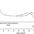
The reference values (mentioned in more detail later in the chapter) for many biochemical variables do not vary significantly with age during adult life. Some, however, are different during childhood, particularly in the neonatal period. A well-known example is plasma alkaline phosphatase activity, which is higher in children, particularly during the pubertal growth spurt, than in adults. Plasma cholesterol concentrations tend to increase with age, but may fall slightly over the age of 70; plasma urate concentrations tend to rise with age. Given that renal function tends to decline with age, it might be anticipated that mean plasma creatinine concentrations would rise with age, but the tendency for loss of muscle bulk in the elderly has a balancing effect. Other age-related changes are discussed elsewhere in this book.
Sex
Apart from the obvious differences in plasma gonadal hormone concentrations between adult men and women, other analytes demonstrate sex-related differences in concentration, often because their metabolism is influenced by gonadal hormones. Thus, total cholesterol concentrations tend to be higher in healthy men than in women until the menopause, after which concentrations in women tend to rise. In general, sex-related differences in biochemical variables are less between boys and girls prepubertally, while the differences between adult males and females decrease after the menopause.
When age and sex are important determinants of the level of a biochemical variable, measurements in patients should be considered in relation to age- and sex-related reference values, if valid conclusions are to be drawn.
Changes in many biochemical variables occur during pregnancy and, where necessary, measurements must be compared with reference values appropriate to the stage of gestation. The clinical biochemistry of pregnancy is considered in detail in Chapter 22.
Ethnic origin
Plasma creatine kinase activity tends to be higher in people of sub-Saharan African descent than Caucasians (typically up to three times the upper reference limit; people of southern Asian origin may have intermediate values), but otherwise, there are no significant differences in the typical values for most biochemical variables between individuals of different ethnic origin living in the same region.
Body mass
Obese individuals tend to have higher plasma insulin and triglyceride concentrations than lean individuals, with an increased risk of developing type 2 diabetes and cardiovascular disease. Creatinine production is related to muscle bulk and plasma concentration may be above the usual reference range in a muscular individual, despite having a normal glomerular filtration rate. Twenty-four hour urinary excretion of many substances is greater in people of higher body mass. On the whole, however, body mass has little effect on the concentrations of substances in body fluids, although, of course, it is an important determinant of the total quantities of many substances in the body.
Exogenous factors
Many exogenous factors can have profound influences on the concentrations of biochemical variables even in healthy individuals. They include the time of day, stress, posture, fasting status, drugs, exercise and concurrent illness (see Tables 2.2 and 2.3).
TABLE 2.3
Some examples of in vivo effects of drugs on biochemical variables
| Drugs | Effect | Mechanism |
| Glucocorticoids | Decreased plasma cortisol | Suppression of ACTH secretion |
| Thiazide diuretics | Decreased plasma potassium | Increased renal potassium excretion |
| Oestrogens | Increased plasma total thyroxine | Increased synthesis of binding proteins |
| Phenytoin, phenobarbitone, alcohol | Increased plasma γ-glutamyltransferase | Increased enzyme synthesis (enzyme induction) |
Time-dependent changes
Rhythmic changes occur in many physiological functions and are reflected in changes in the levels of biochemical variables with time. The time base may be diurnal (related to the time of day, but usually nycthemeral, i.e. related to the sleep–wake cycle), catamenial (relating to the menstrual cycle) or seasonal. In addition, some hormones are secreted in sporadic bursts (e.g. growth hormone); when this occurs, it may be helpful to collect several blood samples over a short period of time and to base clinical decisions on the mean value.
The best known analyte having a diurnal variation in concentration is cortisol. Its concentration is at a nadir at about midnight, rises rapidly to reach a peak at 08.00–09.00 h and then declines throughout the day. Observed values must be compared with reference values for specific times, with sampling at expected peak or trough times being the most informative. Other analytes showing a diurnal rhythm (but to lesser extents) include thyroid stimulating hormone, testosterone and prolactin.
Some analytes show regular variations with a different time base. In women, during the reproductive years, the menstrual cycle is associated with regular changes in the concentrations of gonadotrophins, oestrogens and progesterone. Measurements made for diagnostic purposes must be made at the appropriate time in the cycle: for example, an increase in plasma progesterone concentration seven days before the onset of the next menstrual period is due is taken as an indication that ovulation has occurred.
Plasma 25-Hydroxycholecalciferol concentration varies with the season, being higher in summer than in winter.
Stress
Concern for the patient dictates that stress should be minimized at all times, but this is particularly important in relation to blood sampling for those analytes with concentrations that are responsive to (usually by increasing) stress. Pituitary and adrenal hormones are particularly affected. Thus plasma adrenocorticotropic hormone (ACTH), cortisol, prolactin, growth hormone and catecholamine concentrations all rise in response to stress. Indeed, this effect is utilized in investigations of pituitary function. However, avoidance of stress is vital when collecting specimens for the measurement of these hormones under other circumstances.
Posture
Posture has a significant effect on a wide range of analytes. The best known of these are plasma renin activity and aldosterone concentration. Both are higher in the standing than the recumbent (or even sitting) position, particularly shortly after the change in posture, as a result of a decrease in renal blood flow.
The effect of posture on certain other analytes is less well appreciated. When people are upright, there is a greater tendency for fluid to move from the vascular to the interstitial compartment than when they are recumbent. Small molecules and ions in solution move with water, but macromolecules and smaller moieties bound to them do not. As a result, the concentrations of proteins, including lipoproteins, and of protein-bound substances, for example thyroid and other hormones, calcium and iron, tend to be approximately 10% higher when an individual is in the upright position than when recumbent. Intermediate values occur when sitting. This effect may be relevant when values obtained from individuals when they are outpatients are compared with values obtained when they are inpatients.
Food intake
The concentrations of many analytes vary in relation to food intake. Frequently encountered examples include glucose, triglycerides and insulin, the plasma concentrations of which all increase following a meal, so that they should usually be measured in the fasting state, unless the effect of recent intake (as in the glucose tolerance test) is being examined. Some specific dietary constituents can affect biochemical variables; consumption of red meat in the hours before venepuncture may increase plasma creatinine concentrations by as much as 30% from fasting values. A protein-rich meal results in increased urea synthesis and increases plasma urea concentration. Long-term dietary habits can also significantly affect biochemical variables (e.g. cholesterol).
The urinary excretion of many substances is highly dependent on their intake and, although some laboratories publish reference ranges for them, they are very wide. In assessing the significance of the excretion of substances in the urine, it is important to consider their intake and thus their expected excretion if renal function is normal. Thus, for example, a low urinary sodium excretion is a normal response to sodium depletion.
Drugs
Drugs, whether taken for therapeutic, social or other purposes, can have profound effects on the results of biochemical tests. These can be due to interactions occurring both in vivo and in vitro.
In vivo interactions occur more frequently. They can be due to direct or indirect actions on physiological processes or to pathological actions. There are numerous examples in each category. Some of the better known physiological interactions are indicated in Table 2.3. Others are discussed elsewhere in this book.
Pathological consequences of drug action in vivo can be idiosyncratic (unpredictable) or dose related. A measurable biochemical change may be the first indication of a harmful effect of a drug, and biochemical tests are widely used to provide an early indication of possible harmful effects of drugs, both for those in established use (e.g. measurement of serum creatine kinase activity in patients being treated with statins) and in drug trials.
Drugs can also interfere with analyses in vitro (this is strictly an analytical factor, but is mentioned here for completeness), for example by inhibiting the generation of a signal or by cross-reacting with the analyte in question and giving a spuriously high signal. This field is well documented, but the introduction of new drugs means that new examples of this source of error are continually being described.
Other factors
Exercise can cause a transient increase in plasma potassium concentration and creatine kinase activity; the latter used to be a potential confounding factor in the diagnosis of myocardial infarction in a patient who had developed chest pain during exercise before cardiac-specific troponin measurement was introduced. Even uncomplicated surgery may cause an increase in creatine kinase as a result of muscle damage, and tissue damage during surgery can also cause transient hyperkalaemia. Major surgery and severe illness can elicit the ‘metabolic response to trauma’ (see Chapter 20), which can lead to changes in many biochemical variables.
Intrinsic biological variation
The contributions to biological variation discussed thus far are predictable, and either preventable or can be allowed for in interpreting test results. However, levels of analytes also show random variation around their homoeostatic set points. This variation contributes to the overall imprecision of measurements and must also be taken into account in the interpretation of test results. It is also relevant to the setting of goals for analytical precision (see below).
Intrinsic biological variation can be measured by collecting a series of specimens from a small group of comparable individuals over a period of time (typically several weeks) under conditions such that analytical imprecision is minimized. The specimens should be handled identically and analysed in duplicate, using an identical technique (e.g. the same instrument, operator, calibrators and reagents). This may either be done at the time the specimens are collected or in a single batch. If the latter approach is adopted, the specimens must be stored in such a way that degradation of the analyte is prevented (e.g. by freezing at a sufficiently low temperature). Using a single batch procedure is preferable as it eliminates between-run analytical variation.
If the specimens are analysed in a single batch, the analytical imprecision (see below) can be calculated from the differences in the duplicate analyses and is given by:
where SD is the standard deviation and n is the number of pairs of data. If, however, specimens are analysed at the time they are taken, the analytical imprecision must be calculated from replicate analyses of quality control samples.
The standard deviation of a single set of data from each individual is then calculated after excluding any outliers (‘fliers’) using an appropriate statistical test. This standard deviation will encompass both analytical variation and the intraindividual variation (SDI), such that:
Since SDA is known, the intraindividual variation can then be calculated. It is also possible to calculate the interindividual variation (SDG, due to the difference in the individual homoeostatic set points for the analyte between each member of the group) by calculating the SD for all single sets of data for all subjects in the group, since this SD is given by:

The calculations required can be performed using a nested analysis of variance technique as provided in many statistical software packages. An alternative approach is to calculate coefficients of variation (CV) (given by (SD × 100)/mean). Values for CV can be substituted for SD in these formulae because the means are similar.
Some typical values of biological variation for frequently measured analytes are given in Table 2.4. (A reference to a more extensive list is provided in the Further reading section at the end of the chapter.) It should be noted that, while in most instances the interindividual variation is greater than the intraindividual variation, this is not always the case. When it is not, it means that the extent of natural variation around individuals’ homoeostatic set points is more than the range of variation between these set points. The relative sizes of intra- and interindividual variation have important consequences for the interpretation of analytical data in relation to reference ranges, as will be discussed later in the chapter.
TABLE 2.4
Biological and analytical variation and consequent desirable analytical performance parameters for some frequently measured constituents of plasma expressed as coefficients of variation (CV = (SD × 100)/mean)
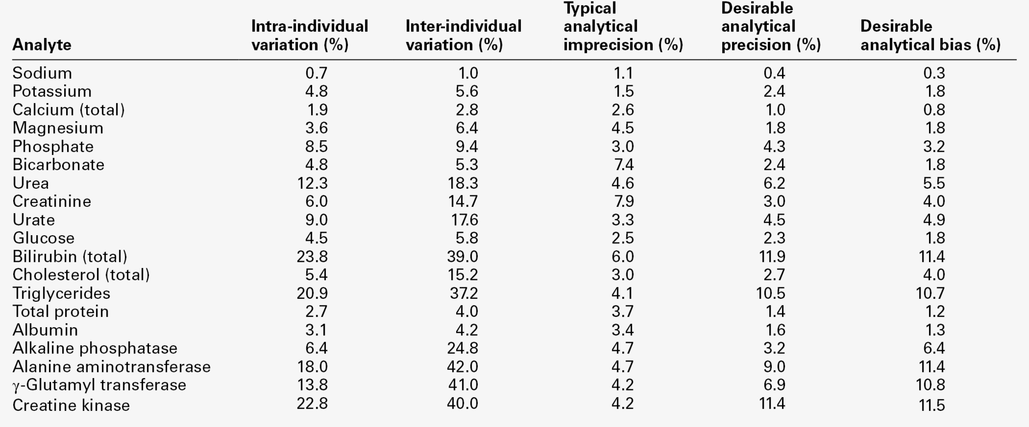
Data from various sources, including UKNEQAS (UK National External Quality Assurance Scheme) website and Ricos et al. on Westgard QC website (see Further reading).
Analytical factors
It is clearly essential that every effort is made to reduce the possibility of errors arising during analysis. A rigorous quality assurance programme (discussed in Chapter 3), is required to ensure the quality of results. The production of reports and their transmission to the requesting clinician are discussed below (see Postanalytical factors).
Test methods and procedures must be selected to allow adequate performance. Some of the important factors that impinge on performance will now be considered. The question of what is adequate performance will also be discussed. It should be appreciated that deciding on the standards for performance of individual assays requires an appreciation of all the factors involved: efforts to reduce specimen volume (an important consideration in paediatric, and particularly neonatal, practice) may affect accuracy and precision; these may also be influenced by a requirement to achieve a very rapid turnaround time. Cost, instrumentation and staff skill mix are other important factors.
Analytical range
The test selected must be capable of measuring the analyte in question over the whole range of concentrations that may be expected to occur. Measuring large quantities of an analyte is usually easier than measuring small quantities (though dilution of the sample may be necessary to bring the concentration within the range of acceptable performance, i.e. to avoid nonlinearity of signal to concentration). Note, however, that if dilutions are to be employed, their validity must be established by appropriate studies to demonstrate that dilution, per se, does not affect the relationship between analyte concentration and the signal generated. It is not always possible to design an assay that has a low enough detection limit (i.e. the lowest level of the analyte that can be reliably distinguished from zero, usually taken as the mean signal generated by zero standards plus two standard deviations); this has been a particular problem with the analysis of certain hormones, the plasma concentrations of which are in the nano- or even picomolar range, but is becoming less so with the introduction of more sensitive assay techniques.
For some analytes, the need to be able to measure concentrations over very wide ranges can pose technical problems, for example the ‘high dose hook effect’ with immunoassays for prolactin and human chorionic gonadotrophin. This term refers to the decrease in signal that occurs at high concentrations as a result of binding sites on the capture and labelled antibodies being occupied by separate molecules of the analyte rather than these causing crosslinking between them (the usual situation when the antibodies are in excess). For C-reactive protein (CRP) in serum, the requirement to be able to measure concentrations accurately in two different ranges (‘high sensitivity’ CRP as a cardiovascular risk marker or marker of neonatal sepsis and CRP as an inflammatory marker) has led to the introduction of separate assays for each of the two ranges of concentration.
Accuracy and bias
Accuracy reflects the ability of an assay to produce a result that reflects the true value. Inaccuracy is the numerical difference between the mean of a set of replicate measurements and the true value. The term ‘bias’ is often preferred to ‘inaccuracy’ in laboratory medicine as it implies a persistent characteristic rather than an occasional effect. It is due to systematic error (cf. precision, below) and can be positive (the result is higher than the true result) or negative (lower than the true result), and constant (being the same absolute value throughout the analytical range) or proportional (having the same relative value to the true result).
Ideally, analyses should be without bias, but, provided that its extent and characteristics are known, the predictability of bias makes it less of a problem in the interpretation of laboratory data than imprecision.
Precision
Precision is a reflection of reproducibility. Imprecision is defined as the standard deviation for a series of replicate analyses (i.e. made on the same sample, by the same method, under identical conditions). For many analytes it is very low, giving coefficients of variation (CV, defined as (SD × 100)/mean value) of 1% or less. For others it is higher, giving CVs as high as 5%. The median imprecisions for some serum analytes, as achieved by a group of laboratories in the UK, are given in Table 2.4.
Imprecision in analysis can never be entirely eliminated. Such analytical variation is an important factor to be borne in mind when interpreting the results of laboratory tests, as discussed later.
Analytical variation or imprecision can be measured by performing repeated analyses on a single sample and calculating the standard deviation of the results, or by doing duplicate measurements on a series of samples as described in the section on biological variation, above. Imprecision tends to be highest when the signal generated by an assay (e.g. a colour change or electric potential) is low. To be of value in interpreting results, imprecision should be determined over a range of concentrations and particularly in the region of critical values (decision levels), where a small change in a result can lead to a significant change in management of the patient.
Specificity and interference
Specificity is the ability of an assay to measure only the analyte it purports to measure. Most assays are highly specific, but exceptions do occur, both owing to endogenous substances and to drugs that can give a signal in the assay and cause the concentration/activity to appear higher or lower than it is. A detailed discussion of this topic is beyond the scope of this chapter. Some important examples are mentioned elsewhere in this book and further information is available from the bibliography. Interference is a related, but separate problem, in that a substance alters the signal given by the analyte in question, but does not generate a signal itself.
Practicalities: what is desirable performance?
In their enthusiasm to perfect analytical methods, clinical biochemists must be careful not to lose sight of the application of their work. A result is of no value if its bias or imprecision render it dangerously unreliable; neither is it of value if the method is practically too complicated or too expensive to be useful, or if it takes so long to perform that the need for the result has passed by the time it becomes available.
What is required of a test is that it should be capable of providing a result that will answer the question that is posed. To give a simple example, if the requirement is to confirm that a patient with the typical clinical features of diabetic ketoacidosis does indeed have this condition, what is needed is a rapid test that will confirm the presence of hyperglycaemia. In this context, it is of little relevance whether the blood glucose concentration is 30 or 35 mmol/L. But if a glucose tolerance test is required to establish (or refute) a diagnosis of diabetes because the clinical features are equivocal, time is of little concern, but the precision and accuracy are of paramount importance. Imprecision or bias may lead to the diagnosis being missed or a patient being classified as having diabetes and managed as if he had the condition when he does not.
In practice, it is rarely necessary to sacrifice accuracy and precision for the sake of a result being available rapidly. Providing that they are used competently, and in accordance with standard operating procedures, many rapid methods, including point-of-care (near-patient) testing instruments, using ‘dry chemistry’ techniques, are intrinsically as reliable as traditional laboratory-based procedures. But, although clinical biochemists rightly strive to increase the accuracy and precision of assays, there must come a point where further efforts may not result in significant improvements in the reliability of data or their value when applied to patient care. The question: ‘What is desirable performance?’ needs examination in some detail.
Analytical goals
Numerous strategies have been applied to the setting of desirable standards for the performance characteristics of laboratory tests or ‘analytical goals’. These have been based, for example, on the opinions of clinical users, of laboratory-based experts, on imprecision data, on arbitrary fractions of the reference range etc. The most widely accepted strategy for defining analytical goals is based on data on analytical imprecision in the assay and biological variation for the analyte. The desirable goal is that analytical imprecision should be less than or equal to half the intraindividual biological variation.
Expressing imprecision as coefficients of variation (CV), the goal is thus: CVA ≤ 0.5 × CVI, where CVA is the CV for analytical imprecision and CVI is the CV for intraindividual variation. Since the overall imprecision is equal to the square root of the sum of the squares of individual imprecisions, i.e:

it follows that if the goal is achieved, CVTOTAL ~ 1.12 × CVI. This means that if the goal is achieved, analytical imprecision will contribute only about 12% to the overall imprecision of the result.
This concept has been extended to encompass goals for optimum performance (CVA ≤ 0.25 × CVI) and minimum performance (CVA ≤ 0.75 × CVI). Clearly, the less the analytical precision, the less the overall precision, but at any level of biological imprecision, equal increments in analytical precision (that is, lower imprecision) will produce relatively smaller increments in the overall quality of the result. Striving for analytical perfection may, therefore, be an inappropriate use of resources, which does not provide additional clinical value in decision-making. Some examples of analytical goals are given in Table 2.4. The relevance of both analytical and biological variation to the interpretation of results must not be understated. High precision and accuracy must be obtained over the whole range of concentrations that are likely to be encountered, but particularly over the range(s) critical to decision-making.
This brief discussion of analytical goals has centred on imprecision. Bias may appear less important, since most results on most patients will be compared with their own previous values or with reference ranges obtained using the same method. But patients may move from one healthcare setting to another and analyses may be performed by different methods in a variety of settings, so that accuracy (or lack of bias) to ensure comparability of results is also important. This is particularly the case when diagnoses and management decisions may be based on consensus opinions, for example the World Health Organization criteria for the diagnosis of diabetes, targets for glycated haemoglobin in the management of diabetes or the recommendations of various expert bodies for the management of hyperlipidaemias. An alternative approach to minimizing differences between methods is to develop nationally agreed guidelines or standards. In the UK, the introduction of the modified Modification of Diet in Renal Disease (MDRD) formula for calculating estimated glomerular filtration rate (eGFR) that is traceable back to the reference method for measuring creatinine (see Chapter 7), is an example of such standardization.
Desirable standards for bias have also been set and can be combined with those for precision to produce standards for total allowable error. For analytical bias (BA), the desirable goal is given by:
This can be combined with the analytical goal for imprecision to produce the ‘total allowable error’ (TEa) given by:

The interested reader is referred to the detailed discussion of this topic by Fraser (see Further reading, below). In practice, these concepts are less widely applied to assay performance than perhaps they should be, but ideally, their value should be assessed for individual analytes on the basis of their influence on clinical outcome.
Postanalytical factors
Errors can still arise even after an analysis has been performed, for example if calculations are required or if results have to be transferred manually, either directly from an analyser to a report or entered into a computer database. Even computers are not immune to error.
An error in the transmission of the report to the responsible clinician can also lead to an incorrect result being used for the management of the patient. Transcription errors can arise if results are telephoned, although it may be essential to do this if results are required urgently. Strict procedures should be followed when telephoning reports, both in the laboratory and by the person receiving the report. Although time-consuming, it is advisable for the person receiving the report to read it back to the person telephoning, to ensure that it has been recorded correctly.
Increasingly, data transfer is direct from the laboratory to the electronic patient record (EPR) and paper reports may not be printed routinely. Where paper reports are still used they must be transferred to the patient’s notes. Even at this stage (especially if there are patients with the same or similar names in the same area), care must be taken; misfiled reports are at best wasted and at worst, if acted on as if they referred to another patient, positively dangerous.
The final stage in the process is for the requesting clinician to take action on the basis of the report. The report must be interpreted correctly in relation to the clinical situation and the question that prompted the request. This interpretation may be provided by a member of the laboratory staff, by the requesting clinician or may be a matter for discussion between them. However, errors can arise even at this stage, leading to an inappropriate clinical decision. The interpretation of data is discussed in the next section. Requesting laboratory investigations can appear to be a simple process, but it should by now be apparent that there are many potential sources of error. All laboratories should engage in a programme of audit, whereby action is taken to maintain and improve performance on a continuing basis, which will be discussed in Chapter 3.
INTERPRETATION OF RESULTS
Normal and abnormal
In interpreting the results of a biochemical investigation, one of two questions is likely to be posed: ‘Is the result normal?’ or, if it has been performed before, ‘Has the result changed significantly?’. Arguably, a more relevant question to ask is, ‘What does this result add to my knowledge that will allow me to manage this clinical situation better?’. The importance of considering this broader question should become apparent from a consideration of the problems associated with answering the first two, narrower, questions.
When an investigation is performed on an individual for the first time, the result must be assessed against a reference point. Usually, it is assessed specifically against what is expected in a healthy individual, although it might be more relevant in a symptomatic individual to assess it against what is expected in a comparable patient with similar clinical features. The range of values expected in healthy individuals has often been termed the ‘normal range’, but for various reasons, the term ‘reference range’ (strictly, ‘reference interval’) is now preferred.
The meaning of normal
Normal ranges have traditionally been defined on the basis of measurements of the analyte in question in a sufficiently large sample of individuals from an appropriate (in terms of, e.g. age, sex or ethnicity) healthy population. For data having a Gaussian distribution, the normal range is defined as the range of values lying between the limits specified by two standard deviations below the mean and two standard deviations above (Fig. 2.1). This range encompasses 95% of the values found in the sample. The implication is that the great majority of healthy people will have a value for the analyte within this range.
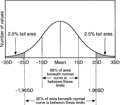
FIGURE 2.1 The normal (Gaussian) distribution. The normal range encompasses values falling between two standard deviations above and below the mean and includes approximately 95% of all the values.
‘Normal’ is a term used in statistics to describe a Gaussian distribution. Although the term ‘normal range’ is statistically valid only when the distribution is Gaussian, many analytes frequently measured in the laboratory have a skewed distribution – most frequently with a skew (tail) towards higher values. Examples include plasma alkaline phosphatase activity and the concentrations of triglycerides and bilirubin. A further drawback to the use of the term ‘normal range’ is that the word ‘normal’ has several different meanings in addition to its use in statistics. Given that the normal range, as defined above, encompasses only 95% of values characteristic of the chosen sample, 5% of individuals are bound to have values outside that range and might thus be considered ‘abnormal’. This is clearly absurd in relation to the more colloquial meanings of the word, for example ‘usual’, ‘acceptable’, ‘typical’ or ‘healthy’.
Often there is not a definite cut-off associated with an analyte, but a continuum of increasing risk with increasing concentration. An excellent example of this is the risk of coronary heart disease associated with increasing plasma cholesterol concentration, which extends below even the value of 5.0 mmol/L, often regarded as being an appropriate target for healthy (low risk) individuals. Indeed, although the curve of risk against cholesterol concentration becomes very shallow at low concentrations, it does not entirely flatten out (Fig. 2.2): that is, there is a continuum of increasing coronary risk associated with higher plasma cholesterol concentrations even in the lower part of the range of values typically found in adults in the UK. In this context, then, the term ‘normal range’ is potentially misleading: it is more relevant to define target values, which will depend on the overall level of coronary risk.
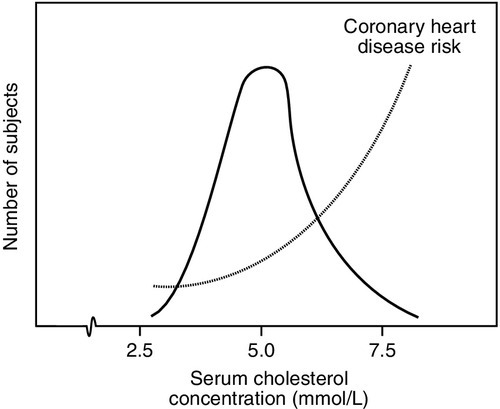
FIGURE 2.2 The distribution of serum cholesterol concentration in healthy subjects and risk of coronary heart disease. More than one-third of the values exceed the recommended highest acceptable concentration (5.0 mmol/L) and are associated with significantly increased risk. Note that the distribution is non-Gaussian, being skewed to the right.
Furthermore, even in patients with established disease, results may fall within the ‘normal range’. For most analytes, there is an overlap between the values usually encountered in health and those encountered in disease (particularly if the disturbance is mild). Thus, it should not be assumed that all patients with values within the normal range for a particular analyte are free of the relevant disease, just as it has been indicated that (by definition) not all patients with values falling outside the range are necessarily abnormal in any other way.
Reference values
Such considerations led to the development, in the late 1960s, of the concept of reference values. The word ‘reference’ is free of the ambiguities associated with ‘normal’. A reference value is defined as the value for an analyte obtained by measurement in an individual (reference individual) precisely selected using defined criteria, for example sex, age, state of health or other relevant characteristics.
The qualities required of a reference individual are only those specified: the term should not be taken as implying the possession of any quality (e.g. ‘healthiness’) that has not been specified. If measurements are made on a representative sample (reference sample) from a population of reference individuals (reference population) a distribution of values (a reference distribution) is obtained.
Reference limits can then be set and the range between these is defined as a reference interval. Typically, reference limits are set so that the interval encompasses values found in 95% of the reference samples, and this interval may then numerically be the same as the statistically defined normal range. Reference intervals are often colloquially termed ‘reference ranges’, but, strictly speaking, this is incorrect usage, since the true reference range encompasses the whole range of values derived from the reference population. The term ‘reference range’ is used in this book in accordance with common practice as a more familiar synonym for the term ‘reference interval’.
Reference values can be obtained by carrying out measurements on a carefully selected and precisely defined reference sample. If the distribution of values is Gaussian, the reference limits are the mean minus two standard deviations and the mean plus two standard deviations. When the distribution is non-Gaussian, the range can be calculated by ranking the values and deleting the lowest and highest 2.5%. Such a procedure has the considerable advantages that it requires no assumptions to be made about the characteristics of the distribution and does not require any transformation of the data to be made.
When the reference interval is derived from a sample of healthy individuals not known to be at increased risk of disease, the term effectively means ‘values characteristically found in a group of healthy individuals and thus likely to encompass values found in other, comparable (with regard to age, sex etc.) healthy individuals’. It is sometimes called a ‘health-associated reference interval’. Note, however, that health is not essential to the definition. Reference values could as well be established for analytes in disease as in health, although in practice this has not often been done (and, as indicated above, their ranges would almost always overlap with the corresponding health-related reference ranges).
Many strategies have been suggested for expressing observed values for biochemical variables in relation to the reference range: for example, the observed value can be expressed as a percentage of the mean of the reference interval or of the upper reference limit to give a ‘centi-normalized unit’. Most such suggestions have not been adopted in clinical practice. For enzyme measurements, however, where the values obtained can be highly method-dependent and can, in disease, be orders of magnitude higher than reference values, it is sometimes helpful to express results as multiples of the upper reference limit. Measurements used in antenatal screening, e.g. α-fetoprotein and human chorionic gonadotrophin, are often reported as ‘multiples of the median’.
An alternative suggestion has been to quote a ‘reference change value’, which looks at a patient’s usual intraindividual variation and expresses the observed value as a percentage of the mean individual reference interval. The development of sophisticated laboratory information systems has enabled alternatives to the reference range to become a realistic possibility.
Problems with reference intervals
Even reference intervals have disadvantages. However derived, they encompass the values from only 95% of the reference population. Thus, 5% of reference individuals will have values outside the reference limits. If two analytes that vary independently are measured, the probability of one of them being outside its reference limits is (1–0.952), that is 0.10. Of the reference individuals, 10% would be expected to have one of the measured values outside the reference limits. For ‘n’ analytes that vary independently, the probability is (1–0.95n), so that if 20 analytes were to be measured in an individual, there would be a 64% chance of one result being outside the reference limits. In practice, many tests are dependent on one another to some extent (e.g. total protein and albumin), so that this probability is reduced, but the calculation serves to emphasize that, even where values characteristic of health and disease have a completely bimodal distribution (i.e. non-overlapping ranges, something that happens very rarely in practice), by no means all observed results outside the health-related reference limits would be associated with disease. On the other hand, common sense dictates that the further away from the reference limit an observed result is, the more likely it is to be pathological in origin.
Comparison of observed results with reference limits
The importance of comparing observed results with appropriate (e.g. age- and sex-specific) reference intervals has already been emphasized.
As has been discussed, the appreciation of analytical and intrinsic biological variation for each analyte is also important. The implications for the interpretation of observed data on patients are considerable. As an example, we can consider the measurement of creatinine in plasma, widely used as a test of renal function. Its (health-related) reference interval is of the order of 60–110 μmol/L, but this does not mean that this range of values will be observed over time for a single healthy individual. The intraindividual biological variation of creatinine concentration is around 4.6 μmol/L so that the reference interval for individuals is approximately 18 μmol/L. Thus, two healthy individuals from the reference population might have typical creatinine concentrations that ranged between, for example 60–78 μmol/L and 85–103 μmol/L, respectively. But, as will be discussed in the next section, a change in plasma creatinine concentration in an individual from 70 to 98 μmol/L would almost certainly signify a decrease in renal function, even though both results are well within the population-based reference interval.
When (as is usual) there is overlap, or even a continuum, of values of an analyte in health and disease, it may be necessary to define a cut-off value to determine if further action should be taken (e.g. initiating further investigations). This is particularly true of screening tests, when there may be no other information to take into account in deciding the significance of a result. The considerations on which the selection of such a cut-off value depends are discussed later in this chapter.
In summary, it is important to appreciate that the information that can be provided by a single biochemical measurement is limited. In general, the results of complementary or serial measurements are often of much greater value.
Comparison of results with previous values
The problem posed in the interpretation of a test result when the test has been performed previously, is a different one. The relevant questions are, ‘Has there been a change and, if so, is it clinically significant?’.
In order to assess the relevance of any change to a pathological process, it is necessary to have a quantitative indication of the possible contribution of analytical and intrinsic biological variation to the observed change. The probability that a difference between two results (whether an increase or a decrease) is significant at the 95% level (i.e. that such a difference would only be expected to occur by chance alone on fewer than one in 20 occasions), requires that the difference is 2.8 times the variation (SD) of the test (for the basis of this calculation, see Fraser 2001, in Further reading, below). Because of the contribution of both analytical and biological variation, the standard deviation of the test is given by:
where SDA is the analytical variation and SDB is the biological variation. One set of estimates of the value of 2.8 × SD, also known as the critical difference (more formally called the ‘reference change value’), for some frequently measured analytes, is given in Table 2.5. These values appear to differ little in health and disease and are valuable guides to clinical decision-making. Two caveats are important. First, the values quoted are mean values: individuals may show greater or lesser intrinsic biological variation. Second, analytical performance (and hence analytical variation) varies considerably between laboratories: ideally, laboratories should calculate their own values for critical differences, although in practice, this is seldom done.
TABLE 2.5
Critical differences: changes required in the plasma level of some frequently measured analytes to be of significance in an individual
Data from various sources, including UKNEQAS (UK National External Quality Assurance Scheme) website and Ricos et al. on Westgard QC website (see Further reading).
It should be emphasized that, just because a change in the level of a biochemical variable exceeds the critical difference calculated from the known biological and analytical variation, it does not necessarily follow that it is clinically significant: that will depend on the precise clinical circumstances and needs to be assessed in relation to whatever clinical and other data are available. For example, restriction of dietary protein intake may cause a considerable reduction of plasma urea concentration in a patient with chronic renal disease, but this does not signify an improvement in renal function. The reverse is also true: the lack of a change does not necessarily imply that there is no cause for concern. For example, the haemoglobin concentration of blood may initially remain within health-related reference limits for a short period, even after severe acute bleeding, because erythrocytes and plasma have been lost together.
Another important point in relation to critical difference values, is a possible difference between laboratory staff and clinical staff in ascribing significance to an apparent change. The choice of a probability of 0.95 that two results are significantly different is arbitrary, although hallowed by practice. A probability of 0.99 is clearly more significant, but if two results differ with a probability of only 0.9, there is still a 9 in 10 chance that they are truly different. Decisions in medicine are still frequently made on much lower probabilities. It would be feasible to construct lists of critical differences at different levels of probabilities, but to publish such lists in laboratory handbooks would make them cumbersome and potentially confusing. However, laboratories should be able to provide guidance in this area to recently qualified clinicians and for newly introduced investigations.
In practice, critical values for difference used by clinicians are often empirical and not based on any formal assessment. This does not invalidate their use; indeed, they have often been validated informally by long experience and observation of outcomes. However, they fall short of the requirements of ‘evidence-based clinical biochemistry’ (discussed in Chapter 3).
Most instrument-based or laboratory-based management systems incorporate automatic procedures for identifying large (and potentially significant) changes in biochemical variables (‘delta checks’). Despite every effort to reduce analytical variation, such changes may arise because of unusual analytical imprecision or random error. Gross analytical errors (‘fliers’) will often be obvious because they are greater than typically occurs clinically. Smaller errors may not be obvious. Deciding whether a change in a variable is likely to represent a real change in the patient requires checks on the identity of the specimen, internal quality control performance and the clinical details, if these are available on the request form or can be deduced from other information (the patient being located in the intensive therapy unit, for example), all of which the clinical biochemist will use in deciding what action to take. If the identity of the specimen is confirmed, the assay run was in control and the change is consistent with what is known about the patient, the result can be reported; if not, the original specimen may need to be re-analysed or a further specimen obtained from the patient.
As well as ‘delta checks’, laboratories should be able to identify action limits, such that unexpectedly high or low results that may require an immediate change of management (e.g. low or very high serum potassium concentrations) are checked and communicated rapidly to the requesting clinician. Specific values may be set to trigger further investigations on the basis of protocols agreed with the appropriate clinicians, for example magnesium if the corrected calcium concentration is low, or serum protein electrophoresis if the total globulin concentration is increased. All these procedures are of potential value to the patient and add to the clinical usefulness of the results in question.
THE PREDICTIVE VALUE OF TESTS
Introduction
It will have become clear that the interpretation of biochemical data is bedevilled by the inevitable presence of analytical and intrinsic biological variation. It is still frequently assumed that a result within reference limits indicates freedom from disease or risk thereof, while a result outside reference limits at least requires that the patient be further investigated. What is lacking is any numerical indication of the probability that a particular result indicates the presence or absence of disease.
The predictive value concept, introduced into clinical biochemistry in the mid-1970s by Galen and Gambino, represents an attempt to address these shortcomings. Essential to the concept of predictive values is that disease or freedom from disease can be defined absolutely, that is, that there is a test which can be regarded as the ‘gold standard’. For some conditions, this will be histological examination of tissue obtained at surgery or post-mortem, but it may be the eventual clinical outcome or some other more or less well-defined endpoint. It is against the gold standard that biochemical tests may be judged.
Definitions
If all the members of a population consisting of people with and without a particular disease are subjected to a particular test, the result for each of them will fall into one of four categories:
• true positives (TP) – individuals with disease, who test positive
• false positives (FP) – individuals free of disease, who test positive
• true negatives (TN) – individuals free of disease, who test negative
• false negatives (FN) – individuals with disease, who test negative.
Clearly, the number of individuals with disease equals (TP + FN) and the number without equals (TN + FP). The total number of positive tests is (TP + FP) and of negative (TN + FN).
These data can conveniently be arranged in a matrix (Table. 2.6). It is then easy to derive the other important parameters relating to test performance, that is, prevalence, sensitivity, specificity, predictive value and efficiency (Table 2.7).

TABLE 2.7
Important parameters relating to test performance
| Parameter | Definition | Formula (expressed as %) |
| Prevalence | Number of individuals with the disease expressed as a fraction of the population | TP + FN/ (TP + FN + TN + FP) |
| Sensitivity | Number of true positives in all individuals with disease | TP/(TP + FN) |
| Specificity | Number of true negatives in all individuals free of the disease | TN/(TN + FP) |
| Positive predictive value | Number of individuals correctly defined as having disease | TP/(TP + FP) |
| Negative predictive value | Number of individuals correctly defined as free from disease | TN/(TN + FN) |
| Efficiency of test | Fraction of individuals correctly assigned as either having, or being free from disease | (TN + TF)/(TP + TF + FP + FN) |
TP = true positive; TN = true negative; FP = false positive; FN = false negative.
The predictive value model examines the performance of a test in defined circumstances. Clearly, it depends upon being able to determine the numbers of true and false positive and negative results, which depends upon there being an independent, definitive diagnostic test. The importance of the independence of the test under investigation from the definitive test may appear self-evident but, in practice, it is frequently overlooked.
Example
These concepts, and some of the pitfalls inherent in their use, can be illustrated with reference to a hypothetical example. Suppose that it is desired to assess the value of measurements of serum γ-glutamyltransferase activity to assist in the diagnosis of alcohol abuse in patients attending a drug-dependency clinic. It is decided that the test will be regarded as positive if the γ-glutamyltransferase activity exceeds the upper reference limit. Disease status is determined by a validated questionnaire.
Over the course of a year, 200 patients are tested. Enzyme activity is found to exceed the chosen limit in 73, but only 62 are judged to be abusing alcohol on the basis of the rigorous questionnaire. In 18 individuals judged to be abusing alcohol, enzyme activity is not elevated.
The results matrix can thus be completed as in Table 2.8. Calculation then shows that:

Prevalence = (62 + 18)/200 = 0.400 = 40%
Sensitivity = 62/(62 + 18) = 0.775 = 78%
Specificity = 109/(109 + 11) = 0.908 = 91%
PV(+) = 62/(62 + 11) = 0.849 = 85%
PV(−) = 109/(109 + 18) = 0.858 = 86%
Efficiency = (62 + 109)/200 = 0.855 = 86%
Thus, the test correctly identifies 78% of alcohol abusers; further, if a patient has an elevated enzyme activity, there is an 85% probability that he is abusing alcohol. However, it might be considered that a significant number of patients are being misclassified and that better performance might be achieved if the cut-off value for a positive test were to be set at a higher enzyme activity, say twice the upper reference limit.
The results matrix might then appear as in Table 2.9, from which:

Prevalence = (50 + 30)/200 = 0.400 = 40%
Sensitivity = 50/(50 + 30) = 0.625 = 63%
Specificity = 118/(118 + 2) = 0.983 = 98%
PV(+) = 50/(50 + 2) = 0.961 = 96%
PV(−) = 118 (118 + 30) = 0.797 = 80%
Efficiency = (50 + 118)/200 = 0.840 = 84%
The effect has been to decrease the sensitivity of the test, which now only correctly identifies 63% of alcohol abusers. On the other hand, if a patient tests positive, the probability that he is an alcohol abuser is now 96%. The overall efficiency of the test is little changed.
This example illustrates two important points about the predictive value model. The first is that sensitivity and specificity tend to vary inversely; second, appropriate selection of the criterion for positivity or negativity (here the level of enzyme activity) allows either one to be maximized. If the cut-off is set very high, positive results will only occur in individuals with disease; there will be no false positives and specificity will be 100%, although sensitivity will be low. On the other hand, if the cut-off is set low, no cases will be missed, but the false positive rate will be high; sensitivity will be 100%, but specificity will be low. This is illustrated in Figure 2.3.
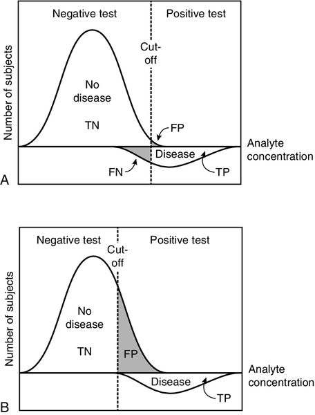
FIGURE 2.3 The effect of moving the cut-off point that determines positivity/negativity of a test result. Hypothetical distributions for the concentrations of an analyte with and without disease are shown. Because these overlap, if the cut-off is selected to decrease the number of false positive (FP) results (and hence increase specificity), (A) there are a significant number of false negative (FN) results (decreasing the sensitivity). If the cut-off is set lower (B), false negatives are eliminated (maximizing sensitivity), but at the expense of increasing the number of false positives (and decreasing specificity). The distribution for individuals with disease has been shown below the axis for clarity. TP, true positive; TN, true negative.
Whether it is desirable to maximize sensitivity, specificity or efficiency depends on the nature of the condition being investigated, as discussed below.
Prevalence and predictive value
While sensitivity and specificity are dependent on the characteristics of the test and the nature of the condition being investigated, predictive values are dependent on the prevalence of the condition in the population under examination. Consider the application of the measurement of γ-glutamyltransferase activity to identify alcohol abuse during pregnancy. If 500 women were screened and the cut-off taken as the upper limit of the reference range, then the results matrix might show as in Table 2.10, from which:

Prevalence = (24 + 7)/500 = 0.062 = 6%
Sensitivity = 24/(24 + 7) = 0.774 = 77%
Specificity = 426/(426 + 43) = 0.908 = 91%
PV(+) = 24/(24 + 43) = 0.358 = 36%
PV(−) = 426/(426 + 7) = 0.983 = 98%
Efficiency = (426 + 24)/500 = 0.900 = 90%
The sensitivity and specificity are unchanged compared with the previous example, but, because of the much lower prevalence of alcohol abuse in this group, the predictive value of a positive test is low: only 36% of those with a positive test are alcohol abusers. At the same time, the predictive value of a negative test is higher than in the patients attending the drug dependency clinic: this is again a consequence of the lower prevalence in pregnant women. It is instructive to note that the efficiency of the test appears greater in this context (90% in comparison to 84% in the drug abuse patients). Overall, the proportion of tests that correctly assign patients to the alcohol abuse or non-abuse categories is higher, although its performance in diagnosing abuse alone is poorer.
The effect of disease prevalence on predictive values is an important one. It means that the performance of a test in one group of patients cannot be translated to a different group. Although the predictive value of a new test may appear high in the typical experimental setting where equal numbers with and without disease are tested (the prevalence is 50%), it is likely to be much lower ‘in the field’. Thus, the performance of a new test must be analysed in groups of individuals comparable with those in whom it is to be used in practice. In the past, many exaggerated claims for tests have been made on the basis of their performance in a highly selected group.
Practical applications of the predictive value model
High sensitivity in a diagnostic test is required when a test is being used to diagnose a serious and treatable condition. The false negative rate (missed diagnoses) must be as low as possible, even though this inevitably means that false positives will occur. Individuals testing positive will be subjected to further, definitive tests and, provided that these cause no harm to those who test positive and turn out not to have the condition, this may be an acceptable price to pay for making the diagnosis in all those who have the condition. The programmes for neonatal screening for phenylketonuria and other harmful conditions in the newborn exemplify tests requiring maximum sensitivity. In this context, it is instructive to note that although the sensitivity of the screening test for phenylketonuria is 100%, and its specificity approaches this value, because the condition has such a low prevalence (approximately 1 in 10 000), the predictive value of a positive test is only of the order of 10%.
High specificity (no false positives) is desirable in a test to diagnose a condition that is severe, but either it is untreatable or the benefits of treatment are unpredictable, when knowledge of its absence is potentially beneficial. Multiple sclerosis is frequently cited as the classic example of such a condition. High specificity is also required when it is desired to select patients with a condition for a trial of some new form of treatment. If individuals without the condition were to be included in the treatment group, the results of the trial (assuming that the treatment is in some measure effective and does no harm to those without the disease) would give a false view of its efficacy.
Diagnoses are rarely made on the basis of single tests. Ideally, a single test or combination of a small number of tests should be used to identify individuals in whom the probability of a condition is significantly higher than in the general population (the prevalence is higher), who can then be further investigated. The initial tests can be simple, cheap and unlikely to do harm, but the further tests may be more elaborate, expensive and possibly associated with some risk. In essence, if the performance of individual tests is known and the objectives of testing can be precisely defined, the predictive value model can be used to determine the appropriate sequence or combination of tests to achieve the desired objective.
Receiver operating characteristic curves
Another use of the predictive value model is to compare the performance of two tests. This can be done by determining sensitivity and specificity for each test using a range of cut-off limits to define positivity and plotting one rate against the other. The resulting curves are known as receiver operating characteristic (ROC) curves. The reader is warned that four variants of ROC curves may be encountered, according to the way the data are projected on the axes, but this does not affect their interpretation. Figure 2.4 shows hypothetical ROCs for two tests, A and B, each applied to the same group of individuals to make the same diagnosis.
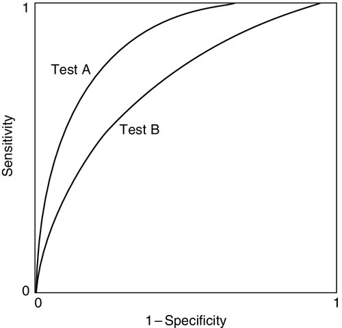
FIGURE 2.4 Receiver operating characteristic curves for two tests being assessed for the diagnosis of the same condition in the same patients. Test A gives better specificity at any level of sensitivity.
It is clear that test A gives the better discrimination, since for any level of sensitivity its specificity is superior. This may be useful information, but these are by no means the only factors that may need to be taken into account in choosing a test. The economics and practicalities of the tests will also be of relevance to which one is chosen.
The interpretation of the ROC curves in Figure 2.4 is straightforward. In practice, the curves for two tests may cross; the relative performance must then include assessment of the areas under the curves. The greater the area, the greater the efficiency.
Likelihood ratios
Although the predictive value model can be used to determine the most appropriate cut-off for a test result for clinical purposes, it can only classify results as positive or negative, and does not give any indication of the degree of abnormality, which may be of prognostic significance.
In contrast, likelihood ratios can be applied to individual test results. The likelihood ratio states how much more likely a particular test result (or combination of results) is to occur in an individual with a disease than without it (positive likelihood ratio, LR(+)), or not to occur, again in individuals with a disease than without it (negative likelihood ratio LR(−)). The ratios are calculated thus:
LR(+) = sensitivity/(1 − specificity)
LR(−) = (1 − sensitivity)/specificity.
To give an example, an LR(+) of 10 implies that the given result will be obtained ten times more frequently in a population with the condition in question than in one without. A LR(−) of 0.01 implies that the given result will be obtained 100 times more often in individuals without the condition than in those who have it. Calculation of the LR(+) and LR(−) allows the post-test probabilities for either a positive or negative result to be calculated. The post-test probability can be calculated as follows:
The pre-test probability is equal to the prevalence of the condition in comparable individuals (e.g. a population being screened).
Positive and negative likelihood ratios can be combined to give the diagnostic odds ratio (DOR) for a particular test result:

The DOR expresses the odds of a result being positive in a patient with the condition being investigated compared with one who does not have the condition, and is a measure of the overall accuracy of a test.
CONCLUSION
It is a simple matter to fill out a request form for a biochemical test, but before doing so, it is essential to consider why the test is being done and for what the results will be used. Many factors can affect the results of laboratory tests, apart from the pathological process that is being investigated. Some of these are obvious, others less so. All need to be minimized by careful patient preparation, sample collection and handling, analytical procedures and data processing, if the results are to be reliable and fit for whatever purpose they are to be used.
The interpretation of biochemical data requires adequate knowledge of all the factors that can affect the test result. These include the physiological, biochemical and pathological principles on which the test is based, as well as the reliability of the analysis. It is also necessary to understand the statistical principles that relate to the distribution of data in healthy individuals and those with disease, and how the test performs in the specific circumstances in which it is used. Such knowledge is also essential for the appropriate selection of laboratory investigations.
ACKNOWLEDGEMENT
We would like to thank William Marshall, who wrote this chapter for previous editions of the book.
Further reading
Ricos C, Alvarez V, Cava F. Essay: biologic variation and desirable specifications for QC, http://www.westgard.com/guest17.htm.
A comprehensive list of data on biological variation and related matters, based upon the original article.
Swinscow TDV. Statistics at square one. 9th ed. 1997. Available for free online at: http://www.bmj.com/about-bmj/resources-readers/publications/statistics-square-one.
An excellent statistics book that begins from first principles.
United Kingdom National External Quality Assessment Service (UK National External Quality Assurance Scheme), http://www.ukneqas.org.uk/content/PageServer.asp?S=995262012&C=1252&CID=1&type=G.