Chapter 22
Computed Tomography
Jan D. Blankensteijn, Leo J. Schultze Kool
Conventional contrast-enhanced arteriography is no longer considered the standard imaging modality for vascular disease.1–6 As with many technologic advances, however, the process of image creation continues to become more difficult for the average end user to understand. Although the typical vascular surgeon can perform clinical evaluation and make decisions without an understanding of the basic principles behind computed tomography (CT), these concepts remain important. A better grasp of the image creation process and terminology also aids collaboration between the radiologists creating the images and the surgeons who use the images to plan surgical interventions. Finally, an understanding of the basic concepts enhances the ability of the surgeon to understand technologic advances as they become the new standard of care.
Basic Principles
In the early 1930s, the Dutch radiologist Ziedses des Plantes first devised a technique that reduced the problem of superimposition of structures in basic radiography (x-ray tube and plain film). Physically connecting the x-ray tube and film opposite each other and rotating the combination around a body segment sharpens the image created by the points on the focal plane, whereas the images of points outside the focal plane are blurred, thereby creating less superimposition artifact. This technique was called “planigraphy” or “tomography,” derived from the Greek words tomos, which means “a section” or “a cutting,” and graphein, meaning “to write.” Tomography played an important role in diagnostic radiology until the 1970s, when invention of the transverse axial scanning method together with the availability of minicomputers, which allowed computational reconstruction of images, led to the development of so-called computed axial tomography (CAT scan, or later CT scan).
Two similar methods for transverse axial scanning and image reconstruction were independently invented by Sir Godfrey Newbold Hounsfield in Hayes, United Kingdom, at Elector-Musical Instruments (EMI) Limited Central Research Laboratories, and Allan McLeod Cormack of Tufts University in Massachusetts. A combination of hardware, mathematical algorithms, and computer software resulted in the cross-sectional images. The first so-called EMI scanner was installed in Atkinson Morley’s Hospital, Wimbledon, England, in 1971.7 In the United States, the first installation was at the Mayo Clinic in Rochester, Minnesota. These machines would acquire two adjacent brain tomographic sections in about 4 minutes and needed about 7 minutes of computation time per picture. This was such a leap forward in imaging technology that Hounsfield and Cormack shared the Nobel Prize in 1980.
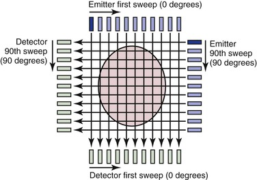
Many of the principles used in this first-generation CT scanner are still in use today and provide a framework for understanding the technology. The fundamental unit for this scanning method consists of an emitter and a detector; an x-ray beam is transmitted through the tissue and detected on the other side. The emitter produces a thin (highly collimated) x-ray beam that sweeps in linear fashion across the body cross-section (Fig. 22-1). The detector moves as a unit with the emitter and records data from 160 separate, parallel, and immediately adjacent beams. The emitter and detector units are mounted within a gantry, which is rotated 1 degree before another linear, transverse sweep takes place. This process is repeated through 180 degrees of rotation to produce the data necessary to form a 160 × 160 matrix for a single cross-sectional image. The attenuation (the rate of reduction of x-ray energy recorded at the detector) of multiple x-ray beams traversing the same point in the matrix from different angles is collected and an ingenious method applied to calculate backward to the density or CT number that must be present at each location in the matrix.
The resulting CT number is said to be expressed in Hounsfield units (H). Clinically, CT numbers range from the extremes of air (−1000 H) to dense bone (>1000 H), but fat (−20 to −100 H), water (0 H), and muscle and blood (40 to 60 H) tend to lie in a much narrower range. Differences in factors such as the energy level of the beam and tissue thickness prevent the density in Hounsfield units from being absolutely uniform from one CT scan to another, but the ranges are similar. When the range of CT numbers for a scan is determined, it can be broken up into smaller ranges for graphic display by a set of gray-scale values. In the chest, CT numbers approaching 1000 H (bone) are typically assigned values close to pure white, whereas CT numbers approaching −1000 H (air) are typically assigned values close to pure black. CT numbers between −1000 and +1000 H would be displayed as graduated shades of gray. Each gray-scale data point in the matrix is known as a pixel because it represents a “picture element.” When displayed as a whole, this matrix of gray squares becomes an interpretable image.
Types of Scanners
Single-Slice Sequential CT
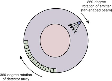
A first-generation CT scanner is capable of producing a cross-sectional image with a 160 × 160 matrix. These CT scans were applicable only to parts of the body with limited motion (e.g., the head) because the back-calculation algorithm depends on the subject’s remaining in one position while data are collected for the entire cross-section. To obtain useful scans in areas such as the chest and abdomen, subsequent generations of CT scanners were designed to decrease the time required to obtain a complete cross-sectional image. The second-generation CT scan used an emitter that produced a broader fan-shaped x-ray beam and an array of 30 detectors instead of a single detector. These innovations greatly reduced the number of emitter locations required to complete a single transverse sweep, as well as the number of transverse sweeps (1-degree increments were no longer required for a complete cross-sectional image). The time for a single cross-sectional scan was reduced to approximately 15 seconds. In a third-generation scanner, the emitter produces a wider fan-shaped x-ray beam, and hundreds of detectors are arranged in an arc (Fig. 22-2). Because the beam/detector combinations cover the entire patient, no transverse sweep is required—the emitter and detector array rotate in a continuous 180- or 360-degree arc to produce a complete cross-sectional scan in 1 second. In a fourth-generation CT scanner, the detector array covers the entire 360-degree arc and only the emitter rotates.
Spiral (Helical) CT
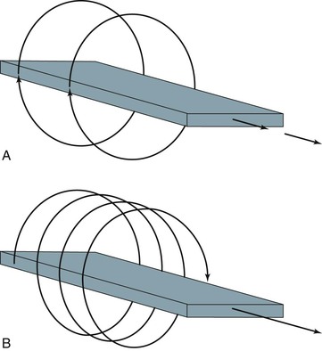
With development of the slip-ring gantry, the emitter and detector array can rotate continuously in the same direction, and at the same time, the computer can acquire data continuously. With conventional CT, there would still be a pause in data acquisition while the table (patient) moves to a new position for the next cross-section to be scanned. If the table moves in a continuous linear motion through the gantry while the x-ray emitter and detector rotate continuously over 360 degrees, data can be acquired in a single sweep over the entire volume of interest. In this technique the emitter traces out a spiral relative to the patient, which is referred to as a spiral CT or helical CT scan (Fig. 22-3).
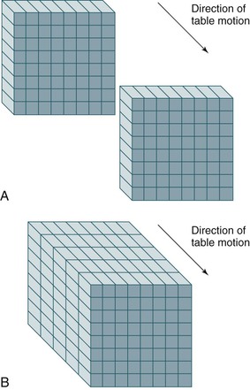
Spiral or helical CT technology has several important ramifications beyond a simple decrease in scan time. A spiral CT scan collects data over a continuous volume rather than discontinuous slices (Fig. 22-4). The most obvious advantage of acquiring data over a continuous volume is that thin axial slices can be reconstructed from the digital data set at arbitrarily small intervals without additional radiation exposure. Single-slice sequential CT can produce similar overlapping or adjacent axial slices, but the tradeoff is increased scan time and additional radiation exposure. The advantage of sequential scanning, however, is a lower level of reconstruction artifacts because table movement along the z-axis during scanning does not need to be corrected in the acquired data sets. This is the main reason why sequential scanning is often used for brain imaging.
Multislice (Multidetector) CT
Multidetector scanners have multiple rows of detectors, so that the volume to be scanned can be covered more quickly. Whereas a single-slice detector acquires one slice per rotation, multidetector CT scanners are capable of acquiring multiple separate slices. Each slice can be acquired at 1-mm or even submillimeter thickness with rotation times in the range of subseconds. Complete imaging of the abdominal vasculature can be accomplished in a fraction of the time required with previous-generation scanners, which can diminish or eliminate many artifacts or compromises that must be dealt with in single-row detector scanners, as discussed subsequently. For this reason, multidetector or multirow scanners have almost completely replaced the earlier-generation single-row scanners.
Advances in hardware and computer software technology have also greatly improved the graphic image display despite the reduction in scan times. A first-generation CT scanner produced a cross-sectional image with a 160 × 160 matrix, but current scanners typically generate a 512 × 512 matrix. Each data point in the matrix is mapped to a gray scale for display, so the size of the matrix and the field of view (FOV) have a direct impact on resolution of the display (the smallest distinguishable element). Data points are displayed as a two-dimensional (2D) picture, and each point in the display matrix is a pixel (picture element). Data points are acquired in three dimensions, however, and each data point in the matrix actually represents a voxel (volume element). The size of the voxel is determined by multiple factors, including detector design, FOV (x, y direction), and thickness of the x-ray beam (z direction). One current advantage of CT over magnetic resonance imaging (MRI) is that CT is typically displayed in a 512 × 512 or greater matrix, with resolution of 0.2 to 1 mm2 for each pixel. MRI is generally limited to a 256 × 256 matrix, and resolution in the axial plane is roughly half that of CT.
CT Angiography
Visualization of vessels on CT is limited by the similar densities of blood and soft tissue. Although administration of intravenous contrast material can overcome this problem to some extent, optimal visualization of the vessels (computed tomographic angiography [CTA]) was not possible until the availability of spiral CT. The main advantage of spiral CT over sequential CT is the possibility of imaging a larger part of the body in a shorter time. Such fast scanning allows visualization of the vessels during the short period that a bolus of contrast material passes the imaged volume. Thus faster scan times and increased numbers of detectors will allow a larger part of the body to be imaged as the contrast bolus passes.
Timing of the initiation of image acquisition relative to injection of the contrast agent is crucial for maximizing opacification of vessels in the scanned volume. Various dedicated algorithms have been developed by the CT scanner manufacturers, but they are all based on a stationary, continuous scan of a single slice in which contrast density is measured in an area of interest (usually a large vessel) marked by the operator. Only after a sufficient increase in density is measured is the spiral CT run initiated.
Both the length and the density of the contrast bolus are important parameters. Bolus length should be balanced against the length of the volume to be imaged. Because large distances must often be covered, CTA generally requires a significant infusion of contrast material. In the past, a typical CTA study from the celiac axis down to the external iliac arteries would require 120 to 180 mL of 300 mg/mL nonionic contrast.8,9 Optimization of scanning and power injector protocols and the use of saline push bolus techniques reduced this volume significantly, and often volumes do not exceed 100 mL.
Acquisition Parameters
All the concepts and considerations mentioned previously are ultimately used to form a scan protocol. A scan protocol consists of a series of settings of acquisition and contrast parameters, reconstruction parameters, technician and patient instructions, and maneuvers to generate a set of images that is optimal for the specific anatomy and indication for the CT scan. The protocol includes the setting of x-ray emitter parameters (i.e., kilovolts peak [kVp] and milliampere-second [mAs]), length of helical exposure, pitch, collimation, patient instructions (i.e., breath-hold), dosage of contrast material, delay, volume and infusion rates, reconstruction interval and algorithm, parameters of radiation dose optimization tools, and FOV.
Prescan and postscan parameter settings should be distinguished. Various postscan settings, such as the reconstruction algorithm or interval, can be applied to the raw image data. This is not true for the prescan settings. Obviously, an improper prescan setting cannot be corrected after the images have been acquired. Particularly in multislice scanners, proper prescan settings are important and have a direct impact on the diagnostic value of the scan.
Scan parameter settings are also important for optimization of the scan protocol in relation to the clinical question because this may be the only way to limit the radiation dose delivered by the scan.
Prescan Parameters
kVp and mAs.
Tube voltage, measured in kVp, is the value that determines the energy level of the x-ray tube. Higher tube voltage renders better tissue penetration but leads to decreasing relative contrast differences between the various tissues. High kVp settings (120-140) are recommended to allow sufficient photons to reach the detector elements in obese patients but also in regions with high x-ray attenuation (shoulders, abdomen, pelvis). In children or slim patients, low kVp settings (80) should suffice and also produce increased contrast differences.
mAs values describe the tube current time product. The mAs value is linearly related to the duration and amount of radiation. Higher mAs represents more radiation delivered by the x-ray tube and leads to a decrease in image noise because more photons will reach the detector. However, this decreased noise is achieved at the expense of an increased radiation dose to the patient. kVp and mAs settings are closely linked, and a change in one may dictate a change in the other.
Collimation.
Collimation is a method of reducing the thickness of the x-ray beam. Collimation has a direct impact on spatial resolution in the z-axis and determines the smallest possible slice thickness (postscan parameter).
Table Feed and Pitch.
Pitch (P) is defined as the ratio of table feed (the speed at which the table moves during tube rotation) and collimation. Values above 2 will result in undersampling of the region of interest and might result in artifacts. Values below 1 will result in overlapping scans, which might be beneficial for three-dimensional (3D) reconstructions but will also increase the dose significantly if other scanning parameters are kept constant. For multislice CT scanners, pitch calculations are different, depending on whether single collimation of one detector ring or total collimation of the whole detector array is chosen. An asterisk indicates that total collimation of the detector array is being described; for a four-slice scanner, a pitch of 2 corresponds to a P* of 8.


where P = pitch, TF = table feed, N = number of detectors, and SC = single-section collimation.
To give an example for a 64-slice scanner, if pitch is set at 2 and collimation is set at 1 mm, the resulting TF—according to the formula P*= TF/(N × SC)—will be 64 mm/sec.
Scanning time is the maximum duration of a scan that a certain tube allows while not exceeding the maximum permissible heat capacity. Older scanners are limited to approximately 20 seconds, whereas newer scanners allow scan times of up to 100 seconds.
Patient Positioning.
Proper positioning of the patient can significantly improve image quality and decrease radiation dose. A clear example is raising the arms of the patient when scanning the upper part of the chest (Fig. 22-5).
Contrast Protocols.
With the newer scanner types, good timing of the administration of contrast material has become an essential part of the examination. Depending on the indication and parameter settings (pitch), optimization of total volume of contrast, contrast iodine density, volume, and speed of injection is required.
Postscan Parameters
Increment.
The increment or reconstruction index defines the spacing of the reconstructed images from the raw data set. One could, for instance, decide to reconstruct only a 1-mm slice every 3 mm. The main advantage would be the fewer number of reconstructed slices than if a 1-mm slice had been reconstructed for every position. If the raw data are saved, it is possible to obtain reconstructed images at different positions retrospectively.
Slice Width.
Slice width or section collimation defines the thickness of the slice. Slices of various thickness ranging from 0.5 to 10 mm can be calculated from the raw data. The minimum slice thickness, however, is defined by the prescan collimation setting. The main advantage of a thicker slice is a lower noise level and a significant reduction in the data load produced by modern multislice scanners.
Field of View.
As mentioned previously, the size of the display matrix and FOV have a direct impact on axial resolution of the display. By keeping FOV to the minimum necessary, pixel size is decreased. If FOV is 30 cm and the matrix size is 512 × 512, each pixel in the display of axial slices is 0.6 mm. If FOV is reduced to 20 cm, pixel size is improved to 0.4 mm, but the tradeoff is that a higher radiation dose is required because of an increase in detector noise.
In general, a small FOV is important only when detailed measurements are necessary (e.g., in endovascular surgery, calculation of carotid artery stenosis or intracerebral aneurysms). In addition, factors such as contrast density, timing of administration of contrast material, window level, and window width more strongly affect the ability to distinguish different structures and the edges of these structures (see Post Hoc Image Optimization discussion later in this chapter).
Windowing.
Window width (WW) sets the number of gray scales displayed, and window level (WL) defines the middle gray-scale value of the width. Windowing sets the contrast and the brightness of the image.
Reconstruction Algorithms.
Reconstruction algorithms (convolution kernel) are used to reconstruct the raw data. Because these algorithms determine the relationship between spatial resolution and noise and thus contrast resolution, different algorithms can be selected for different indications. If high spatial resolution (bone pathology) is needed, high-resolution convolution kernels are applied (HR kernels). With this algorithm a significant increase in spatial resolution is obtained, but it is achieved at the expense of a significant increase in image noise.
Dynamic CT Scanning
With the increased number of detector rings in the new multislice scanners, dynamic CT scanning has become an option.10 The basic concept is that of obtaining CT images at a fixed location (in other words, without moving the table) during the injection of contrast material. After injection of a contrast agent, imaging at a fixed position with continuous rotation of the CT gantry will provide insight into passage of contrast material through the arterial, capillary, and venous phases, representing tissue perfusion. The anatomic area covered by this type of imaging is determined by the length of the detector area. The 256 and 320 scanners are better suited for this technique and are currently used predominantly for brain and cardiac perfusion studies.
Retrospective electrocardiogram (ECG)–gated CT acquisition is a scanning technique in which the ECG is registered during the scan and coupled to the raw data obtained.11 By partial reconstruction of the images, it is possible to obtain an image at, for instance, eight different phases of the ECG. The technique is now available on almost all 64-slice scanners and is most often used for coronary imaging.12 Because partial reconstructions are used, a major drawback of this technique is that the resulting images are substantially noisier than the full reconstructions. In prospective ECG-gated CT acquisition, the x-ray beams are turned on during preselected phases of the cardiac cycle. The main benefit of this way of sampling is the lower radiation dose, which, in comparison with retrospective gating, proved to be reduced by 52% to 85%. The main disadvantage is that only preselected phases can be reconstructed.
Postprocessing
Multiplanar Reformatting
Another advantage of data acquisition over an entire volume is the ability to reconstruct or reformat the data in arbitrary planes. Reformatting CT data into coronal, sagittal, or other nonaxial planes is often referred to as multiplanar reformatting or multiplanar reconstruction (MPR). A schematic representation of this process is shown in Figure 22-6. The ability of spiral CT to view the data in coronal, sagittal, or arbitrarily defined planes often gives more insight into vascular anatomy than possible with axial views alone.13
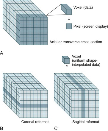
Figure 22-6 A-C, Because spiral CT data are acquired and stored over a continuous volume, they can be used to create axial (A), coronal (B), and sagittal (C) sections. For display purposes, the nonuniform voxel can be interpolated into a cube, but the quality of the data still depends on the length of the original voxel (which is determined by the collimation). Reformatting CT data into coronal, sagittal, or other nonaxial planes is often referred to as multiplanar reformatting.
Measurements
Simple axial CT slices often do not cut through planes perpendicular to the vessel, which results in elliptical cross-sections that can make measurements of diameter difficult (Fig. 22-7). Generally, the narrowest diameter of the elliptical cross-section is the “true” arterial diameter, but this is not always the case because the aorta does not always have a simple cylindrical or conical shape.14 Conventional CT may lead to a slight overestimation of diameter on axial slices, whereas spiral CT slices reconstructed perpendicular to the vessel tend to be more accurate.3,15–18 Simply using sagittal or coronal reconstruction is not always adequate because these sections may not be perpendicular to the vessel or may not cut through the center of the vessel over an adequate length. Curvilinear reformats continue to improve, but they make measurements of length difficult and straighten out angles, which may affect an endovascular repair. Spiral CT with 3D reconstruction and CT reformats perpendicular to the vessel lumen eliminate the diameter measurement problems associated with the other techniques (see Fig. 22-7).3,15–18 CTA with 3D reconstruction offers several other important benefits that are key for imaging before endovascular surgery. In conjunction with spiral CTA and multiplanar reconstruction, 3D reconstruction speeds assimilation of the CT data and makes the extent of an aneurysm rapidly apparent.3,16,17 More important, specialized measurement software and unique aspects of the 3D reconstruction can eliminate most of the measurement problems associated with conventional techniques.3,15–18 Software algorithms can be used to display the centerline of the blood flow channel in the infrarenal aorta and iliac arteries and allow measurements of length along the vessel centerline in tortuous aortic or iliac segments.15 In some systems, graft paths along a line other than the centerline can be also defined by the user, which is necessary because an endovascular graft may not follow the centerline of the blood flow channel throughout its entire course.

Figure 22-7 Diameter measurement issues and solutions using CT. A, Three-dimensional (3D) reconstruction with simultaneous display of CT slices in 3D space. The CT slices shown here are a standard axial reformat and a reformat perpendicular to the aorta. The 3D model was rotated to show the intersection of the two CT slices at the same location on the aorta. B, The same axial CT slice as shown in A. The axial slice does not intersect the aortic neck perpendicular to its axis, thereby creating an elliptical cross-section. Although the smaller diameter (minor axis of the ellipse) is usually similar to the true diameter, elliptical cross-sections also occur in noncylindrical vessels and at the margins of aneurysms. Viewing multiple cross-sections in sequence can help with this problem, but evaluation is still difficult. C, The CT slice reformatted perpendicular to the aorta (shown in A) accurately depicts the essentially circular lumen and provides a diameter measurement without ambiguity. This cross-section of the aorta also provides a more correct impression of thrombus thickness, which is artifactually enhanced on an elliptical cross-section. The renal vein and vertebrae help verify the magnification, location, and orientation of the slices.
3D reconstructions can be used to calculate the volume of any structure in the 3D model, and data on imaging of tumors and other 3D structures indicate that volume measurements are much more sensitive to changes in size than measurements of maximal diameter.19–21 Multiple institutions have confirmed that volume measurements are much more sensitive than maximum diameter measurements for the detection of changes in size of abdominal aortic aneurysms (AAAs) after endovascular AAA repair, and it seems that volume is the “gold standard” for early detection and accuracy regarding aneurysm growth or shrinkage.22–27 Early detection of aneurysm enlargement can be crucial in follow-up of endovascular repair because it indicates that the aneurysm is still at risk for rupture and usually precedes evidence of endoleak or overt rupture.24,28–30 CT volume measurements may become a standard postoperative test for aneurysm exclusion or risk of rupture either routinely or if the aneurysm is not clearly shrinking.22–27 These same studies indicate that there may also be a role for early volume measurements within the first 6 months to more clearly identify decreasing aneurysms that may need less frequent imaging or may be able to avoid secondary interventions.
Several systems providing all of the aforementioned display and measurement tools (and more) are commercially available or in development.
Three-Dimensional Reconstruction
The combination of rapid scanning over the volume of interest, new software algorithms, and advances in computer technology has made it possible to create striking 3D-like reconstructions from spiral CT data. The reconstruction can be limited to individual structures that meet certain parameters, such as density or location within the scan volume. If bony structures are of primary interest, the computer algorithm can reconstruct only the elements of the CT (voxels) that are of bone density (i.e., CT numbers or attenuation coefficients of bone). For vascular structures, CTA produces contrast density within the vessel lumen so that 3D reconstruction of the vessel lumen can be performed. When this type of 3D reconstruction (or 3D model) is created, the density (CT numbers) of vascular contrast and bone may overlap. Bone structures are either included in the model or “cut away” with a tool sometimes referred to as an electronic scalpel. Calcium within the vessel wall cannot be cut away easily, however, and is usually included in a reconstruction of the contrast-enhanced vessel lumen. This produces the typical computer-generated 3D reconstruction, which most often is displayed as a shaded surface display (SSD). In an SSD, the exterior of the structure is opaque and shaded to provide an appreciation of depth (Fig. 22-8). The 3D reconstruction can greatly aid in the interpretation of difficult anatomy. Although it lacks the detail of CT scans, morphology within the 3D image is easily recognizable in far less time than it takes to review the CT data. This depiction of 3D relationships is probably most helpful in surgical planning for complicated open procedures or endovascular procedures.16,17,31,32

Figure 22-8 Computer-generated shaded surface display (SSD) of CT data. The three-dimensional (3D) relationships of the aneurysm and surrounding structures are immediately apparent in these anteroposterior (A) and left lateral (B) views. In this typical single-object 3D SSD, the threshold for reconstruction is the density of contrast-enhanced blood. Because calcified plaque is denser than contrast-enhanced blood, it is included in the reconstruction. The spine was removed electronically before making the 3D reconstruction. An infinite number of views are possible on the workstation used to create the views, but a limited number of views are printed as hard copy to show the anatomy.
One problem with the SSD of 3D models is that the bulk of structures, such as calcified plaque, cannot be fully appreciated because all CT numbers (physical densities) included in the model are given the same opaque color in the display. One method that better displays different physical densities is called the maximum intensity projection (MIP). MIP images display the 2D projection that would result if one could see only the densest structures (structures that project the maximum intensity). Although an MIP image is created from 3D volume data, it is a projection—similar to an angiogram—and must be defined from a particular point of view (Fig. 22-9). MIP images are relatively familiar to surgeons and interventional radiologists, and they display calcified plaque well. Adequate evaluation of the structure requires many views, however, and even then a heavily calcified vessel may obscure important details regarding the vessel lumen and degree of stenosis.

Figure 22-9 Maximum intensity projection (MIP) images of the same abdominal aortic aneurysm shown in Figure 22-8, anteroposterior (A) and left lateral (B) views. Because this reconstruction represents a two-dimensional projection of the structure along a line defined in three-dimensional space, the MIP appears to be similar to an arteriogram. Only the structure with maximum intensity is projected, so calcified plaque is displayed prominently. MIP images display calcified plaque well, but this same feature can obscure the residual lumen in locations where the vessel is heavily calcified (note the iliac arteries in particular).
Another method developed to improve the display of structures with different physical densities involves the SSD of multiple objects simultaneously. This process is based on determining which densities are relevant to interpretation of the image and coding or segmentation of these CT densities as separate objects; this allows separate 3D reconstructions or color-coded display of the pertinent CT densities. In vascular surgery, the most clinically relevant structures are the contrast-enhanced vessel lumen, calcified plaque, noncalcified plaque, and thrombus. Noncalcified atherosclerotic plaque and thrombus have essentially identical CT numbers and cannot be distinguished as separate objects. The latter two structures are distinct from contrast-enhanced blood flow, however, and blood flow can be distinguished from calcified plaque to a reasonable degree. With proper CT protocols and software algorithms, these structures can be displayed separately on the basis of density. Because there is some overlap in density and the edge-detection ability of the human eye is far superior to computer algorithms at present, the “segmentation” process used to create a multiple-object SSD is usually semiautomated (i.e., it requires some human intervention and review to ensure accurate segmentation on the computer). Although the process is currently more time consuming, the resulting 3D reconstructions display information that is not available in any other imaging modality (Fig. 22-10). Because the separate elements can be viewed in combination or separately, this type of reconstruction has the advantages of single-object SSD and MIP without most of their disadvantages. This 3D method can display best the extent of an aneurysm (because thrombus is visible), degree of calcification, and lumen narrowing secondary to plaque (especially if structures of differing density can be made invisible or transparent [Fig. 22-11]).

Figure 22-10 Multiple-object shaded surface display, anteroposterior (A) and left lateral (B) views of the same abdominal aortic aneurysm seen in Figures 22-8 and 22-9. Contrast-enhanced blood flow is displayed in red, thrombus and noncalcified plaque in yellow, and calcified plaque in white. In this type of three-dimensional reconstruction, all the components of the aneurysm are seen. Multiple views are helpful, and it is preferable if the display can be rotated and viewed at will on a computer screen. This type of display is most helpful in determining the true extent of an aneurysm because thrombus is clearly visible.

Figure 22-11 Multiple-object shaded surface display (SSD) from Figure 22-10 with the same anteroposterior (A) and left lateral (B) views and all structures made invisible except blood flow. With calcified plaque made invisible, the degree of occlusive disease becomes apparent in the iliac arteries. A key point is that calcified plaque was modeled separately and has been made invisible so that this three-dimensional reconstruction does not have the same appearance as the typical single-object SSD shown in Figure 22-8. For surgical planning, it is preferable if the objects can be made visible or invisible at will on a computer screen. An alternative is to print hard-copy images in multiple views with the various components sequentially highlighted, transparent, or invisible.
It is important to realize that a 3D SSD is a representation of a real 3D data set, unlike the “fake” 3D created in pictures (or movies) whereby a pair of 2D photographs, each taken from the same point but at a slightly different angle, emulate the physiologic parallax of binocular real 3D vision. When CT slices are fully assembled, the data actually exist within the computer program in three dimensions. The significance of this is that the user of this information can now perform a variety of tasks and calculations, such as rotating the object to view it from any perspective, creating a fly-through video image that allows endoluminal viewing of an artery, and calculating the volume of atherosclerotic plaque within a blood vessel. The value of using an accurate 3D model such as this has been widely recognized because it overcomes most of the errors and artifacts of conventional 2D imaging that encumbered the early use of aortic stent-grafts.15–17
Still, this 3D SSD model is displayed in 2D, and real visual depth information is therefore missing. To add the value of depth, several solutions have been proposed. One is the use of sophisticated software programs that add perspective to the 3D CT data (Dextroscope, Bracco AMT, Princeton, Calif). The main limitation of this technology is that the observer is required to wear dedicated polarizing glasses to see this effect. With the development of 3D monitors, however, this problem seems to be solved. The end result will be real 3D data sets that can be manipulated, viewed, and analyzed with perspective and that will give the observer an optimal feel for the depth information in the 3D model.
Optimization of Acquisition
Knowledge of the physical concepts behind the creation of CT images allows an understanding of the basic principles of image optimization and image artifacts. Although spiral CT technology has led to numerous advances in imaging, it is not without drawbacks. Because the data are acquired in one continuous sweep, tube overheating limits the distance that can be covered with each “spiral.” This is probably the most limiting factor for single-detector CT in the abdomen and pelvis. However, with the present generation of multidetector systems, distance is rarely a limitation, and in almost all circumstances, near-isotropic imaging (symmetric cubic form of the voxel) can be performed.
If, however, a large distance needs to be covered during a single scan, several options are available. One way to cover more distance during the time that it takes for a tube to reach its heat capacity is to widen the collimation (slice thickness). Increasing the slice thickness compromises longitudinal resolution and the quality of multiplanar reformats and 3D reconstructions (Fig. 22-12). Increased slice thickness also compromises the ability to detect small structures, such as accessory renal arteries, because of averaging artifact. With this type of averaging artifact, the attenuation from contrast within a 1-mm accessory renal artery is averaged with the attenuation from surrounding soft tissue. If the slice is thick, attenuation from the artery is lost because it represents only a small portion of the slice. The small vessel is less likely to be missed with a thinner slice (Figs. 22-13 and 22-14).

Figure 22-12 Importance of slice thickness (collimation) with regard to the quality of multiplanar reformatting. In this sagittal section, three “spirals” are apparent. The spiral in the central third of the scan has 3-mm collimation, and the spiral in the proximal third of the scan has 7-mm collimation (in the thoracic aorta, where the longitudinal resolution is less crucial in this patient). Note the difference in resolution and clarity of the spine and disk spaces. The transition point between these two spiral acquisitions was planned to be above the celiac axis so that potential motion artifact would be less likely to affect the quality of multiplanar reconstructions in a key location. Also note the motion artifact at the skin surface, which does not affect the relatively fixed aorta. The celiac and superior mesenteric artery origins are well seen, and the apparent narrowing at the origin of the celiac artery is not an artifact—it is also seen in other CT slices.

Figure 22-13 Importance of slice thickness with regard to detection and display of small vessels. A, Schematic diagram of a branch vessel arising from the aorta. B, The same vessels depicted during data acquisition using thin collimation (left) or thicker collimation (right). C, Axial display of the data acquired in B. The branch vessel is seen clearly when it is in the center of a CT slice with thin collimation (left) because there is minimal averaging with data from low-density soft tissue in the same slice (right).

Figure 22-14 Clinical example of the effects of collimation for the display of small vessels. A, A small lumbar artery is seen easily in a CT slice at a location where the collimation is 3 mm (arrow). Its contrast density is similar to that of the aorta. B, This larger lumbar artery (arrow) should be more prominent relative to the contrast within the aortic lumen, but at this location the collimation is 7 mm. With 7-mm or thicker collimation, a small lumbar artery or a small accessory renal artery can easily be missed.
Another way to cover more distance over the duration of the scan is to increase pitch (the ratio of table speed to slice thickness). The best image quality is obtained with a pitch of 1 (e.g., 3-mm/sec table speed and 3-mm collimation), but this limits the distance that can be covered. With the use of 180-degree linear interpolation algorithms instead of the original 360-degree ones, images of good quality can still be obtained with a pitch greater than 1.33–35
There are, however, tradeoffs. Noise is increased by 180-degree interpolation algorithms, and a pitch of 2 (doubling of table feed) is at present the upper limit of what is achievable without degradation of image quality.
Post Hoc Image Optimization
As described earlier, the CT number can range from −1000 to +1000 H. For convenience, current workstations typically display the range of CT numbers as a positive integer ranging from 0 to 4096 (using a 12-bit digital computer display, 212 = 4096 possible shades of gray). Ideally, the area of interest would not encompass an extremely wide range of CT numbers because the number of gray-scale values detectable by the human eye is limited to approximately 30 shades of gray.36 The boundaries between fat (−20 to −100 H) and muscle (40 to 60 H) would be much more difficult to detect if the entire gray-scale display (from white to black) spanned from −1000 to +1000 H instead of from −100 to +100 H. For an ideal display, the center of the gray-scale display range would be set to the average of the CT numbers in the structure of interest, and the limits of gray-scale representation would be set to the smallest possible range of CT numbers. This can be done post hoc by the CT technician or radiologist. The range of values for gray-scale representation is known as the window width for the display, and the center of this range is called the window level. Window level and width are adjusted on the CT workstation before hard copies are printed, but they still can be altered on the workstation as long as the data set is retained in electronic format. Although this may seem clinically unimportant, adjustment of the window level with visual feedback in real time can be useful in areas with wide variations in contrast density. Clinically, such variation often occurs when trying to determine the true lumen in a calcified vessel or when trying to determine whether there is perigraft flow around or through dense metallic areas of an endovascular stent-graft. Review of magnified images on a workstation with a radiologist may help the clinician see detail that is far beyond the capability of the traditional small hard-copy images.
Clinical Application
The most common noncardiac, nonbrain vascular imaging indications for CTA are aortic disease (aneurysm, dissection, trauma), peripheral arterial occlusive disease, renovascular disease, venous disease, and rarely, vascular malformations.
Aortic Disease
In general, CTA has become the primary imaging modality for aortic disease. The excellent spatial resolution and the potential of 3D image reconstruction allow for highly accurate measurements of aortic aneurysms in the preoperative planning of endovascular repair, as well as postoperative follow-up. CTA also allows for imaging of small branches such as the intercostal arteries (important for prevention of spinal cord infarction during thoracic aortic repair) and for tiny contrast enhancements in thrombus (important for identification of endoleak). The CTA acquisition speed of the entire aorta (currently, within 1 minute; in newer scanners, within a few seconds) allows accurate imaging of the aorta in acute cases such as ruptured aneurysm, aortic dissection, and trauma. Endovascular repair of these acute diseases currently relies on acute CTA (Fig. 22-15AB).

Apart from the acquisition speed, an important advantage of CTA over MRA in both the acute and elective setting is the ability of CTA to image calcium, for instance, in aortic landing zones of endovascular devices that depend on penetrating hooks and barbs or access arteries that may render endovascular repair difficult or impossible (Fig. 22-16). CTA is preferred over MRA when endovascular devices are in place because metal artifacts are rarely a problem.

Peripheral Arterial Occlusive Disease
CTA can be used to image the arterial tree from the aorta through the pedal vessels in a single contrast-enhanced acquisition run. Accurate timing of contrast injections however is essential. The high resolution of CTA allows for accurate delineation of stenotic segments and planning for open and endovascular intervention. It has been shown to be highly accurate in imaging tibial artery runoff.37 On the downside, interpretation of CTA images and reconstructions of small arteries (tibial vessels) can be very tedious, particularly the distinction between calcium and contrast. Overestimation of the severity of a calcified stenosis is common.37 Carotid artery stenosis can be accurately defined by CTA. Although duplex-ultrasound imaging can be obstructed by calcified plaques, the accuracy of CTA imaging of the carotid artery is hardly affected by calcium (Fig. 22-17AB). In addition, it can help differentiate occlusion from high-grade stenosis, and it provides better anatomic reference than duplex. CTA also provides the option of adjacent imaging of the aortic arch and intracranial arteries, which may be of help in the diagnosis and treatment of neurovascular disease.38 CTA can also often be used for diagnosis of mesenteric artery stenosis and aneurysms and for preinterventional planning.

Renovascular Disease
CTA and MRA are comparable in sensitivity for the detection of proximal renal artery stenosis. However, if evaluation of more peripheral abnormalities is needed, MRA suffers significantly from respiratory movement of the kidney.
The main benefit of MR for renal artery imaging is the fact that contrast-induced renal nephropathy is avoided, although a limiting factor is the occurrence of interstitial fibrosis due to gadolinium in patients with renal failure. Valid alternatives include time of flight or comparable MR techniques that allow for flow imaging without the use of gadolinium; however, these techniques provide less optimal imaging quality.
Venous Disease
Provided that a proper injection protocol with sufficient delay is chosen, CT is an excellent modality to evaluate a variety of venous pathologies, including mesenteric venous thrombosis. For the evaluation and detection of pulmonary emboli, CT has replaced lung perfusion and ventilation studies. However, for peripheral evaluation of venous disease (in legs, iliac veins, subclavian veins), the optimal imaging modality is still duplex ultrasound because this also provides essential flow information.
Vascular Malformations
The role of CTA in the evaluation of vascular malformations is limited. Only in cases of high-flow malformations (AVM, AVF) can CTA support a proper diagnosis; the extent and composition of the nidus cannot be adequately evaluated without the use of 4D imaging. For low-flow malformations there is virtually no role for CT imaging. The limited soft tissue contrast and the extremely low-flow situation make a venous malformation very difficult to characterize with CT. Instead, ultrasound and MRI are the modalities of choice.
Limitations and Risks
Radiation Dose
The radiation dose of CT has attracted attention in recent years because of the increased frequency of use and recognition of cancer risks.39 With the development of the new CT technology (spiral and multidetector), the initial hope was that the radiation dose to the patient could be decreased relative to the old single-slice sequential technique. It soon became apparent, however, that this would be true only if the less optimal image quality of the older technique (often 10-mm slices) were still acceptable. However, the advent of CTA, 3D reconstructions, and multiplanar reconstruction has led to optimal use of the new technology, often with imaging at the smallest collimation possible to allow use of the advanced postprocessing techniques. In conjunction with these advances, the dose per examination has increased significantly and can now be up to 10 times the amount of radiation delivered by the older 10-mm sequential-slice scanners. Furthermore, as image quality improved and the diagnostic value of CT became more apparent, an exponential growth in the number of CT examinations occurred. As CT rapidly became a major diagnostic instrument, not all physicians ordering CT scans were aware of the long-term carcinogenic potential, particularly in the pediatric group. Additionally, large-scale screening programs for asymptomatic patients based on CT have emerged. The most well known are CT colonography, coronary calcification screening, CT lung screening, and whole-body screening.39
Although it is difficult to validate the calculated radiation risk data because they rely heavily on assumptions based on follow-up data from atomic bomb survivors, it is estimated that between 1991 and 1996, 0.4% of all cancers in the United States were attributable to CT studies. As a result of the increased use of CT in the last decade, this figure has increased to 1.5% to 2%.39 Awareness of the potentially harmful side effects of radiation is important and should play an important role in the clinical decision of whether to order a CT scan, particularly in children. In addition, radiation risk should influence the choice of parameter settings and scan protocol. Chapter 21 expands on risks of radiation and radiation safety.
Contrast-Induced Nephropathy
The large dosages of contrast agent used in CTA together and the increased use of CTA in recent years have rendered contrast nephropathy the third-most common cause of iatrogenic acute renal failure.40 Nephrotoxicity of contrast agents, contrast-induced nephropathy, associated risk factors, prevention, and alternative imaging options are described in detail in Chapter 19.
Common Artifacts
Partial-Volume Effects
Partial volume refers to a situation in which objects are only partly included within the scan plane. The resulting image simulates a lesion where none exists. A good example of this effect is, for instance, the appearance of a “nonexisting” lung nodule adjacent to the anterior attachment of the first rib (Fig. 22-18).

Beam-Hardening Artifacts
Streak artifact or scatter artifact arises from interfaces between materials with large differences in density from the surrounding structures. This artifact is commonly seen with dense materials such as prosthetic hips or metallic stents in endografts. Different materials cause varying levels of artifact. Tantalum and gold stents cause significant beamlike artifacts, whereas platinum has almost no influence on the image. Steel lies in the middle of the spectrum. These artifacts can result in the erroneous interpretation of vessel lumen narrowing—sometimes by 25% to 50%. Tantalum and gold cause few effects on MRI images. Knowledge of the type of stent helps determine the preferable imaging modality.41,42 Scatter also can occur as a result of dense intravenous contrast material in the subclavian or brachiocephalic veins because dense contrast is often infused rapidly into these veins during the scan. If the aortic arch vessels are the focus of the CT scan, the contrast agent should be infused into the arm opposite the vessel of interest or into the inferior vena cava.
Beam-hardening artifacts can also be seen if both arms are left alongside the body while scanning the chest. To avoid these artifacts, the patient should be positioned with at least one arm, preferably both arms, above the head (see Fig. 22-5), or iterative reconstruction should be used.
Motion Artifacts
Different types of motion artifact exist, but the most pronounced is due to movement of the patient during the scan. Other well-known motion artifacts are respiratory artifacts. The degree of degradation of the resulting image depends on the degree of movement and ranges from a double contour to double visibility of the body. To avoid respiratory artifacts in dyspneic patients, the general recommendation is to ask these patients to not hold their breath during scanning, because this will often result in a sudden deep inhalation during the scan and subsequent severe artifacts. Instead, the patient should be requested to maintain shallow respiration.
Other Common Artifacts
Averaging artifact has already been mentioned with regard to “missing” a small vessel because of surrounding soft tissue, but it can also work in the opposite fashion. In this type of artifact, the large attenuation from a small piece of calcified plaque within a CT slice “averages” with thrombus-density material to produce a display with an intermediate density—similar to intraluminal contrast. This artifact often occurs within aortic aneurysms and should be suspected when contrast-density material appears with no apparent inflow or outflow vessel and when a piece of calcium or metal is nearby. This type of artifact is reduced by using a small reconstruction interval.
Stair-step artifact occurs when the reconstruction interval on a spiral CT scan is too large and a stepped appearance in the vessels is created. This artifact is most likely to occur in vessels oriented away from the direction of the scan (e.g., renal or iliac arteries). If such an appearance is noted in a multiplanar reformat, it is difficult to evaluate potential occlusive disease. Some of these artifacts are shown in Figure 22-19.

Figure 22-19 CT artifacts. A, Motion artifact in the thoracic aorta creating the impression of an intimal flap or dissection (long arrow). The position of these artifacts is usually due to aortic motion from the left anterior to the right posterior position. Streak artifact is also seen arising from dense contrast within the superior vena cava. The longer streak is clearly artifact because it extends beyond the vessel wall (short arrow), but the shorter streak could be misinterpreted as an intimal flap. One clue is the appearance of an obvious streak artifact in the same vessel. Another clue is the interface between structures with large differences in density. Other clues to the true nature of the aorta come from the benign patient history and the immediately adjacent CT slice. B, The apparent pathology (artifacts) shown in A is not present in this immediately adjacent CT slice. C, An intracranial streak artifact can make it difficult to detect infarcts in locations surrounded by dense bone. Beam-hardening artifact is also common on head CT and occurs when low-energy portions of the x-ray beam are absorbed by thick, dense structures, such as the skull. The residual beam that proceeds through the dense bone has higher energy and may cause a small area of adjacent tissue to appear less dense (darker) than it should be. This can create an artifact resembling an ischemic infarct immediately adjacent to the skull. D, A stair-step artifact creates a stepped appearance in the vessel (see text). This artifact is unique to spiral or helical CT.
Finally, window and level setting errors affect the ability to visualize contrasting objects. A window setting too narrow will result in a significant increase in visible noise that will degrade the visualization of fine structural details, whereas a window too wide will abolish small differences in contrast.
Special Pediatric Considerations
CT scanning should be avoided in the pediatric age group, if at all possible, to avoid the radiation exposure. Alternative imaging techniques, such as ultrasound and MR, can often replace CT. If CT is necessary, strict adherence to the ALARA principle (As Low As Reasonable Achievable) must guide selection of the scan parameters that determine the radiation dose relative to the image quality. A lower image quality can and should be accepted if this is sufficient for a proper diagnosis.
Future Advances
256-320+ Multislice CT
The addition of multirow detectors in the z-direction (body axis) to improve longitudinal resolution and scanning time is now commonplace. There is a trend toward increased numbers of rows (256+). Together with improvements in detectors, these systems will provide an enormous increase in spatial resolution and high-speed acquisition of data. Postprocessing (3D reconstruction) will continue to become more sophisticated and easier to perform. Postprocessed images are likely to become the standard mode of presenting CT data. Ultrafast networks and server-based postprocessing programs will allow users to access data from any workplace in the hospital and to perform every postprocessing technique in real time.
4D imaging will be incorporated further into clinical practice, and diffusion and perfusion imaging could become an integral part in the evaluation of many organs (e.g., renal transplants). Improved detector designs (with higher-detection quantum efficiency and lower noise levels) combined with noise-reduction iterative algorithms will lower the radiation dose significantly.
Computer-aided diagnostic programs will further expand and be used to assist the clinician in evaluating the huge data sets currently being produced by the 256 and 320 scanners. Dual energy CTs will allow for a further tissue characterization.
CT versus Duplex Ultrasound and MR
Duplex ultrasound is a noninvasive technique and an excellent screening modality in patients with PAOD. However, duplex ultrasound is hampered by the fact that it is operator dependent and of limited value in patients with heavily calcified arteries or extensive, multilevel disease. Also, evaluation of the abdominal and pelvic vessels can be quite challenging in the obese patient. In the era of progressive application of endovascular techniques, detailed pretreatment information is essential, and duplex ultrasound alone frequently fails in that respect because of the previously described limitations. CTA and MRA each have their own pros and cons. CTA is an excellent modality for the evaluation of the aorta in case of endovascular treatment and provides detailed and often essential information on calcification in the access arteries and in the wall at the level of landing zones for endografts. MRA is, in this respect, less useful because of its limited ability to visualize calcium. On the other hand, if information about tibial arteries is required, MRA is preferable over CTA because the presence of heavy calcifications in small vessel walls hampers the evaluation of the CTA.
Although the quality of periprocedural imaging in the operating theater is rapidly improving, detailed preprocedural imaging is essential and cannot be replaced by periprocedural imaging without lengthy procedures and high radiation doses.
Positron Emission Tomography with CT
Use of positron emission tomography (PET) in concert with CT combines valuable physiologic information from the PET scanner with anatomic information from CT. In oncology imaging, PET/CT is likely to become the primary evaluation tool for detection of metastases. PET/CT might play a role in vascular imaging for the detection of infected grafts. Furthermore, growing evidence indicates that PET/CT may have additional value in identifying inflammatory responses in atherosclerotic plaque, which may allow noninvasive assessment of disease activity.43,44 In Chapter 25, vascular molecular imaging is described in detail.
Mobile CT and C-Arm CT
The new angiographic C-arms, equipped with flat-panel detectors, also offer the possibility of C-arm CT. At present, the quality of acquired CT images is comparable to that of the first- and second-generation CT scanners. Further improvements are to be expected because the technique offers interesting options for incorporating interactive CT models into fluoroscopic images in real time.45,46 This form of image fusion may be used to improve endovascular therapy and other invasive procedures.
Acknowledgment
Monique Brink, Gijs Bloemsma, and Maarten Truijers are greatly acknowledged for their help in preparing this chapter.
Selected Key References
Brenner DJ, Hall DJ. Computed tomography—an increasing source of radiation exposure. N Engl J Med. 2007;357:2277–2284.
Report on the increasing risk of radiation exposure with the modern CT systems..
The first description of the CT principle..
Oudemans-van Straaten HM. Contrast nephropathy, pathophysiology and prevention. Int J Artif Organs. 2004;27:1054–1065.
Good overview on contrast-induced nephropathy..
Primak AN, McCollough CH, Bruesewitz MR, Zhang J, Fletcher JG. Relationship between noise, dose, and pitch in cardiac multi-detector row CT. Radiographics. 2006;26:1785–1794.
Thomsen HA, Morcos SK. Contrast media and the kidney: European Society of Urogenital Radiology (ESUR) Guidelines. Br J Radiol. 2003;76:513–518.
European Society of Urogenital Radiology Guidelines on the use of contrast media..
The reference list can be found on the companion Expert Consult website at www.expertconsult.com.
References
1. Hingorani A, et al. Preprocedural imaging: new options to reduce need for contrast angiography. Semin Vasc Surg. 2007;20:15–28.
2. Simoni G, et al. Helical CT for the study of abdominal aortic aneurysms in patients undergoing conventional surgical repair. Eur J Vasc Endovasc Surg. 1996;12:354–358.
3. Wyers MC, et al. Endovascular repair of abdominal aortic aneurysm without preoperative arteriography. J Vasc Surg. 2003;38:730–738.
4. Grassbaugh JA, et al. Blinded comparison of preoperative duplex ultrasound scanning and contrast arteriography for planning revascularization at the level of the tibia. J Vasc Surg. 2003;37:1186–1190.
5. Back MR, et al. Magnetic resonance angiography minimizes need for arteriography after inadequate carotid duplex ultrasound scanning. J Vasc Surg. 2003;38:422–430.
6. Collins R, et al. Duplex ultrasonography, magnetic resonance angiography, and computed tomography angiography for diagnosis and assessment of symptomatic, lower limb peripheral arterial disease: systematic review. BMJ. 2007;334:1257.
7. Hounsfield GN. Computerized transverse axial scanning (tomography). 1. Description of system. Br J Radiol. 1973;46:1016–1022.
8. Prokop M. CT angiography of the abdominal arteries. Abdom Imaging. 1998;23:462–468.
9. Wintersperger BJ, et al. Multidetector-row CT angiography of the aorta and visceral arteries. Semin Ultrasound CT MR. 2004;25:25–40.
10. Knez A, et al. Usefulness of multislice spiral computed tomography angiography for determination of coronary artery stenoses. Am J Cardiol. 2001;88:1191–1194.
11. Kachelriess M, et al. ECG-correlated imaging of the heart with subsecond multislice spiral CT. IEEE Trans Med Imaging. 2000;19:888–901.
12. Roberts WT, et al. Cardiac CT and CT coronary angiography: technology and application. Heart. 2008;94:781–792.
13. Ibukuro K, et al. Helical CT angiography with multiplanar reformation: techniques and clinical applications. Radiographics. 1995;15:671–682.
14. Fillinger MF, et al. Anatomic characteristics of ruptured abdominal aortic aneurysm on conventional CT scans: implications for rupture risk. J VascSurg. 2004;39:1243–1252.
15. Broeders IA, et al. Preoperative sizing of grafts for transfemoral endovascular aneurysm management: a prospective comparative study of spiral CT angiography, arteriography, and conventional CT imaging. J Endovasc Surg. 1997;4:252–261.
16. Sprouse LR, et al. Is three-dimensional computed tomography reconstruction justified before endovascular aortic aneurysm repair? J Vasc Surg. 2004;40:443–447.
17. Beebe HG, et al. Computed tomography scanning for endograft planning: evolving toward three-dimensional, single source imaging. Semin Vasc Surg. 2004;17:126–134.
18. Parker MV, et al. What imaging studies are necessary for abdominal aortic endograft sizing? A prospective blinded study using conventional computed tomography, aortography, and three-dimensional computed tomography. J Vasc Surg. 2005;41:199–205.
19. Riccabona M, et al. In vivo three-dimensional sonographic measurement of organ volume: validation in the urinary bladder. J Ultrasound Med. 1996;15:627–632.
20. Wheatley JM, et al. Validation of a technique of computer-aided tumor volume determination. J Surg Res. 1995;59:621–626.
21. Bargellini I, et al. Endovascular repair of abdominal aortic aneurysms: analysis of aneurysm volumetric changes at mid-term follow-up. Cardiovasc Intervent Radiol. 2005;28:426–433.
22. Wever JJ, et al. Maximal aneurysm diameter follow-up is inadequate after endovascular abdominal aortic aneurysm repair. Eur J Vasc Endovasc Surg. 2000;20:177–182.
23. Fillinger MF. New imaging techniques in endovascular surgery. Surg Clin North Am. 1999;79:451–475.
24. Lee JT, et al. Volume regression of abdominal aortic aneurysms and its relation to successful endoluminal exclusion. J Vasc Surg. 2003;38:1254–1263.
25. White RA, et al. Computed tomography assessment of abdominal aortic aneurysm morphology after endograft exclusion. J Vasc Surg. 2001;33(2 Suppl):S1–S10.
26. Prinssen M, et al. Decision-making in follow-up after endovascular aneurysm repair based on diameter and volume measurements: a blinded comparison. Eur J Vasc Endovasc Surg. 2003;26:184–187.
27. Pollock JG, et al. Endovascular AAA repair: classification of aneurysm sac volumetric change using spiral computed tomographic angiography. J Endovasc Ther. 2002;9:185–193.
28. Torsello GB, et al. Rupture of abdominal aortic aneurysm previously treated by endovascular stentgraft. J Vasc Surg. 1998;28:184–187.
29. Lee LK, et al. Assessing the effectiveness of endografts: clinical and experimental perspectives. J Vasc Surg. 2007;45(Suppl):A123–A130.
30. Balm R, et al. CT-angiography of abdominal aortic aneurysms after transfemoral endovascular aneurysm management. Eur J Vasc Endovasc Surg. 1996;12:182–188.
31. Qanadli SD, et al. Abdominal aortic aneurysm: pretherapy assessment with dual-slice helical CT angiography. AJR Am J Roentgenol. 2000;174:181–187.
32. Broeders IA, et al. Preoperative imaging of the aortoiliac anatomy in endovascular aneurysm surgery. Semin Vasc Surg. 1999;12:306–314.
33. Primak AN, et al. Relationship between noise, dose, and pitch in cardiac multi-detector row CT. Radiographics. 2006;26:1785–1794.
34. Wang G, et al. Optimal pitch in spiral computed tomography. Med Phys. 1997;24:1635–1639.
35. Verdun FR, et al. Influence of detector collimation on SNR in four different MDCT scanners using a reconstructed slice thickness of 5 mm. Eur Radiol. 2004;14:1866–1872.
36. Gomori JM, et al. Non-linear CT windows. Comput Radiol. 1987;11:21–27.
37. Ouwendijk R, et al. Multicenter randomized controlled trial of the costs and effects of noninvasive diagnostic imaging in patients with peripheral arterial disease: the DIPAD trial. [Program for the Assessment of Radiological Technology] AJR Am J Roentgenol. 2008;190:1349–1357.
38. Anzidei M, et al. Diagnostic accuracy of colour Doppler ultrasonography, CT angiography and blood-pool-enhanced MR angiography in assessing carotid stenosis: a comparative study with DSA in 170 patients. Radiol Med. 2012;117:54–71.
39. Brenner DJ, et al. Computed tomography—an increasing source of radiation exposure. N Engl J Med. 2007;357:2277–2284.
40. Soma VR, et al. Contrast-associated nephropathy. Heart Dis. 2002;4:372–379.
41. Gawenda M, et al. Comparison of magnetic resonance imaging and computed tomography of 8 aortic stent-graft models. J Endovasc Ther. 2004;11:627–634.
42. Siewerdsen JH, et al. Volume CT with a flat-panel detector on a mobile, isocentric C-arm: pre-clinical investigation in guidance of minimally invasive surgery. Med Phys. 2005;32:241–254.
43. Ogawa M, et al. (18)F-FDG accumulation in atherosclerotic plaques: immunohistochemical and PET imaging study. J Nucl Med. 2004;45:1245–1250.
44. Defawe OD, et al. Distribution of F-18 fluorodeoxyglucose (F-18 FDG) in abdominal aortic aneurysm: high accumulation in macrophages seen on PET imaging and immunohistology. Clin Nucl Med. 2005;30:340–341.
45. Eide KR, et al. Initial observations of endovascular aneurysm repair using Dyna-CT. J Endovasc Ther. 2007;14:50–53.
46. Wallace MJ, et al. Three-dimensional C-arm cone-beam CT: applications in the interventional suite. J Vasc Interv Radiol. 2008;19:799–813.