Chapter 12 Statistics and Clinical Trials
We define a clinical trial as a designed study involving the treatment of prospectively accrued humans that is specified by a document (protocol) with specific goals and analysis plans. Meinert1 describes some of the unique aspects of clinical trials that distinguish them from other medical research studies, including, among others, observational studies and case-control studies, and enumerates the requirements of a good protocol document.
Interaction between an Investigator and a Statistician
Clinical Trials
Phase I Trials
Traditional Cohorts-of-3 Phase I Design
Although the cohort-of-3 phase I design has considerable appeal (it is straightforward to conduct, easy to explain, and has considerable historical precedent), particularly with newer agents that will be discussed later, use of the cohort-of-3 design poses increasing challenges in modern clinical trials. For instance, one challenge in a cohort-of-3 design is that it may require a long time and many patients to reach the MTD, with many patients treated at suboptimal dose levels. Goldberg and colleagues2 conducted a cohort-of-3 phase I study to determine the MTD and DLT of CPT-11 in the regimen of CPT-11/5-FU/LV for patients with metastatic or locally advanced cancer, where CPT-11 was administered on day 1 and 5-fluorouracil/leucovorin was administered on days 2 to 5 of a 21-day cycle. Fifty-six patients were accrued during a period of 38 months, and 13 dose levels were studied. Use of a different design coupled with a different end point may have shortened the study significantly.
Newer Phase I Designs
Cytostatic or targeted therapies are novel cancer therapies in which the shape of the dose-response curve is unknown. In theory, the dose-response curve could be a monotone nondecreasing, quadratic, or increasing with a plateau curve. As such, the assumption that increasing doses will always lead to increasing efficacy, which is an appropriate assumption for cytotoxic agents, is no longer reasonable. In a phase I trial with such an agent, an appropriate goal is to estimate the biologically optimal dose (BOD) (i.e., the dose that has maximal efficacy with acceptable toxicity). In other words, the trial must incorporate both toxicity and efficacy to estimate the BOD. One developmental pathway is to use the continual reassessment method (CRM), a Bayesian approach, in modeling the dose-response relationship. The CRM was first introduced by O’Quigley and coauthors3; the main idea is to calculate a starting dose using a preliminary estimate (prior information) of the MTD and then use each patient’s DLT status at a given dose level and a statistical model to define future dose levels. The CRM has been widely considered in testing cytostatic or targeted therapies.
Phase II Trials
In phase II trials, the goal is to establish clinical activity and further evaluate the treatment’s toxicity. Unlike phase I trials, which commonly accrue patients with a variety of cancers, a phase II trial should restrict accrual to a reasonably well-defined patient population. Historically, the response rate has been the most common end point for phase II trials. However, in the last decade, progression-free survival/disease-free survival (PFS/DFS) rates and overall survival (OS) rates have been used increasingly as the primary end point in the phase II setting, in addition to a series of new end points. Because imaging subtleties for PFS/DFS are much less problematic than for the response end point (one only needs to distinguish between progression and no progression, not tumor response) and because PFS/DFS are not affected by therapies administered subsequent to the therapy under study (OS is affected), PFS is gaining popularity as the primary end point for both phase II and phase III trials in advanced disease. As might be expected, PFS/DFS as an end point does present multiple challenges; details can be found in the study of Wu and Sargent.4
Traditional Single-Arm Phase II Designs: One-Stage Design
The considerations just given might lead to the following study design criteria:
Using well-known methods, the statistician could determine that each of these criteria would be satisfied if 40 patients were accrued, and the treatment would be recommended for further consideration if, and only if, at least 7 of the 40 patients responded. Table 12-1 gives the probabilities that the treatment will be carried forward for various hypothetical response rates.

It is worth noting that the formal decision rule is to conclude the treatment is worth carrying forward if the estimated response rate is at least 7/40 = 17.5% but not if the response rate is less than or equal to 6/40 = 15%. As Table 12-1 indicates, the probability of observing a response rate of at least 17.5% in our trial if the true response rate is 10% is only .10. In contrast, the probability of observing a response rate of at least 17.5% is .90 if the true response rate is 25%, and a positive recommendation is extremely likely (probability = .98) if the true response rate is as high as 30%. Other factors may enter into the final decision, particularly if the observed response rate is close to 15% or 20%.
Traditional Single-Arm Phase II Designs: Two-Stage Design
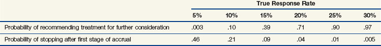
This new design has some nice properties. The maximum number of patients required is the same as before, and, as shown in Table 12-2, the new design still satisfies each of the desired criteria 1 to 3 listed previously. However, if the new treatment has a true response rate of 5% or less, the study has a 0.46 chance of stopping after 15 patients have been accrued, therefore sparing 25 patients from treatment with an inactive regimen.
TABLE 12-2 Operating Characteristics of a Two-Stage Phase II Study Design Allowing Early Stopping for Zero Responses in the First 15 Patients
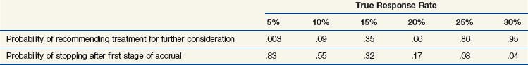
Now consider a design that requires early stopping if only 0 or 1 of the first 15 patients responds; otherwise, 25 more patients are accrued, and the treatment is recommended for further consideration if at least 7 patients respond. This design provides much better protection against the possibility of accruing an excessive number of patients to an ineffective regimen. However, if this design is used, it would be slightly less likely that a truly effective regimen would be recommended for further consideration. Table 12-3 shows the properties of this design.
TABLE 12-3 Operating Characteristics of a Two-Stage Phase II Study Design Allowing Early Stopping for Zero Responses or One Response in the First 15 Patients
Numerous authors discussed optimal strategies for choosing phase II designs, including Gehan,5 Herson,6 Lee, Staquet and Simon,7 Fleming,8 Chang and associates,9 Simon,10 Therneau, Wieand and Chang,11 Bryant and Day,12 and Thall, Simon and Estey.13
Newer Phase II Designs: Randomized Phase II Design
Single-arm phase II designs can demonstrate biologic activity of an agent with relatively small sample size and short study duration. However, the potential for patient selection bias, the evolving methodologies for the assessment of “success” (i.e., changes in CT scanners, changes in response criteria), and a general lack of robustness of historical rates of this type of design result in a high possibility that a positive single-arm phase II trial will be followed by a negative phase III study.14 A potential solution to this fundamental limitation of single-arm phase II designs is the use of a randomized design. For example, two types of randomized phase II designs, the randomized selection designs and the randomized screening designs, have been proposed and used widely.
In a selection design, all arms are considered experimental arms. These could be different new regimens or different doses or schedules of the same regimen. The sample size is calculated to guarantee that with a very small probability, perhaps 10%, an inferior arm (for instance, one in which the response rate is 15% lower) will be selected for the future phase III study. In a standard selection design, the arm with the highest estimated success rate for the primary end point will be recommended for a follow-up phase III study, no matter how small the difference of estimates might be among arms.15 On the other hand, a flexible selection design, or “pick-the-winner” design, will recommend the arm with the best estimated primary end point if the difference is larger than a prespecified criterion.16 Otherwise, toxicities, expense, and other factors will be taken into consideration when making the decision.
If a standard of care is included in the comparison, a screening design should be applied.17 A screening phase II design is similar to a randomized phase III trial but has larger type I and type II errors. For instance, a range of 10% to 20% for both error rates is acceptable. A screening phase II design provides a head-to-head comparison between the experimental regimen and the standard of care using a relatively smaller sample size and clear guidance as to the likelihood of success if the agent is moved forward into phase III testing.
Phase III Trials
It is generally recognized that judging the value of a new therapy by comparing it with historical data may give an erroneous impression of the therapy’s efficacy. Pocock18 related a number of illuminating examples of this phenomenon. Therefore the phase III trial, in which a new agent or modality is tested against an accepted standard treatment in a randomized comparison, is considered the most satisfactory method of establishing the value of the proposed treatment.
Under most circumstances, the goal of a phase III trial is to determine whether the proposed treatment is superior to the standard treatment (superiority trial). Occasionally, the goal is to “show that the difference between the new and active control treatment is small, small enough to the known effectiveness of the active control to support the conclusion that the new test drug is also effective” (noninferiority trial).19 Because the goal of a phase III trial is to make a definitive conclusion regarding a new treatment’s efficacy, enough patients need to be accrued to guarantee a small probability of false-positive results (i.e., declaring that a regimen is effective when in fact it is not) and a large probability of true-positive results (i.e., declaring that a regimen is effective when in fact it is). The probability of false-positive results is also called the size of the study, which usually is limited to 5% or less. The probability of true-positive results is also called the power of the study, which usually is set at 80% to 95%. The primary end points for comparison are usually survival and PFS/DFS, and a common secondary end point is quality of life (QOL). In this section, we discuss the rationale for requiring randomized treatment assignment and stratification in a phase III trial. We introduce the intent to treat principle, and we emphasize the importance of monitoring in ongoing trials.
Stratification of Treatment Assignments
In some cases, it is difficult or even impossible to achieve completely balanced treatment assignments within every combination of the levels of all potential stratification variables. For example, in multicenter cancer clinical trials, it is generally thought to be good practice to balance treatment assignments within each accruing institution because patient selection may differ from institution to institution. However, it is not unusual for cooperative groups in oncology to conduct phase III clinical trials using several hundred accrual sites. Clearly, it would be difficult to stratify completely in the accruing institutions together with other potentially prognostic variables, because the number of resulting combinations of levels of all the stratification variables would be excessive. To circumvent this problem, cooperative groups commonly use algorithms that dynamically maintain nearly balanced assignment of treatments across the levels of all stratification variables marginally but that do not guarantee balance within all combinations of the levels of all of the stratification variables. This approach also results in nearly balanced treatment assignments at all times; this will be beneficial if, as often happens, the characteristics of patients for whom the trial is considered most appropriate in the judgment of accruing physicians tend to change as the trial matures. Details of several such dynamic balancing algorithms may be found in articles by Taves,20 Pocock and Simon,21 Freedman and White,22 and Begg and Iglewicz.23
Intent to Treat
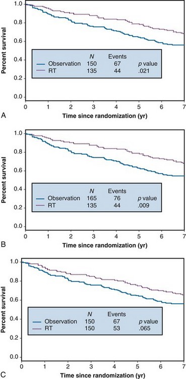
Example 1. A clinical trial was designed to compare the effect of radiation therapy relative to observation in patients with rectal cancer. Three hundred patients were randomized between radiation therapy (arm A) and observation (arm B), 150 to each arm. Suppose that all patients actually received all of their intended therapy and that after 7 years of follow-up, survival curves were as shown in Figure 12-1A. Although the survival curve for patients receiving radiation therapy lies above that for patients in the observation-only arm, suggestive of a benefit from radiation therapy, the difference is not quite statistically significant (p = .058).
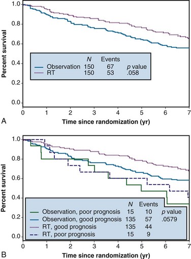
In any clinical trial, the patients who are accrued exhibit considerable variation in their prognoses. Suppose that we could make use of certain prognostic patient characteristics that were unavailable in the analysis summarized previously. Suppose further that by using this new information, we could identify the 10% of patients with the worst prognoses. Then we might redraw the survival curves after stratifying according to risk, resulting in the plots shown in Figure 12-1B. An analysis of these data that takes this stratification into account again yields a p value of .058, which agrees with the p value from the unstratified analysis to three decimal places. This insensitivity of analysis to stratification is a direct consequence of the randomization used in the design of the trial, which tends to balance the poor-prognosis patients equally across the two arms of the trial.
We now consider the possible consequences associated with these three possibilities. Under the assumption that patients’ reasons for refusal of treatment are completely unassociated with prognosis, methods 1 and 2 just presented should lead to estimated treatment differences that are essentially identical to the analysis of Figure 12-1A. If there is a treatment difference, the intent to treat analysis will tend to underestimate this difference because some of the patients who were not irradiated are counted as having received that therapy. The differences in the three analyses should be rather small under this assumption of no association between refusal of treatment and prognosis.
Alternatively, it is rather likely that reasons for refusal of treatment will be associated with patient prognosis. For example, patients with poorer performance status, or their physicians, may be less liable to accept assignment to a treatment that is known to be associated with significant toxicity. Deteriorating health may lead to difficulties in traveling to receive treatment; advancing disease may correlate with a patient’s level of depression or anxiety, which, in turn, may correlate with compliance. Suppose that it is the 10% of patients with the worst prognosis who refuse to accept their radiotherapy. Under these conditions, analysis of the data after deleting the noncompliant patients overstates the effect of radiotherapy, as shown in Figure 12-2A. This is because the worst-prognosis patients are deleted from consideration in arm A, but no similar deletion of poor-prognosis patients is made in arm B. The result is a spuriously significant p value of .021. Treating the noncompliers as though they had been randomized to observation (see Fig. 12-2B) results in an even more serious overstatement of the radiotherapy effect, associated with a p value of less than .009. In contrast, the intent to treat analysis yields a slightly attenuated treatment effect (p = .065) (Fig. 12-2C) but no serious misrepresentation of the true effect.
To summarize, we recommend always performing an intent to treat analysis using all patients as randomized and reporting the results of that analysis in any publication. Further analyses may be performed, especially for noninferiority trials, but one should be aware of potential biases similar to those described previously. Further discussion of these issues can be found in articles by Pocock18 and Gail.24
The data used in Example 1 were generated using the following assumptions. The expected 5-year survival rate for an untreated good-risk patient was .73, and for an untreated bad-risk patient, .54. The reduction in the death rate associated with radiation treatment was assumed to be 20% in each group. For Figure 12-2, we assumed that all the poor-risk patients had an expected 5-year survival rate of .54 because none received treatment.
Monitoring Ongoing Trials
There are different approaches in setting interim monitoring boundaries for superiority. For instance, Pocock25 proposed to spend the type I error (false-positive rate) equally throughout all interim and final analyses. O’Brien and Fleming26 proposed to reserve most of the type I error for the final analysis. The general approach is to set the interim boundaries conservatively so that the trial will not stop early for efficacy unless very convincing evidence is present.
Typically, setting the interim boundaries for futility is not done as conservatively as is setting them for superiority. A nice rule of thumb proposed by Wieand and coauthors27 is as follows: Assuming that a study has a time-to-event primary end point, an interim futility check will be conducted when 50% of events targeted for final analysis have been observed. If the hazard ratio of the experimental treatment versus the control is larger than 1 (i.e., the outcomes on the experimental arm are poorer than those on the control arm at that time), the trial should be stopped for reasons of futility. The rule is simple to follow, and the probability of falsely determining that an experimental regimen is no better than the control situation when, in fact, the experimental regimen actually works is 2% or less.
Survival Analysis
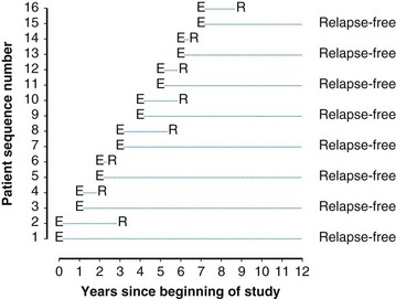
Example 2. Suppose a radiation oncologist decides to review the outcomes of rectal cancer patients treated with radiation therapy. Of primary interest is the determination of the proportion of patients who remain relapse free for 5 years. Suppose patients have been accrued over the past  years, and by chance the patients have started treatment in pairs at intervals of 1 year. Suppose, furthermore, that if no more patients were accrued and the oncologist could wait 5 more years to obtain 5-year follow-up for every patient, he or she would find that half of them were relapse free for more than 5 years. This (unobserved) relapse pattern is shown in Figure 12-3.
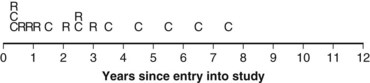
Twelve years after the first patient was entered, the 5-year relapse-free pattern would be as shown in Figure 12-4 (time 0 is the date of entry for each patient). If the investigator had waited 12 years (i.e., until 5-year data for all 16 patients were complete), he or she would have observed that half of the patients were relapse free 5 years after entry (i.e., the 5-year relapse-free rate is .50). Suppose, in fact, that the investigator decided to look at the patients’ experience  years after the first patient had entered. Then the investigator would have observed everything to the left of the vertical line in Figure 12-5. Translated into time from entry, this would be represented as shown in Figure 12-6. In that case, the investigator would have complete 5-year data for seven of the eight patients who relapsed and for three patients who were relapse free at 5 years (those who were entered at year 0, 1, or 2). For the other six patients, his or her knowledge would be that they were relapse free for some length of time less than 5 years. The investigator’s first instinct might be to exclude these six patients from analysis because he or she does not know what their relapse status will be after 5 years of follow-up. Of the remaining 10 patients, 7 are known to have relapsed and 3 are known to be disease free for more than 5 years, so that the estimated relapse-free rate at 5 years is .30. This estimate does not seem to reflect the data accurately.
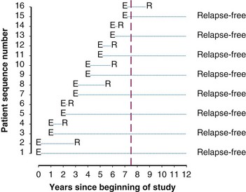
Figure 12-5 Status of follow-up 7.5 years after the first patient was entered in the trial. E, entry; R, relapse.
 years (i.e., did not have a known status at 5 years) and, hence, was excluded. However, the eighth patient (who was entered on the same day) had relapsed by the time of analysis and, therefore, was included. The bias is that patients who relapse have a better chance of being included in the analysis than those who do not relapse. One way to avoid a biased estimate would be to exclude all patients who did not have the potential to be monitored for 5 years. Therefore the oncologist would only be able to use the information from the first six patients entered. In this artificial example, this would have led to a correct estimate of the 5-year relapse-free rate because three of the first six patients relapsed within 5 years.
Kaplan-Meier Method
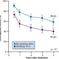
A common way to summarize survival data is to estimate the “survival curve,” which shows—for each value of time—the proportion of subjects who survive at least that length of time. Figure 12-7 shows survival curves for patients with operable breast cancer who have been treated with either preoperative or postoperative chemotherapy (doxorubicin and cyclophosphamide) in a large clinical trial. In this section, we discuss the estimation of survival curves using a method proposed by Kaplan and Meier.28
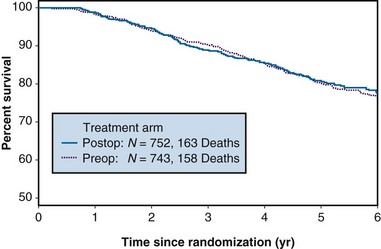
Figure 12-7 Survival of patients with operable breast cancer treated with doxorubicin and cyclophosphamide.
Several excellent references are available that show exactly how a Kaplan-Meier estimate is computed and describe other properties such as the variance of the estimator. A nice summary with formulas for computations can be found in Chapter 2 of Parmar and Machin’s text.29 Here, we offer two examples that provide some insight regarding the Kaplan-Meier method. The first example concerns a data set having no censored observations; the second example extends these ideas to accommodate censored observations.
 , which matches the empirical survival estimate. In fact, the Kaplan-Meier estimate and the empirical estimate always match when they are applied to uncensored data.
The reader may verify that application of the Kaplan-Meier approach to the data in Figure 12-6 will result in an estimate of .45 for the probability of remaining relapse free through 5 years.
Log-Rank Statistic
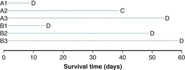
The log-rank statistic deals with the problem of censoring by comparing the groups only when a patient within any of the groups experiences an “event” (if survival times are to be compared across groups, an event would be a death; if times to relapse are to be compared, an event would be a relapse, and so on). This idea is most easily explained in the context of a simple example. Suppose we monitored three patients receiving a standard treatment regimen (this might even be no treatment), which we refer to as treatment A, and three other patients receiving an experimental regimen, which we refer to as treatment B. Suppose, furthermore, that the survival times for the patients receiving treatment A are 10, 40+, and 55 days, respectively, and for the patients receiving treatment B, 15, 50, and 60 days, respectively (a plus sign after a value refers to a censored time (i.e., a patient with a time of 40+ days was last known to be alive at 40 days and no further follow-up is available). These data are represented graphically in Figure 12-8; the three patients receiving treatment A are labeled A1, A2, and A3, and those receiving treatment B are labeled B1, B2, and B3. Deaths are denoted by the letter D, and censored survival times are labeled with the letter C.
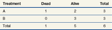
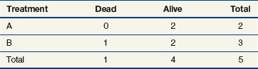
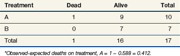
When evaluating the log-rank statistic, the first computation occurs at time t = 10, the time at which the first death is observed. Just before this point in time, all six patients are known to be alive (and, hence, are “at risk” to die at time t = 10). Three of these patients received treatment A and three received treatment B. Exactly one of these six patients is known to have died at time t = 10, and he or she received treatment A. Table 12-4 summarizes the status of patients at this time point. Notice that at the time of this computation there are three patients on each arm. Therefore, if treatment B was equivalent to treatment A and only one death occurred on one arm or the other, there would be a one-half chance that the death is on arm A. In fact, the death is on arm A; hence, we observe one death when the probability of observing a death on arm A is one half (i.e., there is one half more death on arm A than is expected).
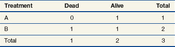
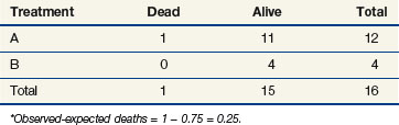
Observations at time t = 15 are listed in Table 12-5. At this point there would be a two-fifths probability that the death would occur on treatment A (if the treatments were equivalent), but the death did not occur on treatment A, so there were two-fifths fewer deaths on arm A than expected (i.e., the observed deaths minus the expected number is  ).
).
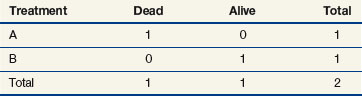
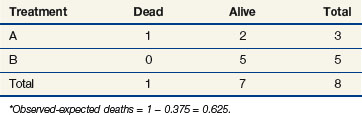
The next computation occurs at time t = 50; observations are listed in Table 12-6. Notice that patient A2 is not included in this table, even though she is not known to have died at any time before t = 50. Because she was lost to follow-up (censored) at time 40, she is no longer “at risk” at time 50. At this time, there would be a one-third probability that the death would occur on treatment A (if the treatments were equivalent), but the death does not occur on treatment A, so there are one-third fewer deaths on arm A than expected (i.e., the observed deaths minus the expected number is  ).
).
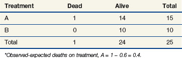
One may go through the same computations at time t = 55 (Table 12-7) and will determine that the number of deaths minus expected deaths on treatment A is  . At time t = 60, all remaining patients are on the same arm, so the observed minus the expected number of deaths must be 0. Adding up the observed minus the expected number of deaths at times 10, 15, 50, and 55, one obtains 2 observed deaths minus 1.733 expected deaths, so that there were 0.27 deaths more than expected on arm A, indicating that this treatment might be harmful. However, one’s intuition is that this is not a significant difference (i.e., such a small difference could easily be attributed to the play of chance), and in fact this is true. Therefore there is no strong evidence in this example that treatments A and B differ.
Stratified Log-Rank Statistic
| 1 to 3 nodes | |
|---|---|
| Treatment A | 91, 160+, 230+ |
| Treatment B | 32, 101, 131+, 155+, 190+, 210+ |
| 4 or more nodes | |
|---|---|
| Treatment A | 11, 22, 42, 63, 72, 110, 120, 141, 155, 180+, 200+, 220+ |
| Treatment B | 51, 83, 110, 170+ |
If we were to ignore our knowledge of the patients’ lymph node status and compute a log-rank statistic as we did before, our computations at times 11 and 91 would be as shown in Tables 12-8 and 12-9. If one completes these computations at each time of death, the total for arm A is 10 observed deaths when 8.85 were expected. This translates to 1.15 excess events on arm A.
The stratified log-rank test provides a method to control for the association of nodal status with patient survival. To illustrate how this occurs, let us recompute the observed and expected deaths at times of 11 and 91 days, but this time we adjust our definition of risk sets to include nodal status. Notice that when we performed these computations for the log-rank test at t = 11 (as shown previously), we estimated the likelihood that the death that occurred was on arm A to be 15/25, based on the fact that 15 of the 25 patients at risk at that time were on arm A. This implicitly assumed that in the absence of a treatment effect, all patients are at the same risk of dying regardless of nodal status. However, the first patient who died was one who had four or more positive nodes. The patients who would be at the same risk of dying as that patient are the other patients with four or more nodes. Because we knew there were 16 patients with four or more nodes who were at risk of dying at t = 11 and that 12 of these patients were on arm A, perhaps we should have estimated the probability to be three quarters that if a patient with four or more nodes died at time t = 11, the patient would be on arm A (given no treatment effect). This is the method used when computing the stratified log-rank test. We now examine the computations at times of 11 and 91 days using this stratified approach (Tables 12-10 and 12-11).
Cox Proportional Hazard Model
The stratified log-rank test as defined previously provides a method to control for the association of nodal status with patient survival. However, in terms of adjusting for additional explanatory variables, the most popular method is the Cox proportional hazard model.30 The Cox model explores the relationship between survival experience and prognostic variables or explanatory variables. It estimates and tests the hazard ratio between different groups. In the Cox regression model, explanatory variables could be continuous (for instance, age or weight or systolic blood pressure), categorical (for instance, gender or race or Eastern Cooperative Oncology Group [ECOG] performance score), or an interaction between different categorical variables. The Cox regression model does not make any parametric assumption about the survival probability distribution of each group; however, it does assume a proportional hazard between two groups. If we use hi(t) and h0(t) to denote the hazards of death at time t for the ith patient and the baseline patient, that is, the patient with all explanatory variables taking values 0, respectively, the proportional hazard model can be expressed as

Current Topics in Phase III Clinical Trials
Surrogate Endpoint
In validating an endpoint as a legitimate surrogate endpoint, a meta-analysis is usually required because relationships presented in one trial may not be generalizable to another. In addition, heterogeneity between the trials included in the meta-analysis strengthens the robustness of results from individual trials. In conducting a meta-analysis, using individual patient data instead of summary data is highly recommended, and, ideally, both positive and negative trials are included. Examples of meta-analyses conducted to examine potential surrogate endpoints can be found in articles by Sargent and colleagues31 and Burzykowski and associates.32
Biomarkers
Validation of a prognostic marker is usually conducted retrospectively in patients treated with placebo or a standard treatment. Validation of a predictive marker could also be conducted retrospectively based on data from a randomized controlled trial.33 However, a prospective randomized controlled trial would be ideal. Two types of clinical designs can be used to validate a predictive marker: a targeted/selection design or an unselected design. A targeted trial enrolls only patients who are most likely to respond to the experimental therapy based on their molecular expression levels. On the one hand, a targeted trial could result in a large savings of patients for other trials. On the other hand, it could miss efficacy in other patients, and miss the opportunity to test the association of the biologic endpoints with clinical outcomes.
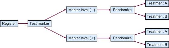
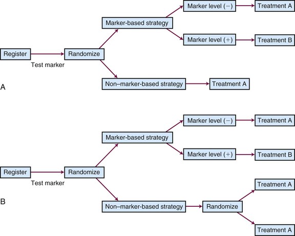
Different types of unselected designs have been proposed and discussed. For instance, the marker-by-treatment interaction design (Fig. 12-9) stratifies patients according to their marker status and randomly assigns patients in each marker group to two different treatments. Hypothesis setting and sample size estimation could be different in each marker-defined subgroup. Either a formal test for marker-by-treatment interaction or a separate superiority test within each marker group could be conducted. Another popular unselected design is the marker-based strategy design (Fig. 12-10), in which the random treatment assignment could be based on the patient’s marker status or could be independent of it. Examples for each type of design can be found in the article by Sargent and colleagues.34
Adaptive Design
An adaptive design could be defined as a design “that allows adaptations to trial procedures (for instance, eligibility criteria, study dose, or treatment procedure, etc.) and/or statistical procedures (for instance, randomization, study design, study hypothesis, sample size, or analysis methods, etc.) of the trial after its initiation without undermining the validity and integrity of the trial.”35 Many types of adaptation could be applied to an ongoing trial. For instance, a study could be resized based on an interim review of the outcomes in the control group. Assume, for example, that in the design of a study, the PFS under the standard of care was assumed to be 12 months. However, on an interim review of accrued data from the control arm, the estimated PFS was 15 months. In this case, more patients need to be accrued for the study or patients need to be followed longer for the same hazard ratio to be detected. No statistical penalty is required for this review, because only data from the control arm have been analyzed.
1 Meinert CL. Clinical Trials: Design, Conduct, and Analysis. Oxford: Oxford University Press; 1989.
2 Goldberg RM, Kaufmann SH, Atherton P, et al. A phase I study of sequential irinotecan and 5-Fluorouracil/leucovorin. Ann Oncol. 2002;13:1674-1680.
3 O’Quigley J, Pepe M, Fisher L. Continual reassessment method. A practical design for phase I clinical trials in cancer. Biometrics. 1990;46:33-48.
4 Wu W, Sargent D. Choice of endpoints in cancer clinical trials. In: Kelly K, Halabi S, editors. Fundamentals of Oncology Clinical Trials: The Art and Science Behind Successful Clinical Trials. New York: Demos Medical, 2008.
5 Gehan A. The determination of the number of patients required in a follow-up trial of new chemotherapeutic agent. J Chronic Dis. 1961;13:346-353.
6 Herson J. Predictive probability early termination plans for phase II clinical trials. Biometrics. 1979;35:775-783.
7 Lee YJ, Staquet M, Simon R. Two-stage plans for patient accrual in phase II cancer clinical trials. Cancer Treat Rep. 1979;63:1721-1726.
8 Fleming TR. One-sample multiple testing procedure for phase II clinical trials. Biometrics. 1982;38:143-152.
9 Chang MN, Therneau TM, Wieand HS, Cha S. Designs for group sequential phase II clinical trials. Biometrics. 1987;43:865-874.
10 Simon R. Optimal two-stage designs for phase II clinical trials. Control Clin Trials. 1989;10:1-10.
11 Therneau TM, Wieand HS, Chang M. Optimal designs for a grouped sequential binomial trial. Biometrics. 1990;46:771-781.
12 Bryant J, Day R. Incorporating toxicity considerations into the design of two-stage phase II clinical trials. Biometrics. 1995;51:1372-1383.
13 Thall PF, Simon RM, Estey EH. Bayesian sequential monitoring designs for single-arm clinical trials with multiple outcomes. Stat Med. 1995;14:357-379.
14 Tang H, Foster NR, Grothey A, et al. Comparison of error rates in single-arm versus randomized phase II cancer clinical trials. J Clin Oncol. 2010;28(11):1936-1941.
15 Simon R, Wittes RE, Ellenberg SS. Randomized phase II clinical trials. Cancer Treat Rep. 1985;69:1375-1381.
16 Sargent DJ, Goldberg RM. A flexible design for multiple armed screening trials. Stat Med. 2001;20:1051-1060.
17 Rubinstein LV, Korn EL, Freidlin B, et al. Design issues of randomized phase II trials and a proposal for phase II screening trials. J Clin Oncol. 2005;23(28):7199-7206.
18 Pocock SJ. Clinical Trials: A Practical Approach. New York: Wiley; 1984. pp 182-186
19 Guidance for Industry Non-Inferiority Clinical Trials. U.S. Department of Health and Human Services, Food and Drug Administration, March 2010. Available at www.fda.gov
20 Taves DR. Minimization. A new method of assigning patients to treatment and control groups. Clin Pharmacol Ther. 1974;15:443-453.
21 Pocock SJ, Simon R. Sequential treatment assignment with balancing for prognostic factors in the controlled clinical trial. Biometrics. 1975;31:103-115.
22 Freedman LS, White SJ. On the use of Pocock and Simon’s method for balancing treatment numbers over prognostic factors in the controlled clinical trial. Biometrics. 1976;32:691-694.
23 Begg CB, Iglewicz B. A treatment allocation procedure for sequential clinical trials. Biometrics. 1980;36:81-90.
24 Gail MH. Eligibility exclusions, losses to follow-up, removal of randomized patients, and uncounted events in cancer clinical trials. Cancer Treat Rep. 1985;69:1107-1113.
25 Pocock SJ. Group sequential methods in the design and analysis of clinical trials. Biometrika. 1977;64(2):191-199.
26 O’Brien PC, Fleming TR. A multiple testing procedure for clinical trials. Biometrics. 1979;35(3):549-556.
27 Wieand S, Schroeder G, O’Fallon JR. Stopping when the experimental regimen does not appear to help. Stat Med. 1994;13:1453-1458.
28 Kaplan EL, Meier P. Nonparametric estimation from incomplete observations. J Am Statist Assoc. 1958;53:457-481.
29 Parmar KB, Machin D. Survival Analysis: A Practical Approach. New York: Wiley; 1995.
30 Cox DR. Regression models and life-tables (with discussion). J Roy Statist Soc Ser B. 1972;34:187-220.
31 Sargent DJ, Wieand HS, Haller DG, et al. Disease free survival versus overall survival as a primary end point for adjuvant colon cancer studies. Individual patient data from 20898 patients on 18 randomized trials. J Clin Oncol. 2005;23(34):8664-8670.
32 Burzykowski T, Buyse M, Piccart-Gebhart MJ. Evaluation of tumor response, disease control, progression-free survival, and time to progression as potential surrogate end points in metastatic breast cancer. J Clin Oncol. 2008;26(12):1987-1992.
33 Simon RM, Paik S, Hayes DF. Use of archived specimens in evaluation of prognostic and predictive biomarkers. J Natl Cancer Inst. 2009;101(21):1446-1452.
34 Sargent DJ, Conley BA, Allegra C, Collette L. Clinical trial designs for predictive marker validation in cancer treatment trials. J Clin Oncol. 2005;23(9):2020-2027.
35 Chow SC, Chang M. Adaptive design methods in clinical trials—A review. Orphanet J Rare Dis. 2008;3:11.