[level-membership-for-anesthesiology-category]
Quantitative Doppler
Christopher J. Gallagher, Christina Matadial and Jadelis Giquel
Types of Velocity Measurements
Here I think they’re driving at pulsed-wave Doppler versus continuous-wave Doppler. (It’s tough going through this and wondering “What are they thinking?”) To review, then, pulsed-wave Doppler takes a specific look at a specific velocity at a specific place. The pulse wave (PW) transducer is used as both a receiver and transmitter of ultrasound waves. A complete cycle of transmission waiting and receiving is called the pulse repetition frequency (PRF). The greater the depth of interrogation of the pulsed ultrasound beam the longer the waiting period. Therefore, the deeper the interrogation, the lower the PRF, and the lower the maximal velocity that can be measured. Pulsed-wave ultrasound is used to provide data for Doppler sonograms and color flow images.
High-Frame Rate-Doppler
Another thing they might be driving at here is PISA, the proximal iso velocity surface area.
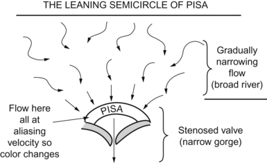
This, too, is gone over ad nauseum in Chapter 3, but here goes. As blood flow converges toward a tight spot (Analogy? Think of a broad river coming to a narrow gorge), the flow will speed up. At a certain concentric area, the flow should all be at the same speed as the “chaos” of a broad river becomes the “organized tightness” of a narrow channel. This area will, when measured by color flow Doppler, hit the Nyquist limit and will start aliasing. Red flow will become blue, for example, in a semicircle. You can measure the area of this by the equation

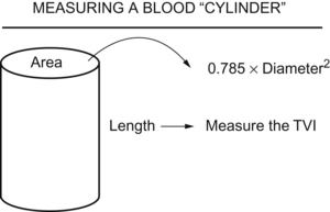
Volumetric Measurements and Calculations
This gets into the realm of the material in Chapter 3, the volume equations you use to measure valve areas, cardiac outputs, stroke volumes, and the like. The sample problems in that chapter illustrate better than this explanation, but here goes.
Valve Gradients, Areas, and Other Measurements
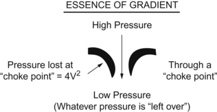
The gradient, or change in pressure, across a valve is measured by the Bernoulli equation:

Example 1: The velocity across a stenotic mitral valve is 4 meters/second. What is the gradient?


The unknown in this equation is the area of the aortic valve.

Cardiac Chamber and Great Vessel Pressures
Figuring this stuff (again, see examples in Chapter 3) requires the Bernoulli equation and one commonsense principle. In the problem you’ll wrestle with, you’ll be given a valve with a velocity across the valve. Use the Bernoulli equation to figure what the pressure gradient is across that valve. So far so good.

If you have, say, mitral stenosis, then during diastole, the high-pressure area will be the left atrium, the pressure gradient will be “pressure lost” crossing the mitral valve as blood struggles to get into the left ventricle, and the “leftover” pressure will be the left ventricular pressure. (Assuming no aortic regurgitation muddies the waters.)


then you can figure any of these “what’s the pressure in chamber or vessel X?” questions.
Tissue Doppler
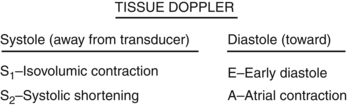
During the meeting they showed some tissue Doppler, but not too much. Just know that it exists and know what S1, S2, E velocity, and A velocity are.
Questions
1. What is the major advantage of pulse wave Doppler?
2. Pulse wave Doppler is best to determine which of the following:
3. CWD is best to determine which of the following:
4. In calculating cardiac output using Doppler method, the LVOT area × LVOT flow velocity equals:
5. Which of the parameters (measured incorrectly) will most likely affect calculation of the cardiac output:
Answers
1. B. The major advantage of pulse wave Doppler is the ability to determine the Doppler shift at a precise location. This ability is called range resolution or range discrimination.
3. B. The major advantage of continuous wave Doppler is the ability to accurately measure high velocities of blood flow. The major disadvantage is range ambiguity.
[/level-membership-for-anesthesiology-category][not-level-membership-for-anesthesiology-category]
Quantitative Doppler
Christopher J. Gallagher, Christina Matadial and Jadelis Giquel
Types of Velocity Measurements
Here I think they’re driving at pulsed-wave Doppler versus continuous-wave Doppler. (It’s tough going through this and wondering “What are they thinking?”) To review, then, pulsed-wave Doppler takes a specific look at a specific velocity at a specific place. The pulse wave (PW) transducer is used as both a receiver and transmitter of ultrasound waves. A complete cycle of transmission waiting and receiving is called the pulse repetition frequency (PRF). The greater the depth of interrogation of the pulsed ultrasound beam the longer the waiting period. Therefore, the deeper the interrogation, the lower the PRF, and the lower the maximal velocity that can be measured. Pulsed-wave ultrasound is used to provide data for Doppler sonograms and color flow images.
High-Frame Rate-Doppler
Another thing they might be driving at here is PISA, the proximal iso velocity surface area.
This, too, is gone over ad nauseum in Chapter 3, but here goes. As blood flow converges toward a tight spot (Analogy? Think of a broad river coming to a narrow gorge), the flow will speed up. At a certain concentric area, the flow should all be at the same speed as the “chaos” of a broad river becomes the “organized tightness” of a narrow channel. This area will, when measured by color flow Doppler, hit the Nyquist limit and will start aliasing. Red flow will become blue, for example, in a semicircle. You can measure the area of this by the equation
Volumetric Measurements and Calculations
This gets into the realm of the material in Chapter 3, the volume equations you use to measure valve areas, cardiac outputs, stroke volumes, and the like. The sample problems in that chapter illustrate better than this explanation, but here goes.
Valve Gradients, Areas, and Other Measurements
The gradient, or change in pressure, across a valve is measured by the Bernoulli equation:
Example 1: The velocity across a stenotic mitral valve is 4 meters/second. What is the gradient?
[/not-level-membership-for-anesthesiology-category]
