Introduction to ultrasound

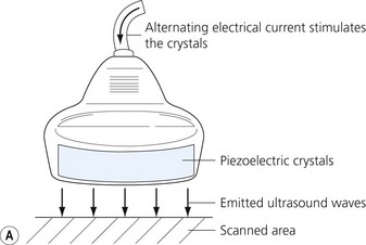
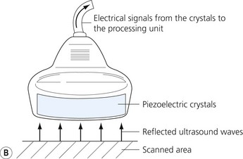
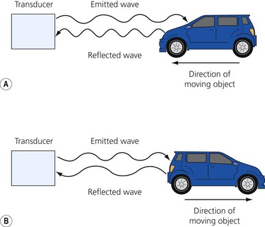
Ultrasound is a mechanical wave with frequencies over 20 000 Hz. Ultrasound used in medicine is generated and sensed by piezoelectric crystals. The ultrasound transducer incorporates a battery of piezoelectric crystals. When scanning, the transducer switches quickly between transmitter and receiver modes. When in transmitting mode, the piezoelectric crystals are stimulated by electrical energy, vibrate and emit ultrasound waves. In the receiver mode the crystals are hit by the ultrasound waves reflected from the tissues (Fig 7.1). The resultant mechanical stimulation of the crystals is converted to electrical signals, which are processed and ultimately create the image we see on the screen.

Figure 7.1 (A) Stimulated by alternating electric current, the piezoelectric crystals vibrate and emit ultrasound waves. (B) The reflected waves hit back the crystals, which undergo conformational changes and generate electric current.

Why understanding ultrasound physics and how to use an ultrasound machine is important

Here are some examples:

Why don’t I see my needle?

When a sound wave hits a reflective surface, the resultant reflection is at an angle corresponding to the incidence angle. When the ultrasound beam hits a needle at an inappropriate angle, the reflected wave will not reach the transducer and there will be no image of the needle (Fig 7.2).

Why cannot I see the deeper structures?

Tissues absorb ultrasound waves. The higher the frequency, the higher the absorption. Thus high frequency transducers are less suitable for visualization of deeper structures (Fig 7.3).

Why is the artery blue?

The color Doppler allows us to visualize moving particles. When the particles move towards the ultrasound transducer by convention they are visualized in red, when they move away from the ultrasound transducer, in blue. Thus, if we orient the ultrasound transducer against the flow, we get red image of the respective vessel. The same vessel will visualize blue if we turn the ultrasound transducer in the direction of the flow (Fig 7.4).

Figure 7.2 (A) Impact angle 90°: the reflected beam reaches the transducer and generates good image. (B) Impact angle 80°: there is partial loss of signal and the image is degraded. (C) Impact angle 30°: the reflected signal does not reach the transducer and the image is lost.

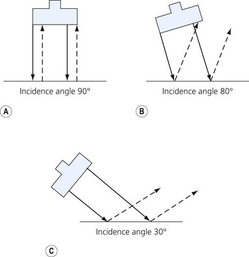
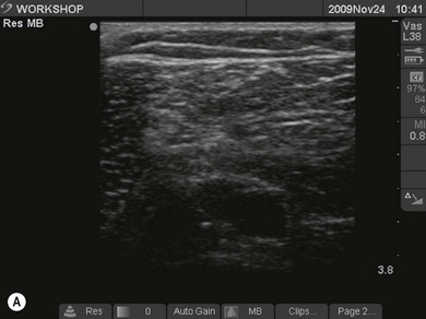
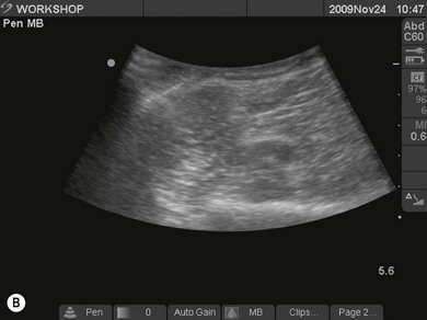
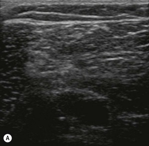
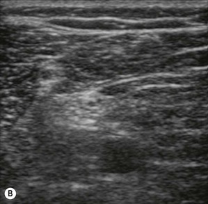
Figure 7.3 (A). High frequency transducer: deep structures do not visualize due to the absorbtion of the ultrasound. Note the good resolution at superficial level. (B) Low frequency transducer: deep structures visualized due to the better penetration of the ultrasound. Note the image has lower resolution, compared with Fig. 7.3A.

Figure 7.4 (A) Transducer tilted against the direction of the flow: the artery is visualized in red. (B) Transducer tilted in the direction of the flow: the artery is visualized in blue. (C) Transducer perpendicular to the flow: there is no Doppler shift and the artery is visualized in black.

Ultrasound physics

Figure 7.5 (A) When the object is moving towards the transducer, the reflected waves have increased frequency. (B) When the object is moving away from the transducer, the reflected waves have lower frequency.

Figure 7.6 (A) Insufficient gain. Note the deep structures are not visualized well. (B) Optimal gain. Note the overall good resolution and the improved visualization of the deeper structures. (C) Excessive gain. Note the blurred image resulting in poor resolution.

Table 7.1 The acoustic impedances of selected body tissues

Figure 7.7 Scan of the axilla. L: fat tissue; B: bone; M: muscle; F: fascia; V: vessel; N: nerve.

The ultrasound machine

The ultrasound machine consists of a transducer (acting as transmitter and receiver), main unit (generating pulses for the transmitter, processing the impulses from the receiver, control unit, memory) and a display.

The transducer

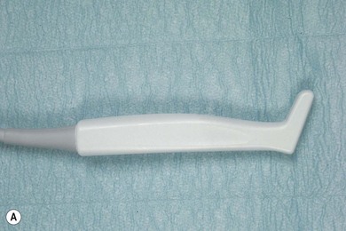
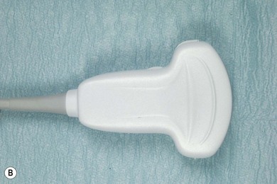
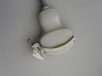
Transducers vary in size, shape, frequency range and number of piezoelectric crystals. For superficial blocks, a high frequency transducer (7–15 MHz) will provide better axial resolution (i.e. better ability to distinguish as separate structures dots lying along the path of the ultrasound beam) (Fig. 7.3). The more piezoelectric crystal elements, the better the resolution. A lower frequency transducer (1–5 MHz) is more appropriate for deeper blocks as there is less absorption and thus better signal from the deeper structures (Fig. 7.3). Transducers with a small footprint (i.e. hockey stick transducers) are useful in children or where space is limiting (Fig. 7.8). Wider (with large footprint) and curvilinear transducers (sector) allow for visualization of a bigger area and thus may be helpful in visualizing landmark structures at the same time as the nerves of interest (Fig. 7.8).

Figure 7.8 (A) A hockey stick transducer. (B) A curvilinear transducer.

The control unit

The control unit allows for adjusting the depth of the image, the gain, focus, to select different visualization modes etc. (Fig. 7.9).

Figure 7.9 The control unit. Note the controls for setting depth, gain, imaging mode etc.

Selecting the appropriate depth is the first step when scanning. The target structure should be in the center of the imaging field where the best resolution is possible. Depth should also accommodate other important anatomical relations.

By manipulating the gain one can improve the image quality. This may involve increasing as well as decreasing the gain (Fig. 7.6).

The focus refers to the depth at which best lateral resolution is achieved (lateral resolution refers to the ability to visualize two dots lying side by side as separate). The transducers come with preset or adjustable focus depth. In either case, the operator should try to match the focus depth with the depth of the object of interest.

Ultrasound machines come with a selection of scanning modes optimized for different applications (nerve block mode, vascular mode, echocardiography mode etc.).

Spatial compound imaging is based on combining images taken at different beam angles into one final image. This technique allows for better visualization of the scanned area.

Beam steering allows for adjustment of the angle of the ultrasound beam leaving the transducer. This is helpful in needle visualization.

Ultrasound tissue appearance

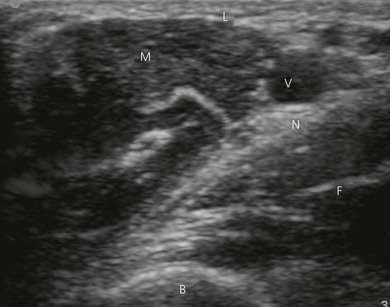
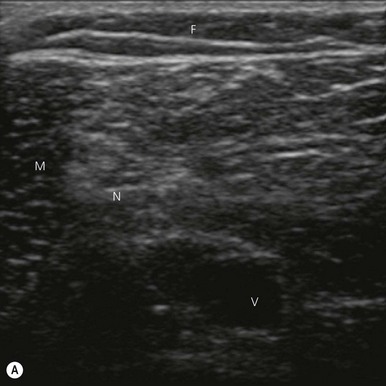
Fat tissue is usually located most superficially (appears on top of the screen), is hypoechoic with interspersed irregular brighter lines of connective tissue (Fig 7.7).

Muscle is hypoechoic (though appears brighter than the fat tissue), with more granular texture, and is surrounded by a hyperechoic fascial sheath (Fig 7.7).

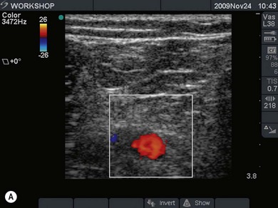
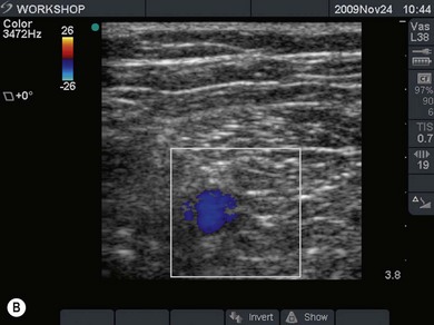
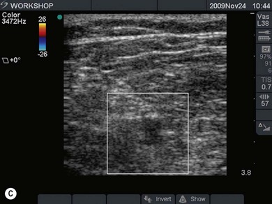
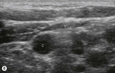
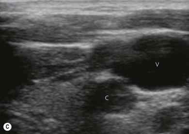
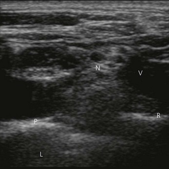
Vessels are anechoic (Fig. 7.10), compressible (veins more than arteries) (Fig 7.10), and pulsatile (usually only the arteries). Doppler will visualize flow (usually continuous for veins and pulsatile for arteries) (Fig 7.4). One can distend a collapsed vein (for example when scanning in the cervical area) by asking the patient to perform a Valsalva maneuver (Fig 7.10).

Figure 7.10 (A) Scan of the interscalene area. M: muscle; V: internal jugular vein; C: carotid artery; R: nerve roots of the brachial plexus. Note the nerve roots visualize as hypoechoic vessel-like structures. (B) Pressure applied to the transducer. Note the vein (V) is compressed. C: carotid artery. (C) The patient is performing Valsalva maneuver. Note the distended vein (V). C: carotid artery.

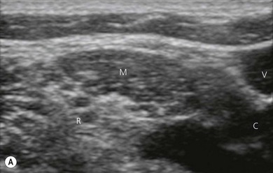
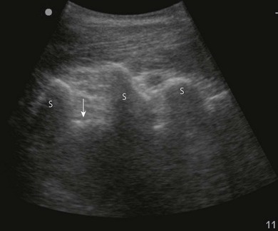
Bone is highly reflective. It visualizes as a hyperechoic band, behind which there is an acoustic shadow due to poor penetration (Fig 7.7).

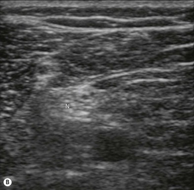
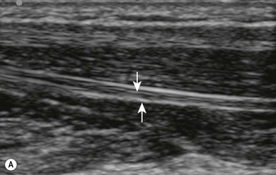
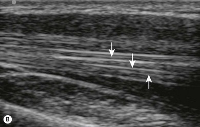
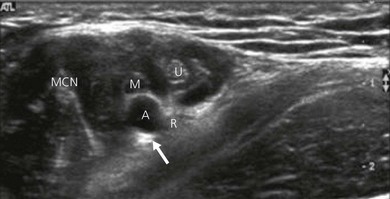
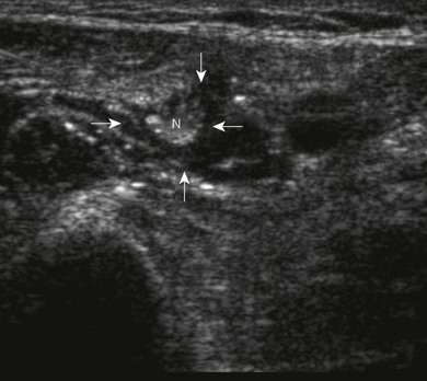
Nerve imaging varies with the location. The proximal parts (i.e. nerve roots when scanning the interscalene area) are rich in nerve tissue and appear black or hypoechoic (similar to vessels) (Fig 7.10). As the brachial plexus runs distally (i.e. supraclavicular area), the proportion of connective tissue increases and the nerve has a grape-like appearance (Fig. 7.11). Further distally in the upper limb, the connective tissue dominates and the nerves appear more hyperechoic (Fig 7.7), or may display a honeycomb pattern (Fig. 7.12). The fascicles are hypoechoic dots with a surrounding hyperechoic rim (epineurium). Anisotropy can affect the ultrasound appearance of nerves (Fig. 7.13). The above comments relate to transverse imaging of nerves. On longitudinal imaging, nerves have a fascicular pattern unlike the fibrillar pattern of tendons (Fig. 7.14).

Figure 7.11 Scan of the supraclavicular area. R: rib; P: pleura; L: lung tissue; V: vessel; N: nerve. Note the grape-like appearance of the brachial plexus (hyperechoic epineurium with large hypoechoic zones comprised of nerve tissue) as well as the drop-out of signal below the rib.

Figure 7.12 (A) Scan of the wrist. T: tendon; M: median nerve; U: ulnar nerve; A: ulnar artery. Note the honeycomb appearance of the median nerve. (B) Another scan of the wrist. Note the similarity of the median (M) and ulnar (U) nerves to the nearby tendons (T). A: ulnar artery.

Figure 7.13 (A) Scan of the popliteal area. F: fat tissue; M: muscle; V: vessel; N: nerve. Note the nerve appears very similar to the surrounding muscle tissue. (B) Demonstration of anisotropy. By slightly tilting the transducer, the nerve visualizes much more clearly.

Figure 7.14 (A) Long axis scan of a nerve. Note the fascicular pattern: long fascicles of hypoechoic nerve tissue (arrows) with interspersed irregular hyperechoic lines representing the epineurium. (B) Long axis scan of a tendon. Note the fibrillar pattern: multiple long hyperechoic lines (arrows), representing the connective tissue.

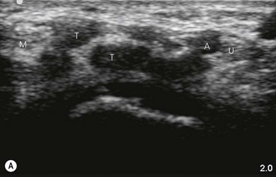
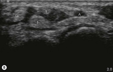
Tendons are hyperechoic and often look similar to peripheral nerves (Fig 7.12). There are some tips that help to differentiate them. When scanning dynamically, one can follow the course of a tendon and observe it merging into a muscle. Nerves are continuous, and can be demonstrated to change course or give divisions when scanned along their course. If we ask the patient to activate the respective muscles, there is more obvious movement of the tendons compared to the nerves near them.

Fascias appear very bright (hyperechoic) (Fig 7.7).

Pleura visualizes as a hyperechoic line, while the lung tissue is hypoechoic (Fig 7.11). Occasionally, one can see a comet-tail sign under the pleura caused by reverberation (see below) at the pleural interface.

Lymph nodes are more likely to be detected in particular anatomic regions (e.g. groin). They have a hypoechoic centre, are non-compressible, color Doppler will not detect flow, and when the ultrasound transducer is moved, they disappear, unlike the vessels, which can be followed longitudinally.

Artifacts

Artifacts can be defined as absence of imaging of an existing anatomical structure, distorted image, or visualization of a non-existent anatomical structure.

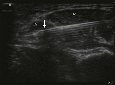
Anisotropy refers to the variable echogenicity of tissues when the incidence angle of the ultrasound beam is changed. By angling the transducer more distally or proximally one can significantly improve the visualization of a scanned nerve (Fig 7.13).

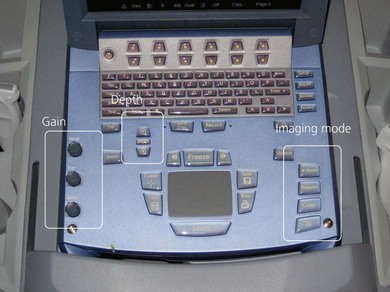
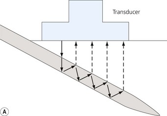
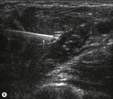
Loss of image. There are many reasons why an anatomical structure is not seen with ultrasound. The following are some examples. When the contact between the transducer and the skin is incomplete (because of insufficient amount of coupling agent with resultant air pockets, or when the one side of the ultrasound transducer is lifted), there will be drop-out areas (Fig. 7.15). Another reason for loss of image is insufficient depth or gain (Fig. 7.6), or usage of a high frequency ultrasound transducer for imaging deep structures (Fig. 7.3). When the impact angle of the ultrasound beam is different from 90°, the reflected waves may not reach the transducer (Fig 7.2). The ultrasound beam is extremely thin. In order to visualize longitudinally another thin structure (i.e. a needle or a nerve), the beam has to be perfectly aligned to it. This skill is difficult to master and requires a lot of practice. Minimal rotation or tilting of the transducer leads to loss of the image (Fig. 7.16).

Figure 7.15 Air pocket (A) between the transducer and the skin, caused by lack of a coupling agent. Note the signal dropout (D) beneath.

Figure 7.16 (A) Transducer and needle not aligned. The needle (N) does not visualize fully. (B) By rotating and/or sliding the transducer, alignment is achieved and the needle tip (arrow) appears on the screen.

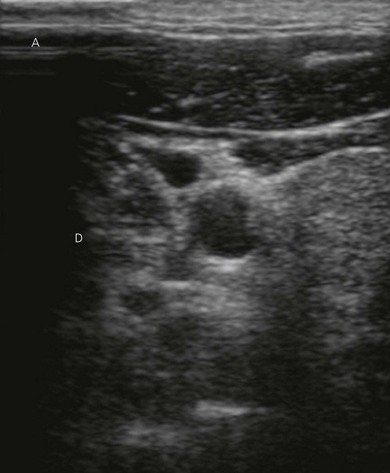
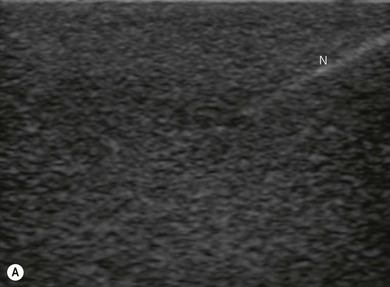
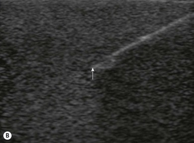
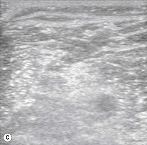
Image resolution poor. Too much gain can cause all the tissues to appear hyperechoic and blur the differences between them (Fig. 7.6). Appropriate manipulation of the gain control will improve the image quality. Using a higher frequency ultrasound transducer may improve image resolution further (Fig. 7.3).

Bayonet artifact. Sometimes a transducer may overlie two adjacent areas that allow ultrasound to travel with different speeds. A needle passing through these two areas may visualize as broken because the ultrasound waves passing through the ‘higher-velocity’ tissue will reach the transducer faster and will give the impression that they come from a more shallow layer than the waves coming from the ‘lower-velocity’ tissues (Fig. 7.17).

Figure 7.17 Bayonet artifact. Note the two adjacent tissue areas conducting ultrasound at different speeds. This results in the needle appearing to be deformed on the screen. A = artery, M = muscle.

Reverberation. Reverberation occurs when repeated reflection occurs between two strongly reflective surfaces (Fig. 7.18). Instead of a single reflected wave there is a series of waves reaching the receiver one after another, giving the false impression of multiple hyperechoic layers in the scanned area (Fig. 7.18). If this occurs, the operator should try to reduce the gain.

Figure 7.18 (A) Reverberation: ultrasound wave repeatedly reflected between two surfaces generates secondary echoes. (B) One needle visualizing as more than one due to reverberation (arrow).

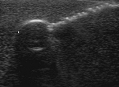
Posterior enhancement occurs when scanning over a fluid filled space (i.e. a cyst). The tissue immediately under this space may appear hyperechoic due to the significant reflection at the tissue interface and the good conductance of the reflected waves through the fluid back towards the transducer (Fig. 7.19). Care needs to be taken interpreting sonoanatomy here.

Figure 7.19 Posterior enhancement artifact (arrow). A: axillary artery; M: median; U: ulnar; R: radial nerves; MCN: musculocutaneous nerves.

Posterior shadowing can be seen as a dropout of signal behind tissues that poorly conduct ultrasound (i.e. bone or air filled spaces like bowels) (Fig. 7.11).

Ergonomics

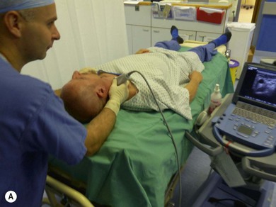
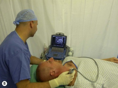
When performing ultrasound-guided nerve blocks, the operator, the needle transducer interface, and the ultrasound screen should be in one line if possible. The angle of the display should be adjusted for optimal visibility (Fig. 7.20). The configuration has to provide maximal comfort and stability for the patient as well as the operator. Both hands of the operator (the scanning and the needling hand) should rest on the patient to ensure stability and thus optimal control (Fig. 7.21). The necessary procedural equipment needs to be within easy reach and an assistant is desirable.

Figure 7.20 (A) Example of good orientation of operator, patient and ultrasound screen. (B) Example of poor orientation. Note the operator has to turn his/her head in order to look at the screen.

Figure 7.21 (A) Correct positioning of operator’s hands. The position shown ensures stability when manipulating the transducer and the needle. (B) This is an example of poor position, as the way the hands hold the transducer and the needle does not provide stability.

Scanning technique and anatomical survey

General considerations

Transverse (short axis, cross-sectional) scanning involves orientating the transducer perpendicular to the long axis of the anatomical structure of interest (Fig. 7.7). When using short axis views, the identification of nerves and the confirmation of the spread of local anesthetic is facilitated (Fig. 7.22). Tilting the ultrasound transducer can dramatically improve the image (Fig. 7.13), while slight tilting or sliding usually does not cause loss of the target (unlike when using longitudinal scanning).

Figure 7.22 The donut sign (arrows) – local anesthetic spreading in a circle around the nerve (N).

Orientating the transducer parallel to the long axis of the anatomical structure of interest gives a longitudinal (long axis) view. This sometimes can be helpful to confirm that a structure is a nerve (Fig 7.14). This scanning orientation is more difficult as the ultrasound transducer and anatomical structure have to be perfectly aligned in order to produce an image of the structure.

Scanning technique

Set up an ergonomic configuration as mentioned above. Select an ultrasound transducer appropriate for the depth of the scanned area. Obey the principles of asepsis. Apply coupling gel. The transducer has to be in sufficient contact with the skin. Avoid excessive pressure, as this may cause image distortion, compress vessels or push structures of interest out of the visualized field. It may also hurt the patient.

The basic movements when manipulating the transducer are sliding, rotation and tilting.

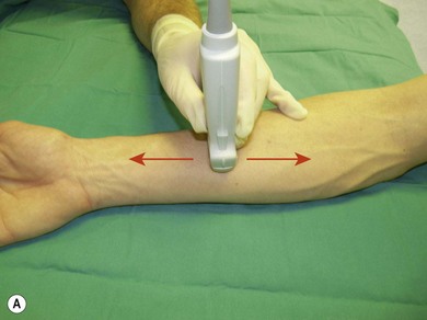
Sliding allows one to position the transducer over the area of interest. It encompasses moving the transducer on the proximal/distal or medial/lateral axis (Fig. 7.23).

Figure 7.23 (A) Sliding. (B) Rotation. (C) Tilting.

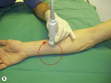
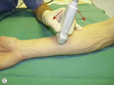
Following this, the depth of imaging should be adjusted, thus enlarging the target while keeping the necessary landmark structures in view. Consider adjusting the gain and focus. Next, one can rotate the transducer to achieve optimal orientation (short or long axis) against the object of interest (Fig 7.23). The latter should be in the centre of the screen. The last step is tilting (Fig 7.23). These maneuvers are important in needle identification.

Practicalities of ultrasound-guided regional anesthesia

Point of entry and depth. Ultrasound helps selection of needle entry and outlines depth required. The point of needle entry should be a distance of 1 cm from the ultrasound transducer. This facilitates asepsis and the free hand technique of needle intervention. Ultrasound can also be used to facilitate blocks without guidance. Here ultrasound is used to identify anatomy and provide valuable information, such as depth of target structures. For example, one can visualize the position of the spinous and transverse processes and measure the depth of the epidural and the paravertebral spaces (Fig. 7.24).

Figure 7.24 Longitudinal midline scan at L3/4 level. Processus spinosus (S), epidural space (arrow). Note the depth of the epidural space can be determined.

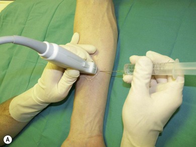
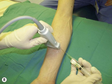
Needle visualization. The key to visualizing needles in long axis is perfect alignment of ultrasound beam and needle. The ultrasound beam is narrow and thus practice cannot be replaced. Never advance the needle without visualization. Adjust the transducer (sliding, tilting, rotation, pressure) rather than the needle, as this is safer and causes less discomfort for the patient. The more parallel the needle is to the ultrasound beam, the easier it is to see. Beam steering and compound imaging may be of help. Large bore needles visualize better. The industry is working on solutions to improve needle shaft and needle tip visibility (e.g. echogenic coating). Mechanical needle guides help to maintain the transducer – needle alignment (Fig. 7.25). A free hand technique rather than the use of needle guides is favored, due to the greater flexibility it allows.

Figure 7.25 Mechanical needle guide.

Local anesthetic spread. Proper placement of local anesthetic is paramount to achieve fast and sufficient nerve block. The solution should encircle the nerve, thus outlining it (the donut sign) (Fig. 7.22). Avoid injecting air bubbles, as these cause acoustic shadowing and deteriorate the image (Fig. 7.26).

Figure 7.26 Acoustic shadow degrading the image after air bubbles were injected (arrow).

Catheter placement. While it is impractical to try to visualize the catheter tip movement as it is advanced, with ultrasound one can demonstrate the spread of local anesthetic close to the nerves of interest.