Chapter 1 Principles of CMR
Basic physics
MRI is based on nuclear magnetic resonance, the phenomenon of the resonance of atomic nuclei in response to radiofrequency (RF) waves.
At equilibrium within a magnetic field, overall proton alignment is in the direction of the main magnetic field and they have net longitudinal magnetization. This equilibrium can be disturbed by transmission of RF energy at the precession frequency of the proton which is 63 megaHertz (MHz) for water protons at 1.5 Tesla (T)—the strength of most commercially used magnets (Figure 1.1).
Localization of anatomical position within a selected imaging slice or volume is done with the application of frequency- and phase-encoding gradients. The corresponding direction of application of these gradients is known as the frequency encode or phase encode direction. With modifications of the phase-encoding gradients flowing blood can be differentiated from stationary anatomy via alterations in the phase of the MR signal. The velocity of material is proportional to the phase change or phase shift caused by its movement during gradient application.
Main sequences
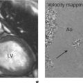
There are two fundamental types of sequence commonly used in CMR: gradient echo (GE) and spin echo (SE). As a general rule, with GE sequences both blood and fat appear white and so this technique is also known as white-blood imaging (Figure 1.2a). By contrast, in SE sequences blood is usually black but fat is white, giving rise to the term black-blood imaging (Figure 1.2b). SE sequences are more useful for anatomical imaging as opposed to the functional imaging performed with GE sequences. Variations of GE sequences are fast low-angle shot (FLASH), fast imaging with steady-state free precession (SSFP), and velocity mapping. GE imaging also forms the basis of the inversion recovery technique.
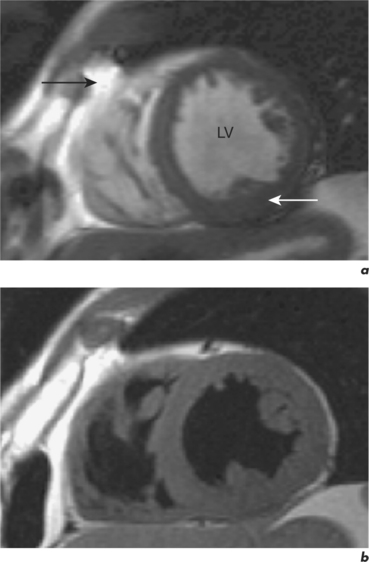
Areas of focal myocardial dysfunction and abnormal flow patterns are readily visualized with the technique of cine imaging using SSFP (or cines). Cines are obtained by rapid repetition of a variant of the basic GE sequence to obtain a series of cardiac images at progressively advancing points of the cardiac cycle which when put together form a cine loop. The weighting of SSFP sequences depends on the ratio of T2/T1, therefore most fluids and fat have a high signal and appear white. However, muscle and many other solid tissues have a long value for T1 and a short value for T2. This means that their signal intensity is reduced to shades of grey (Figure 1.2a). In addition to cines, the SSFP sequence can also be applied as a two-dimensional (2D) single-shot technique, as a real-time technique (not requiring breath holding or electrocardiogram (ECG) triggering), and as a three-dimensional (3D) volume scan.
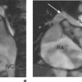
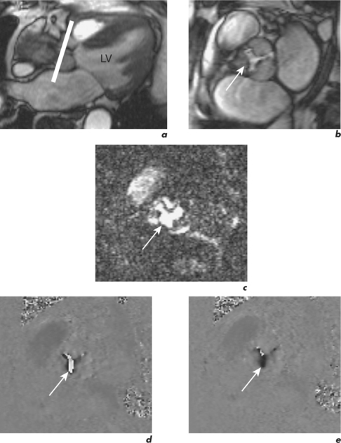
Velocity mapping (or flow velocity mapping) techniques can determine the average velocity within a single imaging voxel, typically 1 ×1 ×10 mm3. The operator selects the required plane and sets a maximal encoding velocity (Venc; Figure 1.3). The initial Venc used is an approximation of the velocity expected based on factors such as clinical history, the type of valve or conduit lesion, and images already acquired. The Venc represents the practical upper limit of velocities that can be depicted unambiguously and should ideally be set to a numerical value just greater than the true velocity. Problems occur if it is set much higher or lower than this value—with the former leading to less sensitivity and the latter causing misrepresentation via the phenomenon of aliasing. Velocity aliasing is when the flow appears to be in the opposite direction and is characterized by a sudden transition of white-toblack or vice versa within the chosen flow region (Figure 1.3d). To eliminate or reduce aliasing a higher Venc must be set and the velocity mapping sequence repeated (Figure 1.3e). The maximal velocity of jets under interrogation should only be determined from the Venc-optimized images. Aliasing is also noted with 2D Doppler echocardiography and the technique of velocity mapping gives similar information. Subjects are asked to suspend their breathing for measurement of peak velocities using this method, which takes approximately 20 seconds to perform. An example of its use is for the quantification of peak velocity in valvular stenosis. Velocity mapping sequences are also used to calculate overall flow in a major vessel through the cardiac cycle and so can be used for quantification of regurgitation in valvular incompetence. For calculation of peak velocity and transvalvular flow, the plane used must be through plane—a plane perpendicular and mjust distal to the area of interest. Velocity mapping CMR is also used to confirm abnormal chamber communication and the ratio of pulmonary to systemic flow in shunts such as septal defects.
Compared to GE sequences, SE pulse sequences are usually more robust to system imperfections, such as magnetic field inhomogeneities. In SE imaging, structures need to be stationary for the delivery of two RF pulses. The T2 value of stationary fluid is long and gives high signal. Examples are fluid-filled structures such as cysts, which therefore appear white with SE sequences. However, flowing blood moves out of the selected slice before receiving the second pulse and so gives no signal and appears black (Figure 1.2b). Slower flowing blood can give persistent signal of varying signal intensity. Important variations of SE sequences are fast (or turbo) spin echo (FSE or TSE). FSE allows faster imaging than standard SE by acquiring more lines of data for every RF pulse delivered and allows acquisition of an entire image in a single heartbeat.
Imaging planes and protocols
CMR can obtain images in any plane but standard planes of reference are used to enable normal ranges to be defined. Subjects are generally scanned in the supine position and the most important planes in cardiac imaging are four-chamber, two-chamber, short-axis, LVOT and right ventricular outflow tract (RVOT). Suggested steps in obtaining these standard planes are shown sequentially in Figures 1.4–1.9, and a protocol incorporating them into routine cardiac evaluation is shown in Table 1.1.
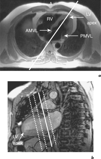
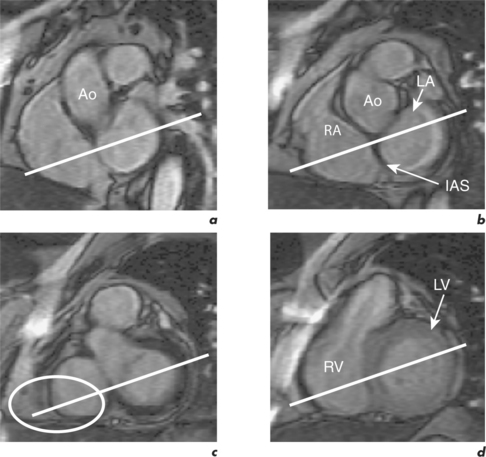
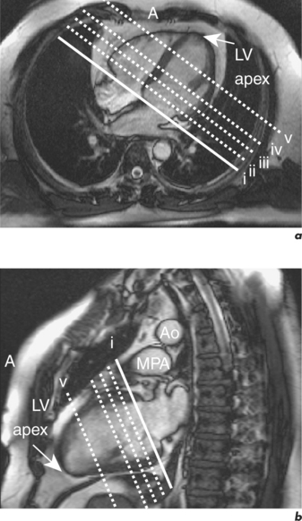
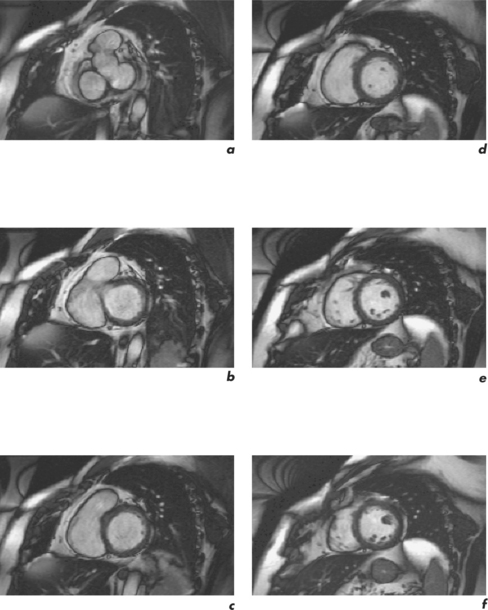
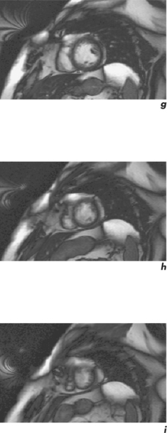
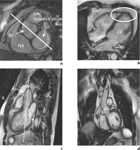
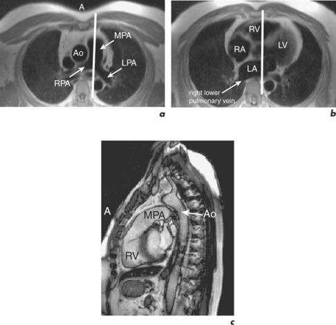
Table 1.1 A standard CMR protocol which typically takes 30 minutes to perform
| Pre-contrast |
| Five-slice SSFP pilot |
| Free breathing, low-resolution transaxial FSE |
| Breath-hold, low-resolution coronal (+ sagittal) FSE |
| Two-chamber pilot |
| Four short-axial pilots |
| Four-chamber and two-chamber cines |
| LVOT and RVOT cines |
| Ventricular short-axis stack cines |
| Post-contrast |
| Early gadolinium enhancement (1–5 minutes) |
| (a) Rpt four-chamber |
| (b) Rpt two-chamber |
| (c) Rpt LVOT |
| Late gadolinium enhancement (5–15 minutes) |
| (a) Rpt four-chamber |
| (b) Rpt two-chamber |
| (c) Rpt ventricular short-axis stack |
Protocols for cardiac imaging involve four stages:
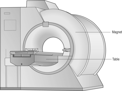
The initial pilot images are performed in a breath-hold and are used to optimize subject placement within the magnetic field using the table-positioning tool—the centre of the heart should be at the centre of the field. The pilot scan also enables the user to check that the correct coils are activated and other system requirements are satisfactory. Subsequent low-resolution anatomical coverage using FSE acquires one image per cardiac cycle. This allows a ‘quick-look’ for cardiac and extracardiac pathology at the start of the study and resulting images must be reviewed prior to further acquisitions. A series of transaxial FSE images usually consists of 35–40 slices, performed in free breathing over 1–2 minutes. A 12- to 15-slice series of coronal and sagittal FSE images encompass the heart and can be performed in a breath-hold. Breath-hold images do enable more accurate positioning of subsequent slices, but respiratory variations are small within the transaxial plane. Acquisition of the standard planes has been detailed in Figures 1.4–1.9. Additional targeted planes and sequences are chosen depending on the referral request, and presence and type of other pathology.
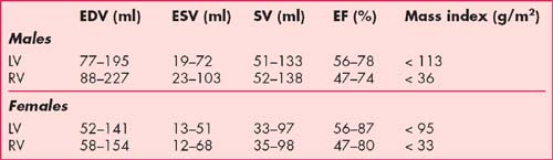
Normal ranges
The normal ranges for end-diastolic volumes (EDV), end-systolic volumes (ESV), stroke volumes (SV), ejection fraction (EF) and myocardial mass indexes in males and females are presented in Table 1.2. These values are calculated using semi-automated software analysis tools applied to the ventricular short-axis stack of GE cines. Calculation of LV parameters is performed in approximately 5 minutes while RV parameters take longer because of the more complex anatomy. Quantification of LV parameters is mandatory for CMR reporting and RV parameters are calculated as required, for example in patients with congenital heart disease, arrhythmogenic right ventricular cardiomyopathy (ARVC), dilated cardiomyopathy (DCM) and cases of valvular regurgitation. Normal ranges are age and body surface area dependent and normatized values are also available.
Other important cardiovascular normal ranges, including dimensions for the aorta and pulmonary vessels, are currently based on echocardiographic data, since CMR specific values are yet to be published (Table 1.3).
Table 1.3 Normal ranges for cardiovascular structures by echocardiography
| Cardiovascular structure | Range (cm) |
|---|---|
| Aorta dimensions (end-diastole) | |
| Aortic annulus | 1.4–2.6 |
| Sinus of Valsalva | 2.1–3.5 |
| Sinotubular junction | 1.7–3.4 |
| Ascending aorta (at MPA bifurcation) | 2.1–3.4 |
| Aortic arch | 2.0–3.6 |
| Descending thoracic aorta (at MPA bifurcation) | 1.4–3.0 |
| Distal descending thoracic aorta | 1.3–2.8 |
| LVOT (diastole) | 1.4–2.6 |
| RVOT (diastole) | 1.8–3.4 |
| PA dimensions (end-diastole) | |
| Pulmonary annulus | 1.0–2.2 |
| MPA | 0.9–2.9 |
| RPA | 0.7–1.7 |
| LPA | 0.6–1.4 |
| Venous dimensions | |
| Pulmonary | 0.7–1.6 |
| Inferior vena cava | 1.2–2.3 |
| Superior vena cava | 0.8–2.0 |
| Hepatic | 0.5–1.1 |
Indications
The European Society of Cardiology published guidelines in November 2004 on the clinical indications for CMR (Tables 1.4–1.8) with the usefulness of this imaging technique in specific diseases classified as follows:
| Indication | Class | |
|---|---|---|
| 1. | Assessment of global ventricular (left and right) function and mass | I |
| 2. | Detection of CAD | |
| Regional LV function at rest and during dobutamine stress | II | |
| Assessment of myocardial perfusion | II | |
| Coronary MRA (CAD) | III | |
| Coronary MRA (anomalies) | I | |
| Coronary MRA of bypass graft patency | II | |
| CMR flow measurements in the coronary arteries | Inv | |
| Arterial wall imaging | Inv | |
| 3. | Acute and chronic myocardial infarction (MI) | |
| Detection and assessment | I | |
| Myocardial viability | I | |
| Ventricular septal defect | III | |
| Mitral regurgitation (acute MI) | III | |
| Ventricular thrombus | II | |
| Acute coronary syndromes | Inv | |
Table 1.5 Indications for CMR in patients with pericardial disease, cardiac tumours, cardiomyopathies and cardiac transplants
| Indication | Class | |
|---|---|---|
| 1. | Pericardial effusion | III |
| 2. | Constrictive pericarditis | II |
| 3. | Detection and characterization of cardiac and pericardiac tumours | I |
| 4. | Ventricular thrombus | II |
| 5. | Hypertrophic cardiomyopathy | |
| Apical | I | |
| Non-apical | II | |
| 6. | DCM | Inv |
| Differentiation from dysfunction related to coronary artery disease | I | |
| 7. | ARVC | I |
| 8. | Restrictive cardiomyopathy | II |
| 9. | Siderotic cardiomyopathy (in particular thalassaemia) | I |
| 10. | Non-compaction | II |
| 11. | Post-cardiac transplantation rejection | Inv |
Table 1.6 Indications for CMR in patients with valvular heart disease
| Indication | Class | |
|---|---|---|
| 1. | Valve morphology | |
| Bicuspic AV | II | |
| Other valves | III | |
| Vegetations | Inv | |
| 2. | Cardiac chamber anatomy and function | I |
| 3. | Quantification of regurgitation | I |
| 4. | Quantification of stenosis | III |
| 5. | Detection of paravalvular abscess | Inv |
| 6. | Assessment of prosthetic valves | Inv |
Table 1.7 Indications for CMR in congenital heart disease
| Indication | Class | |
|---|---|---|
| General indications | ||
| 1. | Initial evaluation and follow-up of adult congenital heart disease | I |
| Specific indications | ||
| 1. | Assessment of shunt size (Qp/Qs) | I |
| 2. | Anomalies of the viscero-atrial situs | I |
| Isolated situs anomalies | II | |
| Situs anomalies with complex congenital heart disease | I | |
| 3. | Anomalies of the atria and venous return | |
| Atrial septal defect (secundum and primum) | II | |
| Anomalous pulmonary venous return, especially in complex anomalies and cor triatriatum | I | |
| Anomalous systemic venous return | I | |
| Systemic or pulmonary venous obstruction following intra-atrial baffle repair or correction of anomalous pulmonary venous return | I | |
| 4. | Anomalies of the atrioventricular valves | |
| Anatomic anomalies of the mitral and tricuspid valves | II | |
| Functional valvular anomalies | II | |
| Ebstein’s anomaly | II | |
| Atrioventricular septal defect | II | |
| 5. | Anomalies of the ventricles | |
| Isolated ventricular septal defect (VSD) | III | |
| VSD associated with complex anomalies | I | |
| Ventricular aneurysms and diverticula | II | |
| Supracristal VSD | I | |
| Evaluation of right and left ventricular volumes, mass and function | I | |
| 6. | Anomalies of the semilunar valves | |
| Isolated valvular pulmonary stenosis and valvular dysplasia | III | |
| Supravalvular pulmonary stenosis | II | |
| Pulmonary regurgitation | I | |
| Isolated valvular AS | III | |
| Subaortic stenosis | III | |
| Supravalvular AS | I | |
| 7. | Anomalies of the arteries | |
| Malpositions of the great arteries | II | |
| Post-operative follow-up of shunts | I | |
| Aortic (sinus of Valsalva) aneurysm | I | |
| Aortic coarctation | I | |
| Vascular rings | I | |
| Patent ductus arteriosus | III | |
| Aortopulmonary window | I | |
| Coronary artery anomalies in infants | Inv | |
| Anomalous origin of coronary arteries in adults and children | I | |
| Pulmonary atresia | I | |
| Central pulmonary stenosis | I | |
| Peripheral pulmonary stenosis | Inv | |
| Systemic to pulmonary collaterals | I | |
Table 1.8 Indications for CMR in acquired diseases of the vessels
| Indication | Class | |
|---|---|---|
| 1. | Diagnosis and follow-up of thoracic aortic aneurysm including Marfan disease | I |
| 2. | Diagnosis and planning of stent treatment for abdominal aortic aneurysm | II |
| 3. | Aortic dissection | |
| Diagnosis of acute aortic dissection | II | |
| Diagnosis and follow-up of chronic aortic dissection | I | |
| 4. | Diagnosis of aortic intramural haemorrhage | I |
| 5. | Diagnosis of penetrating ulcers of the aorta | I |
| 6. | PA anatomy and flow | I |
| 7. | Pulmonary emboli | |
| Diagnosis of central pulmonary emboli | III | |
| Diagnosis of peripheral pulmonary emboli | Inv | |
| 8. | Assessment of thoracic, abdominal and pelvic veins | I |
| 9. | Assessment of leg veins | II |
| 10. | Assessment of renal arteries | I |
| 11. | Assessment of mesenteric arteries | II |
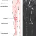
| 12. | Assessment of iliac, femoral and lower leg arteries | I |
| 13. | Assessment of thoracic great vessel origins | I |
| 14. | Assessment of cervical carotid arteries | I |
| 15. | Assessment of atherosclerotic plaque in carotid artery/aorta | III |
| 16. | Assessment of pulmonary veins | I |
| 17. | Endothelial function | Inv |
Tables 1.4, 1.5, 1.6, 1.7 and 1.8 used with kind permission of European Society of Cardiology from Pennell et al Clinical Indications for Cardiovascular Magnetic Resonance (CMR): Consensus Panel Report, European Heart Journal, 2004, 25 (21), 1940–1965.
Contraindications and issues of safety
The environment in which CMR is performed must be constantly protected from the inadvertent introduction of ferromagnetic metallic objects and electronic equipment near the powerful magnetic field, with safety failures possibly leading to injury and rare cases of mortality. Potential subjects fill out a checklist as shown in Figure 1.10, which is then reviewed by trained personnel prior to placement within the magnet. Regular cardiorespiratory arrest scenario training in the safe and speedy removal of subjects undergoing CMR to nearby, designated resuscitation areas are advocated for clinical and allied MRI staff.