Chapter 2 Practical Considerations
Ultrasonographic instrument design
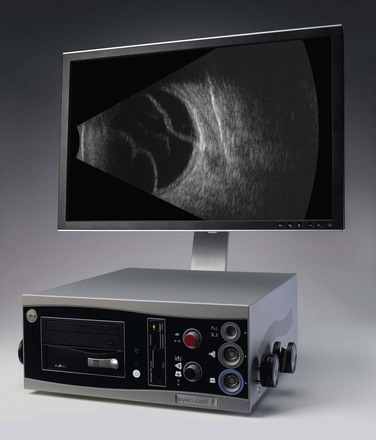
All ultrasonographic devices have four essential components: a pulse source, a transducer, a receiver, and a display screen (Figure 2.1). The ultrasound pulser produces multiple short electric pulses. The voltage pulses are sent to the transducer where a piezoelectric crystal converts electrical energy into mechanical vibrations. The vibrations generate longitudinal ultrasound waves that travel through tissues in contact with the transducer/probe. At each change in tissue density (acoustic interface) echoes are reflected back towards the transducer. Between pulses of several microseconds, the returning echoes hit the transducer and the piezoelectric crystal turns the mechanical energy into electrical energy. The resulting electrical signals are detected by the receiver, processed and displayed in real time (Chapter 1).
Axial resolution
The axial resolution, or minimum distance between two echo sources, is directly related to frequency, piezoelectric crystal shape and the damping material attached to the crystal.1–3 The higher the frequency of the generated sound waves, the higher the axial resolution. For example a 10 MHz contact B-scan probe used to examine the posterior segment has an axial resolution of approximately 100 µm, while a 50 MHz ultrasound biomicroscopy probe used to examine the anterior segment has an axial resolution of approximately 37 µm (Figure 2.2) (Chapter 4). Frequencies utilized in ophthalmic ultrasonography are higher than those used in other fields of diagnostic ultrasonography, resulting in enhanced detection of small irregularities of the eye and orbit that are undetectable in structures more internally located (Chapter 1).4
Amplification curves
The echoes returning to the ultrasonographic instrument between pulses of ultrasound propagation have weak frequency signals. The receiver in the instrument must then process the signals using a combination of amplification, compression, compensation, demodulation and rejection.4 The most important of these complex-processing tools is amplification. Amplification of the sound waves can be linear, logarithmic and S-shaped. The type of amplification curve directly affects the dynamic range. The dynamic range is defined as the range of echo intensities that can be displayed and is labeled in units of decibels (dB). Linear curve amplifiers have a small dynamic range and logarithmic amplifiers have a large dynamic range. However, linear amplifiers are sensitive to minor differences in the density of echo sources while logarithmic amplifiers are not. The most common type of amplification curve used in ophthalmic ultrasonography is S-shaped as it offers the sensitivity of linear amplification and the dynamic range of logarithmic amplification. The S-shaped curve is used in standardized echography to enhance ophthalmic tissue differentiation without losing range of detection (Chapter 1).5–7
Gain
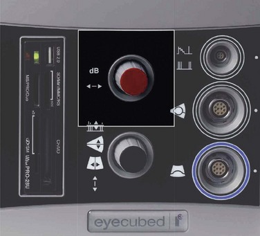
Ultrasonography machines also allow the user to manually adjust the amplification of echo signals displayed on the screen by adjusting the gain (Figure 2.3). Gain is a measurement of intensity labeled in decibels (dB). Adjusting the gain does not change the frequencies or pulse length of the emitted ultrasound waves. It only changes the intensity of the echo pattern displayed. Gain settings vary slightly based on the manufacturer, but in general gain settings range from 30 to 100 dB. At a low gain, only strong echo sources are visible. Lowering the gain has the effect of decreasing the depth of sound penetration and narrowing the sound beam resulting in increased resolution. The choroid, sclera and orbital structures are usually best examined at a low gain (Chapter 3). At a high gain, weaker echo sources are detected, but resolution is effectively lost. Vitreous opacities and thin vitreous membranes are best examined at high gain (Chapter 10). Most machines also have an internal time gain compensation control (TGC). It will amplify weaker echoes resulting from deeper tissues slightly more than those echoes from more superficial tissues, thus equalizing the echo strength from similar tissues located at varied distances from the transducer/probe.
Ophthalmic ultrasonography modules
In addition to a pulse source, transducer, receiver and display screen, most current ophthalmic ultrasonographic devices are optimized for use with multiple probes. Typical instruments are able to accommodate a 10–12 MHz biometric A-scan probe, an 8 MHz standardized A-scan probe, and a 10 MHz contact B-scan probe. High-resolution ophthalmic ultrasound or ultrasound biomicroscopy (UBM) probes ranging from 20 to 80 MHz are additionally available on many modules (Chapter 4).
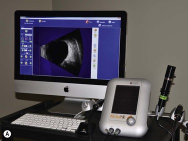
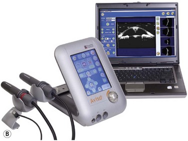
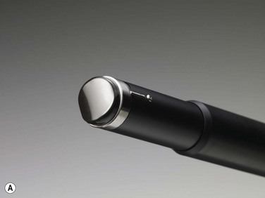
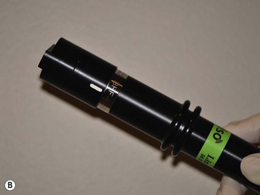
Both contact B-scan probes and UBM probes produce two-dimensional images using echo displays of the horizontal and vertical axis and thus, both have transducers that rapidly oscillate back and forth. However, the probes have very different appearances. The 10 MHz transducer is submerged in liquid and covered to create a smooth probe tip (Figure 2.4A). UBM transducers are uncovered requiring extreme care while performing the examination (Figure 2.4B). A water bath or cover is necessary to provide the stand off distance to avoid distortion of structures close to the transducer. The water bath also avoids sound attenuation due to a covering membrane limiting depth penetration and resolution (Chapter 4).8,9
Future improvements
The field of ophthalmic ultrasonography is undergoing technological advances with the use of nanotechnology applications in creating novel transducer materials capable of generating frequencies higher than 100 MHz.10 Ophthalmic applications of Doppler ultrasonography and contrast enhanced ultrasonography are currently under investigation (Chapter 5). Other enhancements such as 3D ultrasonography, superharmonic ultrasonography, photoacoustic imaging, and robotic applications are discussed elsewhere (Chapter 19).
1 Lizzi FL, Feleeppa EJ. Practical physics and electronics of ultrasound. Int Ophthalmol Clin. 1979;19(4):35-66.
2 Fisher YL. Contact B-scan ultrasonography: a practical approach. Int Ophthalmol Clin. 1979;19(4):103-126.
3 Bryne S, Green R. Ultrasound of the Eye and Orbit, 2nd ed. St. Louis: Mosby; 2002.
4 Lizzi FL, Coleman DJ. History of ophthalmic ultrasound. J Ultrasound Med. 2004;23(10):1255-1266.
5 Ossoinig KC. Quantitative echography – the basis of tissue differentiation. J Clin Ultrasound. 1974;2(1):33-46.
6 Ossoinig KC. Standardized echography: basic principles, clinical applications, and results. Int Ophthalmol Clin. 1979;19(4):127-210.
7 Ossoinig KC, Byrne SF, Weyer NJ. Part II: Performance of standardized echography by the technician. Int Ophthalmol Clin. 1979;19(4):283-286.
8 Pavlin CJ, Harasiewicz K, Sherar MD, et al. Clinical use of ultrasound biomicroscopy. Ophthalmology. 1991;98(3):287-295.
9 Pavlin CJ, Foster FS. Ultrasound biomicroscopy. High-frequency ultrasound imaging of the eye at microscopic resolution. Radiol Clin North Am. 1998;36(6):1047-1058.
10 Foster FS, Pavlin CJ, Harasiewicz KA, et al. Advances in ultrasound biomicroscopy. Ultrasound Med Biol. 2000;26(1):1-27.