FUNDAMENTALS OF X-RAY PHYSICS

In the diagnostic x-ray energy range between 20 keV and 140 keV, there are three types of interactions between x-ray photons and the patient: photoelectric effect, Compton scatter, and coherent scatter.^1–3 In photoelectric interaction, the incident x-ray photon energy is greater than the binding energy of a deep shell electron. By giving up its entire energy in liberating the electron, the original x-ray photon no longer exists. When the hole created at the deep shell is filled by an outer shell electron, a characteristic radiation is generated. Because the probability of such interaction is proportional to the cube of the atomic number of the matter, tissues with small differences in atomic numbers result in a greater difference in the x-ray photon absorption and lead to greater contrast between different tissues.

In Compton scatter interaction, the energy of the incident x-ray photon is considerably higher than the binding energy of the electron, and the incident x-ray photon is deflected or scattered with partial loss of its initial energy while freeing up the electron from the atom. The scattered photon may be deflected at any angle ranging from 0 to 180 degrees and consequently provides little information about the location of interaction and the original photon path. The scattered photon may undergo additional collisions before exiting the patient. This type of interaction is the most important interaction mechanism in tissue-like materials.

The third and less important type of interaction is the coherent scattering or Rayleigh scattering. Little energy is lost in such interaction. In medical imaging, all three types of interactions are combined in the measurement, and only the composite effect is observed. Interaction of x-ray photons with matter is governed by Beer’s law, which can be described by the following equation for a monoenergetic x-ray beam:

where I₀ is the intensity of the x-ray beam impinging on a uniform material of thickness Δx, I is the x-ray intensity after passing through the material, and µ is the linear attenuation coefficient of the material; µ changes with the input x-ray energy and varies for different materials. Figure 79-1 shows, on a logarithmic scale, µ as a function of energy for soft tissue (red), cortical bone (green), and iodine (blue). It is clear from the figure that significant difference exists between the attenuation coefficients for the three materials, and iodine is more attenuating to the x-ray photons than the bone, which in turn is more attenuating than the soft tissue. As a result, when iodine-based contrast material is injected intravenously into the patient and imaged under x-ray examination, blood vessels generate stronger attenuating signals and therefore become more visible over the diagnostic x-ray energy range.

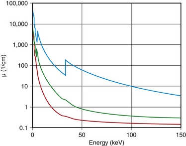
FIGURE 79-1 Linear attenuation coefficients as a function of energy: red, soft tissue; green, bone; blue, iodine.

The x-ray photons produced by the x-ray tube on all clinical x-ray devices today have a wide energy spectrum. For example, when 120 kVp is prescribed on an x-ray CT scanner, x-ray energies ranging from 20 keV to 120 keV are emitted. Because the amount of attenuation to these x-ray photons varies significantly, even for a single material as demonstrated in Figure 79-1, the measured attenuation of an object is consequently the averaged effects of different energy x-ray photons weighted by their spectrum.

IMPORTANT PERFORMANCE PARAMETERS OF X-RAY COMPUTED TOMOGRAPHY

There are many parameters that define the performance of a CT scanner.^1,4–6 During the system design, conscious decisions have to be made to trade off some performance parameters against others to optimize the overall performance for a particular application. In this section, a few important performance parameters of the CT system are discussed, and it should be understood that this is by no means a complete list.

Spatial resolution defines the ability of a CT scanner to resolve closely spaced high-contrast objects and is often specified in terms of line pairs per centimeter (lp/cm). A pattern of 1 lp/cm is formed by a pair of high- and low-intensity bars, each 5 mm in width, as shown in Figure 79-2A; a pattern of 4 lp/cm contains four such high- and low-intensity bars within each centimeter space, as depicted in Figure 79-2B. It is clear from the figure that as the width of the bars is reduced and the bars are closely packed together, it becomes increasingly difficult for a CT system to resolve or to identify the bars individually. To measure the spatial resolution of a CT system, standard bar phantoms are scanned and reconstructed. An example of such a phantom (Catphan) is shown in Figure 79-3. In this phantom, bar patterns of different frequencies are positioned at a fixed radius from the phantom center, and system response to these frequencies can be evaluated from a single scan.

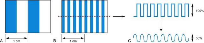
FIGURE 79-2 Illustration of CT resolution testing pattern: A, 1 lp/cm; B, 4 lp/cm; C, profiles of the object and reconstructed image.

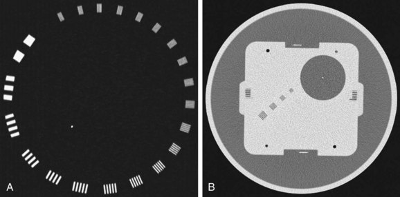
FIGURE 79-3 Reconstructed images of resolution phantoms. A, Catphan. B, GE Performance phantom.

(B courtesy of GE Healthcare Technologies, Waukesha, Wisc.)

To quantitatively describe the spatial resolution performance, modulation transfer function (MTF) is typically employed. If we plot the profile of the original 4 lp/cm bar pattern object, we obtain a set of rectangular functions as shown by the upper portion of Figure 79-3C. In a similar fashion, we can plot the profile of the reconstructed image of the same bar pattern and obtain a smoothed version of the original rectangular pattern shown by the lower portion of Figure 79-2C. Because of the limited frequency response of the system, both the sharpness and the peak-to-valley magnitude of the reconstructed bar pattern are reduced compared with the original. In the example shown, the magnitude of the reconstructed object is only 50% of the original. Therefore, the MTF value at 4 lp/cm for this system is 0.5. By plotting the peak-to-valley magnitude over different frequencies, a complete MTF curve is obtained. The MTF accurately describes a system’s frequency response and is a good indicator of the system’s ability to resolve small objects. Alternatively, MTF curves can be obtained from the reconstructed phantom image of a thin wire, based on the fact that MTF is the magnitude of the Fourier transform of the point-spread function. Figure 79-3B shows a reconstructed image of a GE Performance phantom, and the wire section of the image is extracted to generate the MTF curve.

The most commonly quoted spatial resolution specifications are the 50% MTF, 10% MTF, and 0% MTF, which represent the frequencies at which the peak-to-valley magnitude of the CT system drops to 50%, 10%, and 0% of the scanned bar pattern. There are many factors that have an impact on the MTF, such as x-ray focal spot size, detector size, sampling frequency, system geometry, and reconstruction algorithm.

The importance of spatial resolution can be easily understood because it is an indicator of how well a small structure can be visualized. For example, Figure 79-4 depicts a volume rendered image of a CT angiography scan collected on a multislice CT scanner. High spatial resolution enables the clear visualization of small vascular structures. Another example is depicted in Figure 79-5 of two volume rendered images of a stent. Clear visualization of the stent allows the evaluation and assessment of its integrity or potential of restenosis in many clinical applications. Figure 79-5A was obtained on a multislice CT scanner; Figure 79-5B was obtained on a high-definition scanner. Because of the increased spatial resolution offered by the high-definition scanner, the stent structure is better visualized.

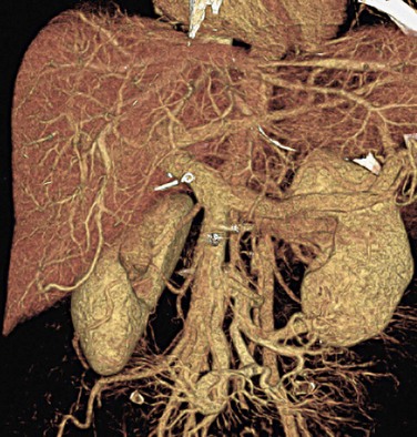
FIGURE 79-4 CT angiography study of a patient performed on a multislice CT scanner.

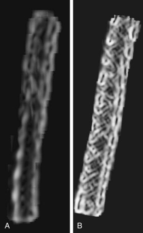
FIGURE 79-5 Volume rendered images of a 3-mm stent. A, The multislice CT image. B, High-definition image.

(Courtesy of GE Healthcare Technologies, Waukesha, Wisc.)

Another important performance parameter is the CT number uniformity and accuracy. CT number is defined by the following equation:

where µ is the linear attenuation coefficient of the object of interest and µ_w is the linear attenuation coefficient of water; the quantity is measured in Hounsfield units, honoring the inventor of the x-ray CT scan. On the basis of this definition, water automatically has a value of zero and air has a value of −1000. To ensure the CT number accuracy, water phantoms are often scanned, and the average CT number inside the water phantom is measured to ensure that it is within the tolerance limit of a few Hounsfield units. The selection of water phantoms for quality control is not accidental because the attenuation characteristics of human soft tissues are similar to those of water. Figure 79-6 depicts the reconstructed image of a 20-cm water phantom. For typical tests, several regions of interest are selected across the entire phantom to ensure that the CT number accuracy is maintained in the entire reconstruction field of view.

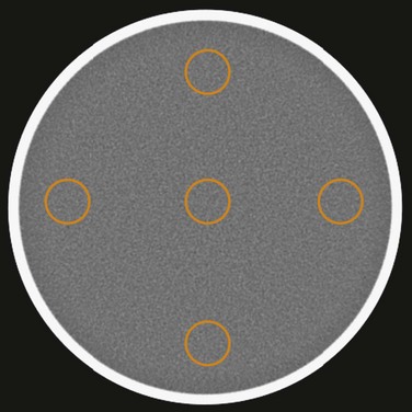
FIGURE 79-6 Reconstructed image of a 20-cm water phantom.

The CT number accuracy of a CT scanner can be affected by many factors, such as beam hardening, scatter, long-term stability of components, and other calibration issues. Therefore, periodic quality assurance testing is necessary to ensure that a CT scanner is performing within its designed specification. Recent research and development activities of dual-energy CT place an even higher importance on CT number accuracy because good material decomposition relies on the accuracy and reproducibility of the reconstructed CT numbers of different materials.

One of the more complex performance parameters is perhaps the low contrast detectability (LCD). LCD indicates a scanner’s ability to identify small objects whose CT number difference to their background is small, and its performance depends not only on the size and contrast of the low-contrast objects to their background but also on the noise level present in the image. Because noise in the image is closely linked to the noise in the projection data, LCD needs to be specified with the specific phantom used in the test and the dose level in the scan. For example, the LCD specification generated with a Catphan of 3 mm, 0.3%, at 18 mGy and 5-mm slice thickness indicates that when the phantom is scanned with a dose level of 18 mGy and reconstructed at 5-mm slice thickness, 3-mm objects with 3 HU difference to their background can be visualized. For illustration, Figure 79-7A shows a reconstructed LCD section of a Catphan. Cylindrical objects of various sizes and contrast levels to the background are contained in the phantom of uniform background. Historically, the LCD specification was generated with human observers. Each observer was asked to identify the smallest cylinder with the lowest contrast in a set of reconstructed images. By incorporation of results generated on multiple images and with multiple observers, the LCD specification was produced. It is clear that such a method is highly subjective, and large variation among observers is expected. To overcome such shortcoming, several image processing–based methodologies were proposed. Given the limited scope of this chapter, any details are not discussed here.

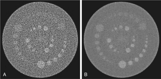
FIGURE 79-7 Reconstructed images of a Catphan LCD section. A, Conventional filtered back-projection reconstruction. B, Advanced statistical reconstruction.

Because image noise plays an important role in LCD, it is important to understand the impact of the reconstruction algorithm on LCD. For illustration, Figure 79-7 depicts the same LCD scan data reconstructed with two different reconstruction algorithms. The image depicted in Figure 79-7A was reconstructed with a filtered back-projection algorithm, which is a class of algorithm used by all vendors on the commercially available clinical scanners. The image depicted in Figure 79-7B, on the other hand, was reconstructed with an advanced statistical reconstruction that accurately models the statistics of the CT system. It is clear that better visualization of the LCD objects is achieved by the advanced statistical reconstruction. The 0.3% disks (shown in the outer ring between the 12- and 2-o’clock positions) that cannot be resolved in Figure 79-7A are now visible in Figure 79-7B. A similar result is also observed in a clinical study performed on a multislice CT scanner, as shown in Figure 79-8A and B. Note that by suppressing the noise in the images generated by filtered back-projection, density variations in the low-contrast tissues can be better visualized in Figure 79-8B.

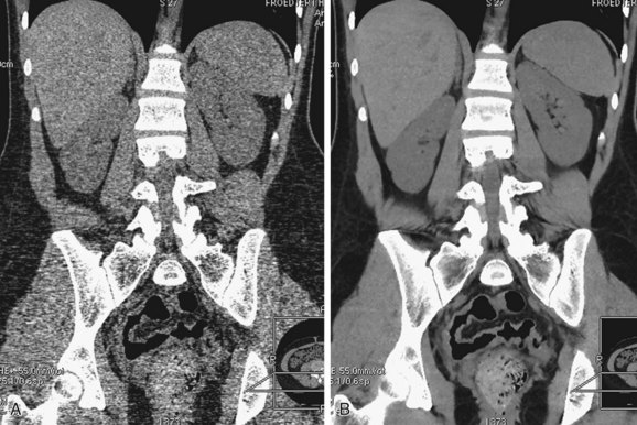
FIGURE 79-8 Coronal images of a patient’s scan on a multislice CT scanner. A, Conventional filtered back-projection reconstruction. B, Advanced statistical reconstruction.

There are other performance parameters important to the specification of a CT scanner, such as temporal resolution, image artifacts, noise uniformity, spatial resolution uniformity, and dose efficiency. Interested readers can find relevant material in reference 1.

STEP-AND-SHOOT VERSUS HELICAL

Helical or spiral CT (HCT) was introduced in the early 1990s to overcome the lengthy delay in the traditional step-and-shoot mode of data acquisition.^7–10 Before the introduction of HCT, the patient and the table remained stationary during the data acquisition. Once the data collection is completed, the table is indexed to the next location for scanning. The table indexing time is typically on the order of a second. When the gantry rotation speed is slow, the amount of time spent on table translation is relatively small and constitutes a small fraction of the total study time. As the gantry speed increases, the table translation time becomes a significant portion of the overall scan time. Considering that the patient is holding his or her breath during CT scans to reduce motion-induced artifacts, a significant portion of the patient breath-hold time is wasted on indexing the patient because no data acquisition takes place during the patient indexing.

In HCT, the patient’s table is translated at a constant speed while continuous data acquisition takes place. Relative to a fixed location on the patient, the x-ray source trajectory forms a helix (shown in Fig. 79-9), and the name of HCT is a reflection of such trajectory. In the early days of HCT development, there were lively debates on the naming convention: helical versus spiral. These debates ended without a clear winner, and both names are used interchangeably today.

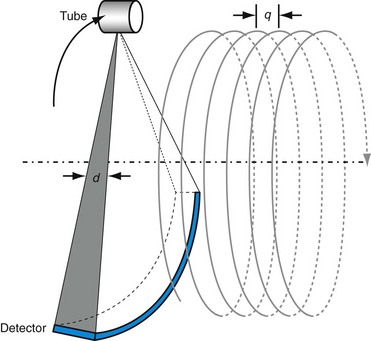
FIGURE 79-9 Illustration of helical data acquisition.

To characterize the nature of the helical trajectory, helical pitch is typically used. Helical pitch, h, is defined as the ratio of the table traveling distance in one gantry rotation, q, over the x-ray beam collimation width at the isocenter, d:

A higher h value indicates a faster table translation, assuming the gantry rotation speed is kept constant. An added advantage of the HCT mode of acquisition is the uniform sampling pattern along the patient’s long axis. Note that in the step-and-shoot mode of data acquisition, the patient is scanned at discrete locations. For example, if a 2.5-mm source collimation is used for data acquisition, the table is typically indexed every 2.5 mm to acquire a consecutive set of slices. In HCT mode, however, the table moves in a continuous fashion, and the data are collected uniformly along the patient’s long axis, z. Because the data acquisition is uniform along z, images can be reconstructed at arbitrary locations and spacing. If we use the same 2.5-mm source collimation example, images can be reconstructed at every 1.25 mm or finer to satisfy the Nyquist sampling criteria and to enable improved image quality in reformatted or volume rendered images. For illustration, Figure 79-10A shows a coronal image of a patient’s scan reconstructed with 2.5-mm slice thickness at 2.5-mm spacing. Close inspection of the boundaries of the air pockets and contrast-enhanced organs shows discontinuities or stair-stepping artifacts, a clear indication of undersampling along the z-axis. For helical reconstruction, the images are reconstructed with the same slice thickness (2.5 mm) but at 1.0-mm spacing. Stair-stepping artifacts are completely eliminated in the coronal image as shown in Figure 79-10B. These advantages come at the price of increased complexity in reconstruction.

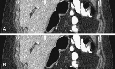
FIGURE 79-10 Coronal images of a clinical study. A, A 2.5-mm slice thickness without overlap. B, A 2.5-mm slice at 1.0-mm spacing.

Less than a decade ago, the majority of the commercially available CT scanners were built with single-row detectors, in which the coverage along the patient’s long axis is linked directly to the pre-patient collimation and the slice thickness. To scan a large volume in a short time for CT angiography applications (to keep up with the contrast bolus), higher helical pitch (h) was often used. For a single-slice scanner, a higher helical pitch often leads to an increased level of helical artifacts and degraded slice profiles. One often must trade off the coverage speed with the image quality. For illustration, Figure 79-11 shows the reconstructed images of a helical body phantom. The oval high-density objects are ellipsoids placed at an angle with respect to the patient’s long axis to simulate ribs. The air pocket at the center is shaped as an ellipsoid. It is clear from the figure that as the helical pitch increases, the distortion and shading artifacts around ribs and air pocket increase. The monotonic behavior of artifacts versus helical pitch is mainly a single-slice scanner behavior. The relationship between artifacts and helical pitch is more complex for the case of a multislice scanner.

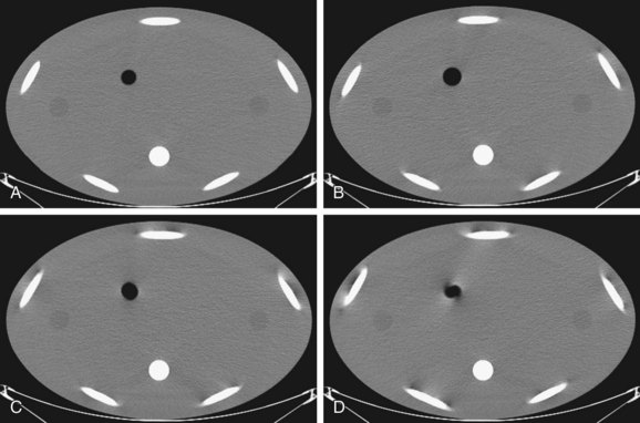
FIGURE 79-11 Helical artifacts increase with an increase in helical pitch for a single slice: A, h = 0; B, h = 1; C, h = 1.5; D, h = 2.0.

There are other considerations in the selection of the helical pitch as well. One of the considerations is the noise level in the reconstructed images. As a general rule of thumb, the number of projections used to reconstruct an image is roughly inversely proportional to the helical pitch. For example, the number of views used in a 0.5 : 1 pitch scan is roughly twice as many as the number of views used in the 1 : 1 pitch. If other scanning parameters are kept constant, the 0.5 pitch image will be generated with nearly twice as much photon flux as the pitch 1 case; thus, the noise in the image should be scaled down by roughly . This offers additional flexibility in scanning of large patients when the maximum x-ray tube power is limited.

MULTISLICE COMPUTED TOMOGRAPHY

Although the very first CT scanner built more than three decades ago was a multislice CT scanner (dual slice), many people consider the commercial introduction of the four-slice scanner in the late 1990s the turning point of the multislice revolution, a reflection of its clinical impact, not a simple specification or slice count.^11–14 As the name implies, a multislice CT scanner divides each single-row detector cell into multiple detector cells along the gantry rotation axis (z-axis), as shown in Figure 79-12.

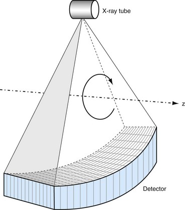
FIGURE 79-12 Illustration of multislice CT configuration.

The advantage of the multislice CT scanner is its large detector coverage along the patient’s long axis without trading off the spatial resolution in z. In a single-slice scanner, the z-coverage and the slice thickness are both controlled by the pre-patient collimator. If a 10-mm z-coverage is desired, the slice thickness of the detector is also 10 mm. Therefore, there is a one-to-one relationship between the coverage and z-resolution. For a multislice scanner, the slice thickness is no longer determined by the pre-patient collimation; it is determined by the size of the finely divided detector cells (if we ignore focal spot size and other factors). A larger coverage in z requires a larger number of detector rows.

There are two different types of detector designs used in the multislice CT scanner: matrix detector and adaptive detector (Fig. 79-13). In the matrix detector configuration, all detector rows are diced into identical sizes, and acquisition slice thickness is solely defined by the detector cell size. Different slice thickness can be obtained by combining several detector rows before or during the reconstruction process. In the adaptive detector scheme, the sizes of detector rows change symmetrically with respect to the detector center, and acquisition slice thickness is defined by the combination of detector cell aperture and pre-patient collimation. Similar to the matrix detector configuration, different slice thickness can be achieved by combining multiple detector rows. There are pros and cons with each approach, and given the limited scope of this chapter, detailed discussion is omitted here.

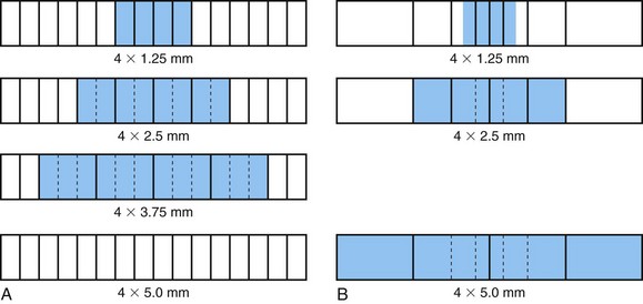
FIGURE 79-13 Illustration of different detector configurations. A, Matrix configuration. B, Adaptive configuration.

If the introduction of helical CT marks the era of single-organ coverage in a single breath-hold, the realization of the multislice CT marks the era of isotropic spatial resolution anywhere at any time. With the introduction of the 64-slice scanners, the time it takes to scan an anatomy in most cases is no longer limited by the data acquisition speed of the scanner. In fact, in many clinical practices, the scan speed is purposely throttled back to avoid over-running the contrast agent.

There are many technical challenges facing multislice CT development as the number of slices increases significantly beyond 64-slice configuration. These challenges include the cone-beam artifacts for step-and-shoot mode scans, longitudinal truncation issues, over-beaming issues, increased scatter, degraded heel effect of the x-ray tube, compromised dose efficiency, and reduced effectiveness of the x-ray tube current modulation. Some of the challenges, such as over-beaming, can be addressed by modification of existing CT designs. Other challenges, such as cone-beam artifacts for step-and-shoot mode acquisition, remain difficult, and significant research efforts are continuing to minimize their clinical impact.

KEY POINTS

Important parameters that define the performance of a CT scanner include spatial resolution, CT number uniformity and accuracy, and low contrast detectability.

Temporal resolution, image artifacts, noise uniformity, spatial resolution uniformity, and dose efficiency are other parameters of performance.

Helical CT uses continuous table translation during scanning, which is faster than step-and-shoot scanning and avoids misregistration artifact.

Multislice CT allow fast scanning of a large volume, which is ideal for vascular imaging.